FACULDADE DE CIˆ
ENCIAS
DEPARTAMENTO DE F´
ISICA
Development of motion
compensated 3D T2 mapping for
cardiac imaging
Jo˜
ao Lu´ıs Silva Canaveira Tourais
Tese orientada por:
Prof. Dr. Ren´e Botnar, Division of Imaging Sciences & Biomedical Engineering, King’s College London, United Kingdom
Dr. Rita Nunes, Instituto de Biof´ısica e Engenharia Biom´edica, Departamento de F´ısica da Faculdade de Ciˆencias da Universidade de Lisboa, Portugal
MESTRADO INTEGRADO EM ENGENHARIA BIOM´EDICA E BIOF´ISICA Perfil de Engenharia Cl´ınica e Instrumenta¸c˜ao M´edica
DISSERTAC¸ ˜AO
A Ressonˆancia Magn´etica Card´ıaca (RMC) tem vindo a crescer tendo-se tornado numa excelente t´ecnica de avalia¸c˜ao de doen¸cas card´ıacas, uma vez que produz ima-gens do cora¸c˜ao de alta qualidade e de forma n˜ao ionizante. O edema do mioc´ardio ´e uma patologia em que ocorre aumento da quantidade de ´agua o que se traduz num valor de T2 mais elevado nos tecidos. Para al´em do edema, outras patolo-gias que levam a um aumento do valor do T2 s˜ao por exemplo o enfarte agudo do mioc´ardio, miocardite, tecidos transplantados rejeitados ou a sarcoidose. Por outro lado, valores de T2 mais baixos j´a foram encontrados em hemorragias no interior do mioc´ardio e em excessos cr´onicos de ferro em cardiomiopatias de ferritina. Esta rela¸c˜ao faz com que o T2 e, portanto, as imagens ponderadas em T2 sejam bastante ´
uteis em RMC.
No entanto, as imagens de RMC ponderadas em T2 normalmente apresentam limita¸c˜oes: s˜ao bastante sens´ıveis a movimentos dos ´org˜aos, o sangue pode afetar o sinal medido nos tecidos e estas imagens est˜ao sempre sujeitas a uma interpreta¸c˜ao subjetiva por parte do m´edico. Assim sendo, recentemente foi proposta uma alter-nativa mais quantitativa, que foi denominada de mapeamento de T2. Normalmente, este m´etodo envolve a aquisi¸c˜ao de trˆes sequˆencias T2prep, cada uma com diferentes tempos de eco do T2prep. O sinal em cada imagem representa um diferente tempo de eco ao longo da curva de decaimento em T2 e os mapas gerados s˜ao baseados nas trˆes imagens com diferentes pondera¸c˜oes em T2.
Os mapeamentos de T2 podem fornecer uma dete¸c˜ao exata e confi´avel do tecido edematoso, presente no mioc´ardio, superando as limita¸c˜oes inerentes `a an´alise de imagens ponderadas em T2. Contudo, as t´ecnicas mais comuns de mapeamento de T2 ainda apresentam algumas limita¸c˜oes como a baixa resolu¸c˜ao espacial e a incapacidade de corrigir corretamente o movimento, levando a que a maioria dos mapeamentos de T2 seja feita a duas-dimens˜oes (2D) – ou seja apenas um corte – e em apneia. No entanto, apneias incompletas podem-se traduzir num mau co-registo das diferentes imagens, originando mapas incorretos. Na pr´atica, longas aquisi¸c˜oes e v´arias apneias s˜ao um entrave a mapeamentos de T2 de todo o cora¸c˜ao – e n˜ao ape-nas s´o ao ventr´ıculo esquerdo. Por exemplo, em situa¸c˜oes onde o edema do mioc´ardio possa servir como um marcador de isqu´emia aguda (associada a dor tor´acica), cer-tos pacientes tˆem dificuldade em tolerar m´ultiplas apneias e em permanecer longos tempos de aquisi¸c˜ao dentro do magneto. Al´em disso, a maioria dos mapeamentos de T2 presentes na literatura foram testados e planeados para equipamentos de 1.5T.
Paralelamente, tˆem sido utilizadas algumas t´ecnicas para limitar o efeito do movi-mento respirat´orio durante as aquisi¸c˜oes das imagens – denominadas de navegadores.
o diafragma e o movimento respirat´orio. No entanto, para al´em do planeamento que ´e necess´ario antes da aquisi¸c˜ao das imagens – de modo a colocar o navegador perto do diafragma – ´e tamb´em dif´ıcil de prever o tempo extra que esta abordagem vai implicar, uma vez que esta t´ecnica ´e pouco eficiente para ciclos respirat´orios e card´ıacos irregulares. Estas limita¸c˜oes levaram a que um tipo de navegador diferente fosse criado, ao qual se chamou auto-navega¸c˜ao. Com esta abordagem o movimento respirat´orio ´e calculado diretamente a partir dos dados, removendo a necessidade de um modelo de movimento do diafragma. No entanto, esta t´ecnica pode incluir na estimativa do movimento dos pulm˜oes alguns tecidos est´aticos (como por exem-plo a parede tor´acica), o que pode levar a uma incorreta estimativa do movimento. Muito recentemente, uma nova t´ecnica foi proposta – e foi utilizada neste trabalho incorporada na sequˆencia utilizada para obter os mapeamentos de T2 – chamada de navega¸c˜ao baseada em imagem (iNAV).
Com o iNAV, antes da aquisi¸c˜ao principal, s˜ao obtidas imagens do cora¸c˜ao de baixa resolu¸c˜ao. Estas imagens de baixa resolu¸c˜ao s˜ao utilizadas para automatica-mente e em tempo real, calcular o movimento do cora¸c˜ao. Este c´alculo do movimento do cora¸c˜ao, ´e feito atrav´es de um algoritmo – adaptado de uma vers˜ao previamente existente – que utiliza a informa¸c˜ao das imagens de baixa resolu¸c˜ao e separa os tecidos em movimento dos tecidos est´aticos levando a uma estimativa precisa do movimento respirat´orio.
O trabalho aqui apresentado consistiu no desenvolvimento, teste e valida¸c˜ao de uma nova abordagem para o mapeamento de T2 que permite a aquisi¸c˜ao de um volume a trˆes-dimens˜oes (3D) cobrindo assim todo o cora¸c˜ao. A esta abordagem, foi englobado o iNAV, que reduz drasticamente o tempo de aquisi¸c˜ao, permitindo que o sujeito possa respirar livremente durante a realiza¸c˜ao do exame. Sendo a sua eficiˆencia de 100% ´e poss´ıvel prever o tempo esperado para o exame. Apesar de outros navegadores (como por exemplo o pencil beam e a auto-navega¸c˜ao) j´a terem sido utilizados para melhorar o mapeamento de T2, n˜ao existem estudos que tenham recorrido ao iNAV.
´
E de real¸car ainda o facto de se usar um impulso de satura¸c˜ao, fazendo com que esta abordagem seja insens´ıvel a varia¸c˜oes na frequˆencia card´ıaca e permitindo que sejam adquiridas imagens em todos os batimentos card´ıacos, n˜ao sendo necess´ario esperar muito tempo para recuperar a magnetiza¸c˜ao T1. Outra das vantagens da sequˆencia apresentada ´e o facto de as imagens se encontrarem espacialmente alin-hadas usando volumes intercalados com diferentes pondera¸c˜oes em T2. As aquisi¸c˜oes a 3D melhoram quer a compensa¸c˜ao do movimento atrav´es dos v´arios planos quer a raz˜ao sinal-ru´ıdo (RSR) em compara¸c˜ao com t´ecnicas anteriores.
A precis˜ao desta t´ecnica foi medida usando fantomas de gel com diferentes val-ores de T1 e T2 e foi demonstrada em aquisi¸c˜oes a 3D para mapeamento de T2 do cora¸c˜ao em humanos saud´aveis (isto ´e, sem nenhuma patologia card´ıaca) num equipamento de 3T. Para se proceder `a valida¸c˜ao desta abordagem foram compara-dos os resultacompara-dos compara-dos mapeamentos de T2 utilizando a corre¸c˜ao do movimento feita
Os mapeamentos de T2 a 3D revelaram resultados consistentes com os m´etodos mais tradicionais no caso dos volunt´arios analisados. O valor de T2 obtido para o mioc´ardio foi de 45.7 ± 5.7 ms utilizando a t´ecnica desenvolvida neste trabalho (tempo de aquisi¸c˜ao = 4.56 ± 1.7 min), 47.1 ± 8.9 ms utilizando a corre¸c˜ao feita pelo pencil beam (tempo de scan = 14.2 ± 3 min) e 46.1 ± 6.3 ms numa aquisi¸c˜ao a 2D e em apneia. Ap´os a an´alise estat´ıstica, conclui-se que os valores de T2 n˜ao apresentam diferen¸cas significativas entre m´etodos (p < 0.05).
A t´ecnica desenvolvida neste trabalho permite obter mapeamentos de T2 a 3D do cora¸c˜ao de forma precisa e em menos de 5 minutos. Al´em disso, esta abordagem permite que o paciente respire livremente aquando da aquisi¸c˜ao das imagens e ap-resenta resultados similares aos que se obtˆem com a abordagem a duas dimens˜oes. Apesar de n˜ao ter sido poss´ıvel testar a t´ecnica proposta em pacientes, acredita-se que ´e poss´ıvel utiliza-la sem qualquer restri¸c˜ao. Trabalhos futuros podem incluir o teste deste m´etodo na caracteriza¸c˜ao de diferentes patologias card´ıacas, bem como na tentativa de combinar a t´ecnica aqui proposta com m´etodos de aquisi¸c˜ao par-alela, que permitam reduzir ainda mais o tempo de scan. ´E poss´ıvel concluir que os objetivos foram atingidos e os resultados bastante promissores nesta abordagem ino-vadora, uma vez que n˜ao h´a registos de mapeamentos de T2 juntamente com o iNAV.
Palavras-chave: Ressonˆancia Magn´etica Card´ıaca; Mapeamento de T2; Res-pira¸c˜ao livre; Corre¸c˜ao de movimento respirat´orio; iNAV.
Purpose: T2 mapping can detect variations in the water content of the my-ocardium. As it consists of a quantitative approach, this technique overcame some of the limitations present in the commonly used T2-weighted MRI. In fact, this type of methodology is becoming increasingly important for tissue characterization in pa-tients with myocardial pathologies (e.g. myocardial edema). As a large set of images may be needed to calculate each parameter, scans have been typically limited to 2D images acquired during breath-holding (BH). The aim of this project was to extend the commonly used breath hold approaches enabling free breathing while attaining high resolution whole heart images by developing and test a free-breathing, whole heart T2 mapping technique at 3.0T.
Methods: To generate T2 maps, multiple images are acquired with varying degrees of T2 weighting using magnetization preparation. In this work, image-based navigation (iNAV) was combined with a dynamic T2 prepared sequence with a varying T2prep echo time to investigate the feasibility of iNAV for T2 mapping with 100% scan efficiency. ECG-triggering, interleaved acquisitions and a saturation pulse – to reset the magnetization on every heartbeat – were used in the module. A monoexponential function is adjusted to the images intensities and with the fitting the T2 maps are generated. The work consisted in adapting the MRI pulse sequence for T2 mapping by introducing iNAV for respiratory motion correction and evalua-tion of the new 3D T2mapping scan in phantoms as well as healthy subjects.
Results: In healthy volunteers the T2 values did not display significant differ-ences (p < 0.05) when the results obtained with the proposed approach (45.7 ± 5.7 ms), were compared to those obtained with previous methods - the 3D T2prep corrected with the pencil beam navigator (47.1 ± 8.9 ms) and the breath-held 2D T2prep (46.1 ± 6.3 ms).
Conclusion: The proposed free-breathing whole heart 3D T2 mapping approach is feasible and can be performed within less than 5 min with similar accuracy to that of the 2D-BH T2 mapping approach. Also, it may be applicable in myocardial assessment instead of current clinical black blood sequences.
Keywords: Cardiac Magnetic Resonance Imaging; T2 mapping; Free breathing; Respiratory motion correction; Image-based navigator.
During my academic journey and in particular in the six months spent in Lon-don, several people have been by my side showing their support and believing in my abilities. This particular work would not have been possible without the dedication and endeavor of all people who were involved in it. It was a privilege to spend these six months in the Division of Imaging Sciences & Biomedical Engineering at King’s College London, surrounded by amazing people. I would like to write a few lines to show my gratitude.
First of all, I am thankful for my supervisor, Professor Ren´e Botnar, receiving me in the King’s College London. He provided the vision, the motivation and the best advice that I could ever have had. Professor Ren´e Botnar supported me throughout this mission, sharing his knowledge and providing all the help I have needed. He greatly contributed for my education and showed me what doing re-search abroad is all about. For me it was an honour to have worked with him.
I would like to express my deepest gratitude to Dr Markus Henningsson for all the patience, hard working days, useful corrections, and for being always there when I needed. His involvement in this project made it possible to achieve a great work and more important, for me to have fun, whilst doing something I like. I am indebted to him for guiding me on a daily basis. I appreciate all his contributions of time and all the energy that he focuses on my work.
I would like to thank to Dr Rita Nunes, my internal supervisor, for all the support during this project, all the motivation and all the encouragement in this amazing experience. As my supervisor, her regular and prompt feedback and op-timism were crucial for this work. Without her, this work would not have been successful at all. I would like to show my appreciation for Dr Rita Nunes being always available to help me and, most of all for all the support and encouragement that she provided during the five years that I have been a student in the Faculty of Sciences. Dr Rita Nunes was always the kind of teacher that believed in her students and, therefore, she is an inspiration as a person. I hope to sustain her example in my future pursuits.
They were always there for me, and without their help the work would have been much more difficult. I say to them a very thoughtful thank you for making my stay in London one of the best experiences of my life. My sincere thank you for making me feel at home and it was a pleasure to meet you, inside and outside the walls of the office.
I gratefully acknowledge financial support from the Erasmus student interchange Grant.
I am also grateful for the friends I met in the University, because they have been by my side in my down moments, but even better because we celebrated together our achievements. To all my friends at FCUL many thanks for all the pleasurable moments. I leave a special word to Francisco, C´elia and N´adia, who shared this London experience with me.
If there was someone who encouraged me to endeavor such an adventure was my girlfriend, Filipa Guerreiro. Not only she helped me whenever I needed but she was also a major source of unconditional support in the good but also in the bad moments. All the words are not enough to thank all the company, the support and all the encouragement.
Thank you for being a source of strength and inspiration. Thank you for all the love and affection. Without you by my side, I would never get this far.
Lastly, but the most important acknowledgment, I thank my parents, my brother and the rest of my family for providing all the conditions for my suc-cess while a student. Because they were and they will always be present for me. Thank you for all the financial and emotional support, motivation, and for always believing in me. Anything of this would have been possible without you.
Resumo i
Abstract iv
Acknowledgements v
List of Abbreviations ix
List of Tables xi
List of Figures xiii
1 Introduction 1
1.1 Objectives . . . 2
1.2 Outline . . . 2
2 Background 4 2.1 Magnetic Resonance . . . 4
2.2 Free Induction Decay: T2 Relaxation . . . 5
2.3 Spin Echo . . . 7
2.4 T2-weighted image . . . 9
2.5 Steady-State Precession . . . 9
2.6 Cardiac Magnetic Resonance . . . 9
2.7 T2 mapping . . . 11
2.8 T2 preparation module . . . 13
2.9 Respiratory Navigators and Motion Correction . . . 14
2.10 T2 mapping – State of the art . . . 19
3 Material and Methods 24 3.1 Pulse Sequence Details and Data Acquisition . . . 24
3.2 Phantom Studies . . . 28
3.3 Healthy Volunteer Studies . . . 31
4 Results 37 4.1 Phantom Studies . . . 37
4.2 Healthy Volunteer Studies . . . 47
5 Discussion 52 5.1 Phantoms Studies . . . 55
BB Black-blood
BOLD Blood oxygenation level-dependent BH Breath-hold
CMR Cardiac Magnetic Resonance COV Coefficient of variation
CT Computed Tomography
d1D NAV Diaphragmatic one-dimension navigator ECG Electrocardiography
ECV Extracellular volume FOV Field-Of-View
FH Foot-head
FID Free induction decay GraSE Gradient spin-echo iNAV Image-based navigation
KWIC K-space weighted image contrast LGE Late Gadolinium Enhancement LV Left ventricle
LR Left-right
MRI Magnetic resonance imaging MI Myocardial infarction
PB Pencil Beam RF Radiofrequency ROI Region of interest RV Right ventricle
SAT Saturation SAX Short-axis
SNR Signal-to-noise ratio SPGR Spoiled gradient echo SSFP Steady-state free-precession T1W T1-weighted T2prep T2-preparation T2W T2-Weighted 3D Three-dimensional TE Time of echo TR Time of Repetition 2D Two-dimensional 2DSN Two-dimensional self-navigator
3.1 Gel T1 and T2 values for imaging field of 3.00 Tesla. . . 29 3.2 Imaging Parameters for the Phantom Studies . . . 30 3.3 Imaging Parameters for the Healthy Volunteer Studies . . . 34 4.1 Performance of 3D T2prep PB, 3D T2prep iNAV, 2D T2prep BH and
2.1 Production of the Free Induction Decay . . . 5
2.2 T2 decay . . . 6
2.3 T1 decay . . . 7
2.4 Spin Echo sequence . . . 8
2.5 “True” T2 decay . . . 8
2.6 Black-Blood Turbo Spin-Echo Limitations . . . 11
2.7 T2 mapping of a healthy volunteer . . . 11
2.8 Calculation of a T2 map . . . 13
2.9 Representation of the T2prep sequence . . . 14
2.10 Effects caused by respiratory motion . . . 14
2.11 Scan planning of a diaphragmatic 1D navigator . . . 15
2.12 Reformatted images of the right coronary acquired with the d1D NAV technique and with the self-navigation . . . 16
2.13 3D segmented k-space CMR angiography sequence using iNAV for prospective motion correction . . . 17
2.14 T2prep SSFP, T2 maps and LGE from a patient . . . 19
2.15 3D T2 maps (SAX slices and 3D rendering volumes) in three patients 21 2.16 Pulse sequence for a free breathing 3D T2 mapping sequence . . . 22
3.1 Representation of T2prep pulse position along the ECG. . . 24
3.2 Display of the added parameters . . . 25
3.3 Pulse sequence diagram for the T2 mapping sequence . . . 25
3.4 Pulse sequence diagram for the T2 mapping sequence with the non-T2prepared acquisition . . . 25
3.5 Pulse sequence diagram for the free breathing T2 mapping sequence . 26 3.6 Acquisition scheme for pencil beam navigator-gated T2 map . . . 26
3.7 Pulse sequence diagram for the free breathing T2 mapping sequence with the SAT pulse . . . 27
3.8 Representation of the difference between the dynamic acquisition and the interleaved acquisition . . . 28
3.9 Pulse sequence diagram for the free breathing T2 mapping sequence with the SAT pulse . . . 28
3.10 Planning acquisition for the 3D T2 prep-based with iNAV correction in a volunteer . . . 31
3.11 Planning acquisition for the 3D T2 prep-based with pencil-beam cor-rection in a volunteer . . . 32
3.12 Planning acquisition for the 2D T2 prep-based breath-hold in a vol-unteer . . . 32 3.13 Planning acquisition for the 2D T2 gradient spin-echo in a volunteer . 32
3.14 Corresponding slice positions of the SAX images along the long axis of the heart . . . 34 3.15 Representative myocardial segmentation contours . . . 35 4.1 Images acquired with the first sequence TE = 0, 25, 50, 75, 100, 125
ms. . . 37 4.2 T2 map for the first volume of images . . . 38 4.3 Images acquired with the second sequence TE = 0, 30, 60, 90, 120,
150 ms . . . 38 4.4 T2 map for the second volume of images . . . 39 4.5 Images acquired with the third sequence TE = 0, 40, 80, 120, 160,
200 ms . . . 39 4.6 T2 map for the third volume of images . . . 40 4.7 Images acquired with the fourth sequence TE = 0, 50, 90, 130, 170,
210 ms . . . 40 4.8 T2 map for the fourth volume of images . . . 41 4.9 Images acquired with the fifth sequence TE = 0, 50, 90, 130, 170, 210
ms and 4 Refocusing Pulses . . . 41 4.10 T2 map for the fifth volume of images . . . 42 4.11 Images acquired with the sixth sequence TE = 0, 50, 90, 130, 170,
210 ms and 4 Refocusing Pulses without Partial Echo . . . 42 4.12 T2 map for the sixth volume of images . . . 43 4.13 T2 values obtained with the T2 mapping sequences and the gold true
value for each tube . . . 43 4.14 T2 maps acquired with the 2D T2prep . . . 44 4.15 Variation of the T2 value estimated for the different tubes of the
phantom depending on the simulated heart rate . . . 44 4.16 T2 maps acquired with the 2D gradient spin-echo . . . 45 4.17 Variation of the T2 value estimated for the different tubes of the
phantom depending on the simulated heart rate . . . 45 4.18 Scatter plot of the T2 values of 12 tube phantoms obtained with the
2 T2 mapping techniques . . . 46 4.19 Two slices of the 3D volume acquired for each heart rate . . . 46 4.20 Variation of the T2 value as a function of the heartbeat . . . 47 4.21 Variation of the T2 value along all the slices in one tube for the four
different heart rates . . . 47 4.22 T2 maps of one volunteer . . . 48 4.23 Quantitative measures of mean T2 and COV between 3D T2prep
iNAV and PB and 2D T2prep BH and GraSE approaches obtained from healthy volunteers . . . 48 4.24 Quantitative comparison of the mean T2 values in healthy human
subjects from all the three 2D and 3D T2prep approaches tested . . . 50 4.25 T2 values presented in the literature calculated using T2 mapping
approaches . . . 50 4.26 3D T2 mapping in a healthy volunteers demonstrates a homogeneous
Introduction
Cardiac magnetic resonance (CMR) imaging is a well-established noninvasive imaging modality in clinical cardiology. CMR due to its capacity of defining car-diac morphology accurately and to investigate the function of the carcar-diac tissues has become one of the most used techniques in clinical routine. The introduction of Late Gadolinium Enhancement (LGE) led to an improvement in CMR regarding tis-sue characterization, once this technique made it possible to differentiate ischemic heart disease from nonischemic cardiomyopathies [1]. However, analysis of these images still presents some difficulties in the identification of areas of edema and inflammation when present in the myocardium [2]. To address this, quantitative measurements of the myocardial tissues have been proposed [3].
These quantitative techniques are commonly known as T1 or T2 mapping – de-pending on the ponderation of the acquired images. These novel mapping strategies allow an absolute quantitative measure instead of a visual (qualitative) analysis, which removes the subjectivity and the under- or overestimation in case of diseased tissues.
T2 mapping is accomplished by acquiring various images with different T2-weighting (T2W), providing multiple points along the T2 decay curve for fitting an exponential signal decay model [3]. The first approaches for T2 mapping relied on dark-blood turbo spin echo sequences, but this technique was very sensitive to ghosting and motion artifacts [3]. In the last 5 years different techniques have been proposed and tested, based on bright-blood T2 prep-based pulse sequences [4]. How-ever, some limitations related with heart-rate dependency, incomplete T1 recovery, inter-individual variability or low SNR of the images still remained [5]. In order to address these problems, the proposed technique was constructed in a way to min-imize their influence. The strategies include the introduction of a saturation pulse right after the QRS segment of the ECG, the possibility of interleaving acquisitions and the use of a 3T scanner – the majority of the previous studies were done at 1.5T.
Also the majority of the T2 mapping methods presented in the literature require a breath-hold acquisition scheme and do not usually cover the whole-heart. The pro-posed technique permits the acquisition of a 3D volume and allows the subject to breath freely during the whole scan. By allowing free breathing during the acquisi-tions, it becomes necessary to correct for the motion of the heart and the lungs. The effects of heart motion are minimized using the ECG during the scanning procedure
and gating the image acquisition so that it is performed during diastole – when the myocardium is not moving. Regarding the respiratory motion, several approaches have been proposed.
A diaphragmatic 1D navigator is normally used to correct for the respiratory mo-tion in CMR scans [6]. With this approach, a constant linear relamo-tionship is assumed between diaphragmatic and cardiac respiratory motion. However, these assumptions result in some limitations and require more scan planning time. These limitations have motivated a different respiratory motion compensation approach, called self-navigation [7]. With this approach, motion can be estimated directly from the data, removing the necessity of a diaphragmatic motion model [8]. However, some static tissue (like the chest wall) may contribute to the navigator, affecting its motion estimation performance. More recently, a technique called image-based navigation (iNAV) [9] has been proposed, and it was used in this work to obtain the T2 maps.
With this method the images are corrected in real-time, using a very low resolu-tion image acquired on every heart-beat and prior to the main MR acquisiresolu-tion. With this low-resolution image, the movement of the heart can be easily separated from the static tissues, leading to an improvement in the respiratory motion estimation [9].
With the combination of this novel technique for motion correction, the dura-tion of the scan for T2 mapping is expected to be shorter compared to other studies presented in the literature, once there are no records of T2prep-based cardiac T2 mapping approaches combined with iNAV. This project consisted in the develop-ment and testing of the T2 mapping sequence module in phantoms and in healthy human volunteers to assess the accuracy and robustness of the proposed approach.
1.1
Objectives
The main goals of this project were:
• Implement a dynamic T2 prepared sequence with changeable T2prep echo time and segmented k-space acquisition to enable high resolution 3D T2 mapping. • Include iNAVS for respiratory motion correction of 3D T2 mapping with multiple
independent image navigators.
• Evaluate the performance of the T2 mapping in phantoms with known T2 values. • Test the performance and the accuracy of the T2 mapping in healthy subjects.
1.2
Outline
This thesis comprises 6 chapters. In each chapter, the information considered to be relevant for the understanding of the proposed motion compensated 3D T2 mapping for cardiac imaging is presented.
In the next chapter, a background overview is addressed, including significant concepts of T2 mapping, respiratory navigators and also the state-of-the-art of car-diac T2 mapping. In Chapter 3, the pulse sequence composition is explained and the
methods and materials used to test it are described. The results from the developed work are presented in Chapter 4, whereas the results are discussed in Chapter 5. Finally, Chapter 6 summarizes the results and final conclusions of this research and presents suggestions for future work.
Background
2.1
Magnetic Resonance
Atoms with an odd number of protons and/or odd number of neutrons possess a nuclear spin angular momentum, and therefore exhibit the magnetic resonance (MR) phenomenon. The protons and neutrons of the nucleus have a magnetic field associated with their nuclear spin. Associated to the proton nucleus is also their charge distribution. Resonance is an energy coupling that causes the individual nu-clei, when placed in a strong external magnetic field, to be able to selectively absorb, and later release, energy unique to those nuclei and their surrounding environment – i.e. the frequency is a particular characteristic of each nucleus. Qualitatively, these nucleons can be visualized as spinning charged spheres that give rise to a small magnetic moment.
In biological specimens, hydrogen1H, with a single proton, is the most abundant atom (the body consists largely of H2O – water – and fat) and the most sensitive
(that is, it gives rise to the largest signals). Because of the abundance of the hy-drogen nucleus, its nuclear MR signal can be used to generate an image. Magnetic resonance imaging (MRI) depends on the existence of the inherent angular mo-mentum, or spin, of protons (1H) and neutrons that is a basic property of matter.
Hydrogen nuclei, composed of protons, have spin and interact with magnetic fields. In the absence of a magnetic field, the hydrogen spins are randomly oriented. How-ever, if placed in a strong magnetic field (called B0), the fat and water spins (i.e., the 1H nuclear magnets) partly align with this applied magnetic field. This is why the
hydrogen nuclei in MRI are also referred to as spins: they spin, or precess, around the B0 field [10].
MRI is a rapidly changing and growing imaging modality. The high contrast sensitivity to soft tissue differences and the inherent safety for the patient resulting from the use of nonionizing radiation have been key reasons why MRI has sup-planted many Computed Tomography (CT) and projection radiography methods. With continuous improvements in image quality, acquisition methods, and equip-ment design, MRI is the modality of choice to examine anatomic and physiologic properties of the patient. There are drawbacks, including high equipment and set-ting up costs, scan acquisition complexity, relatively long imaging times, significant image artifacts, and patient claustrophobia problems [10].
2.2
Free Induction Decay: T2 Relaxation
Application of radiofrequency (RF) energy synchronized to the precessional fre-quency of the protons causes displacement of the tissue magnetic moment from equilibrium conditions (i.e., more protons are in the antiparallel orientation). Re-turn to equilibrium results in emission of MR signals proportional to the number of excited protons in the sample, with a rate that depends on the characteristics of the tissues. Excitation, detection, and acquisition of the signals constitute the basic information necessary for MRI [10]. Also it can be said that the application of RF modifies the orientation of magnetization allowing it to be brought to the transverse plane.
A 90◦RF pulse produces phase coherence of the individual protons and generates the maximum possible transverse magnetization (Mxy) for a given sample volume.
As Mxy rotates at the Larmor frequency – the precession angular velocity – the
receiver antenna coil is induced (by magnetic induction) to produce a damped sinu-soidal electronic signal known as the free induction decay (FID) signal (Figure 2.1).
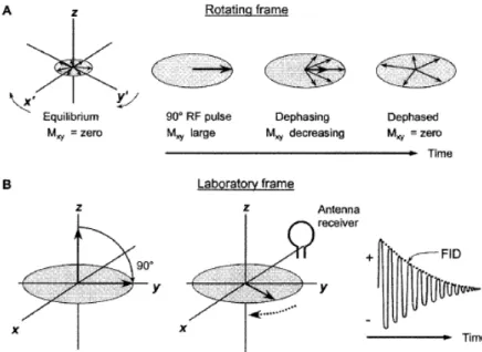
Figure 2.1: A: Conversion of longitudinal magnetization, Mz, into transverse magnetization, Mxy,
results in an initial coherence of the phase of the individual spins of the sample. The magnetic moment vector precesses at the Larmor frequency (stationary in the rotating frame) and dephases with time. B: In the laboratory frame, Mxy precesses and induces a signal in an antenna receiver
that is sensitive to transverse magnetization. A free induction decay (FID) signal is produced, oscillating at the Larmor frequency, and decays with time due to the loss of phase coherence. Adapted from [10].
The “decay” of the FID envelope is the result of the loss of phase coherence of the individual spins caused by magnetic field variations. Micromagnetic inho-mogeneities intrinsic to the structure of the sample cause a spin-spin interaction, whereby the individual spins precess at different frequencies due to slight changes in the local magnetic field strength. Some spins precess faster and some slower, resulting in a loss of phase coherence. External magnetic field inhomogeneities aris-ing from imperfections in the magnet or disruptions in the field by paramagnetic or
ferro-magnetic materials accelerate the dephasing process. Exponential relaxation decay, T2, represents the intrinsic spin-spin interactions that cause loss of phase coherence due to the intrinsic magnetic properties of the sample. The elapsed time between the peak transverse signal and 37% of the peak level 1/e is the T2 decay constant (Figure 2.2). Mathematically, this exponential relationship is expressed as follows:
Mxy(t) = M0e−t/T 2 (2.1)
Where Mxy(t) is the transverse magnetic moment at time t for a sample that has
M0 transverse magnetization at t=0. Since e-1=0.37 when t=T2, then Mxy=0.37M0.
Figure 2.2: The loss of Mxy phase coherence occurs exponentially and it is caused by intrinsic spin-spin interactions in the tissues, as well as extrinsic magnetic field inhomogeneities. The exponential decay constant, T2, is the time over which the signal decays to 37% of the maximal transverse magnetization (e.g., after a 90◦pulse). Adapted from [10].
T2 decay mechanisms are determined by the molecular structure of the sam-ple. Mobile molecules in amorphous liquids exhibit a long T2, because fast and rapid molecular motion reduces or cancels intrinsic magnetic inhomogeneities. As the molecular size increases, constrained molecular motion causes the microscopic magnetic field variations to be more readily manifested and T2 decay to be more rapid. Thus large, nonmoving structures with stationary magnetic inhomogeneities have a very short T2 [10].
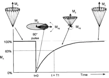
The loss of transverse magnetization (T2 decay) occurs relatively quickly, whereas the return of the excited magnetization to equilibrium (maximum longitudinal mag-netization) takes a longer time. Individual excited spins must release their energy to the local tissue (the lattice). Spin-lattice relaxation is a term given to the expo-nential regrowth of Mz, and it depends on the characteristics of the spin interaction
with the lattice (the molecular arrangement and structure). The T1 relaxation con-stant is the time needed to recover 63% of the longitudinal magnetization, Mz, after
a 90◦pulse (when Mz= 0). The recovery of Mz versus time after the 90◦RF pulse is
expressed mathematically as follows:
Mz(t) = M0(1 − e−t/T 1) (2.2)
Where Mz is the longitudinal magnetization that recovers after a time t in a
material with a relaxation constant T1. Figure 2.3 illustrates the recovery of Mz.
Full longitudinal recovery depends on the T1 time constant.
Figure 2.3: After a 90◦pulse, longitudinal magnetization (Mz) is converted from a maximum value
at equilibrium to zero. Return of Mz to equilibrium occurs exponentially and is characterized by
the spin-lattice T1 relaxation constant. After an elapsed time equal to T1, 63% of the longitudinal magnetization is recovered. Spin-lattice recovery takes longer than spin-spin decay (T2). Adapted from [10].
T1 relaxation depends on the dissipation of absorbed energy into the surrounding molecular lattice. T1 relaxation is strongly dependent on the physical characteris-tics of the tissues - T1 ranges from 0.1 to 1 second in soft tissues, and from 1 to 4 seconds in aqueous tissues and water. Consequently, for solid and slowly moving structures, low-frequency variations exist and there is little spectral overlap with the Larmor frequency [10].
2.3
Spin Echo
Spin echo describes the excitation of the magnetized protons in a sample with an RF pulse and production of the FID, followed by a second RF pulse to produce an echo. The timing between the RF pulses allows separation of the initial FID and the echo and the ability to adjust tissue contrast.
An initial 90◦pulse produces the maximal transverse magnetization, Mxy, and
places the spins in phase coherence. The signal exponentially decays due to in-trinsic and exin-trinsic magnetic field variations. After a time delay of T E/2, where
TE is the time of echo, a 180◦RF pulse is applied, which inverts the phase of the spin system and induces a rephasing of the transverse magnetization. The spins are rephased and produce a measurable signal at a time equal to the TE. This sequence is depicted in the rotating frame in Figure 2.4.
Figure 2.4: The spin echo pulse sequence starts with a 90◦pulse and produces an FID signal that decays according to T2*. After a delay time equal to T E/2, a 180◦RF pulse inverts the spins
and reestablishes phase coherence, producing an echo at a time TE. Effects of inhomogeneities of external magnetic fields are canceled, and the peak amplitude of the echo is determined by T2 decay. The rotating frame shows the evolution of the vector in the opposite direction of the FID. Adapted from [10].
Just before and after the peak amplitude of the echo (centered at time TE), digital sampling and acquisition of the signal occurs. Spin echo formation separates the RF excitation and signal acquisition events by finite periods of time, which em-phasizes the fact that relaxation phenomena are being observed and encoded into the images. Contrast in the image is produced because different tissue types relax differently (based on their T1 and T2 characteristics).
Multiple echoes generated by 180◦pulses after the initial excitation allow the de-termination of the “true” T2 of the sample. Signal amplitude is measured at several points in time, and an exponential curve is fit to this measured data (Figure 2.5). The T2 value is one of the curve-fitting coefficients.
Figure 2.5: “True” T2 decay is determined from multiple 180◦refocusing pulses. While the FID envelope decays with the T2*- decay time resulting from both intrinsic and extrinsic magnetic field variations, i.e. MR contrast materials, paramagnetic or ferromagnetic objects – decay constant, the peak echo amplitudes of subsequent echoes decay exponentially with time, according to the T2 decay constant. T2 is always longer than T2*. Adapted from [10].
Contrast in an image is proportional to the difference in signal intensity between adjacent pixels in the image, corresponding to two different voxels in the subject.
2.4
T2-weighted image
A “T2-weighted” (T2W) spin echo sequence is designed to produce contrast chiefly based on the T2 characteristics of tissues by de-emphasizing T1 contribu-tions. This is achieved with the use of a long Repetition Time (TR) to minimize the differences in longitudinal magnetization during the return to equilibrium, and a long TE to accentuate T2 differences during signal acquisition. Compared with a T1-weighted image, inversion of tissue contrast occurs, because short-T1 tissues usually have a short T2, and long-T1 tissues have a long T2. Tissues with a long T2 maintain transverse magnetization longer than short-T2 tissues, and thus present higher signal intensity. As TE is increased, more T2 contrast is achieved, at the expense of a reduced transverse magnetization signal.
2.5
Steady-State Precession
Steady-state precession refers to equilibration of the longitudinal and transverse magnetization from pulse to pulse in an image acquisition sequence. In all standard image techniques (e.g., spin echo), the repetition period TR of RF pulses is too short to allow recovery of longitudinal magnetization equilibrium, and thus partial satu-ration occurs. When steady-state partial satusatu-ration occurs, the same longitudinal magnetization is present for each subsequent pulse. For very short TR, less than the T2* decay constant, persistent transverse magnetization also occurs. During each pulse sequence repetition, a portion of the transverse magnetization is converted to longitudinal magnetization and a portion of the longitudinal magnetization is converted to transverse magnetization. Under these conditions, steady-state longi-tudinal and transverse magnetization components coexist at all times in a dynamic equilibrium. Steady-state imaging is practical only with short and very short TR. In these two regimes, flip angle has the major impact on the contrast “weighting” of the resultant images [10].
2.6
Cardiac Magnetic Resonance
MRI is used to make images of various organs of the human body, and specifically Cardiac Magnetic Resonance (CMR) imaging has emerged as a robust medical imag-ing technique for the non-invasive investigation of cardiovascular system function, structure and disorders. This MRI branch uses the same basic principles as MRI with the combination of rapid imaging techniques or sequences. CMR allows for the possibility of electrocardiography (ECG) gating and synchronization that enhances the quality of the images of the cardiovascular system by minimizing cardiac motion artifacts. With these optimizations, morphological structures and key functions of the cardiovascular system can be visualized and measured. The possibilities that the new applications allow, have created great enthusiasm in the CMR community. However due to the low number of studies yet performed, there is some uncertainty regarding its possible clinical applications. One of the possibilities that CMR opens
up is to provide a comprehensive assessment of cardiovascular disorders in a single session. Due to this, CMR represents a very important method of evaluation for the cardiac function and perfusion and can be used for many purposes in cardiology. Apart from these applications, an exceptional advantage of CMR is the capacity to do an exhaustive myocardial tissue characterization [11].
CMR is the only non-invasive imaging technique that can detect myocardial edema, which is believed to be a fundamental response to ischemia reperfusion injury. This has traditionally been performed with water-sensitive T2-Weighted (T2W) imaging, under the principle that prolonged T2-relaxation time due to in-creased mobility of water protons in edematous myocardium results in inin-creased T2 signal intensity.
Studies in animals and patients have demonstrated that increased myocardial T2 may be associated not only with acute myocardial infarction (MI), but also with severe transient myocardial ischemia [12]. Elevated myocardial T2 is also known to accompany myocarditis, cardiac allograft rejection and sarcoidosis, among other conditions [2]. This relationship makes T2 and T2W imaging very useful in CMR and can be clinically helpful to differentiate acute from chronic myocardial lesions and to detect even small acute myocardial damage very early [13]. Differences in myocardial T2 relaxation should reflect differences in the underlying tissue charac-teristics.
These and other studies using T2 to characterize pathological changes in my-ocardium have relied on T2W imaging with a black-blood (BB) turbo spin echo technique [14]. Traditional BB turbo spin echo-based T2W imaging is limited by a set of challenges which continue to affect its diagnostic utility (Figure 2.6) and impede its widespread clinical acceptance: i) phased-array coils cause regional my-ocardial signal variation that can lead to inaccurate interpretation and diagnosis – thus specialized normalization methods are required; ii) high/bright signal from stagnant blood makes it difficult to differentiate edema from sub-endocardial blood; iii) myocardial signal loss caused by through-plane motion; and iv) the qualitative nature of T2W imaging where interpretation depends on regional differences in my-ocardial signal intensity, which may vary depending on sequence parameters (e. g. TE, slice thickness). In patients with irregularities in cardiac rhythm or difficulties with breath holding, artifacts can increase.
In order to solve these problems, semi-quantitative approaches have been devel-oped for T2W-CMR that, for instance, compute signal intensity relative to unaf-fected remote myocardium or adjacent skeletal muscle. However, these approaches perform poorly when there is diffuse myocardial involvement. Furthermore, these may be insensitive when there is concomitant skeletal muscle involvement, which has been reported in myocarditis [15].
Figure 2.6: A: Acute myocardial infarction (MI) patient, with significant RR variability, exhibit-ing edema with false-positive black-blood (BB) turbo spin-echo showexhibit-ing apparently elevated T2 in the left anterior descending (incorrect) coronary territory. B: Patient with chronic MI in the left anterior descending territory showing a false-positive BB turbo spin-echo suggesting edema. C: Example illustrating bright-blood artifact for BB turbo spin-echo image resulting from stagnant blood within trabeculae along the endocardial wall. Adapted from [16].
Therefore alternatives for more stable detection and easier quantification of edema are clinically warranted. An alternative approach to T2W imaging, which overcomes many of these limitations, is to directly quantify the T2 of the my-ocardium – quantitative T2 mapping.
2.7
T2 mapping
In recent years, new ‘mapping’ techniques have been proposed to allow for quan-titative CMR. The majority of these sequences are normally single-slice breath-hold (BH) acquisitions. Using such mapping techniques, instead of generating ‘weighted’ images, a colored pixel map is produced where each pixel corresponds to the T1, T2 or T2* value (Figure 2.7). With the right contrast agent, it is also possible to
use these maps to analyze the interstitium (e.g. amyloid, edema or fibrosis) and evaluate the extracellular volume (ECV) [17].
Figure 2.7: T2 mapping in healthy volunteer demonstrates a homogeneous T2 distribution. Mid-ventricular short-axis (SAX) slice through the left ventricle (LV) shows homogenous T2 values throughout the myocardium. It is also possible to see the right ventricle (RV). In this study the average myocardial T2 value was 40.5 ± 3.3 ms. Adapted from [18].
T2 mapping is based on several snapshot images with different TEs (T2 weight-ing) and a map is generated that gives T2 time in absolute value for every single pixel. In a colour-coded scale, the map directly displays absolute T2 values for any single pixel that can be assessed globally or for any segment or region of interest (ROI). The map can be acquired in any orientation and is independent from coil proximity.
There are 2 main types of T2 mapping techniques: spin-echo-based and T2-preparation (T2prep) steady-state free-precession (SSFP)-based techniques. How-ever, since the T2 mapping techniques based on spin-echo sequences are sensitive to ghosting and motion artifacts (induced by cardiac arrhythmias or imperfect BH), the latter are generally preferred in CMR [3].
Normally, a T2prep SSFP sequence [16] is used to generate three T2W images – the minimum required for an exponential fit and to minimize BH duration and patient discomfort – each one with a different T2prep time. Because these images are acquired in the transient state of single-shot SSFP immediately after the T2prep pulse, the primary source of contrast is the T2 relaxation time. Thus, the signal in each image represents a different TE along the T2 decay curve.
The design of this sequence incorporates non-selective composite pulses for in-sensitivity to motion and B0 and B1 inhomogeneities and the SSFP readout module
is usually applied immediately after the T2prep module to sample the magnetization prior to it reaching the steady state.
Parametric maps are generated by fitting the measured signal in each pixel to the following two-parameter (M0 and T2) exponential equation:
S(x, y) = M0(x, y)e−T ET 2prep/T 2(x,y) (2.3)
where S(x,y) is the measured signal intensity, M0(x,y) is a lumped parameter
that includes the equilibrium magnetization and local receiver coil sensitivity, and TET2prep is the T2prep echo time (Figure 2.8). Those TET2prep times are chosen
based on the expected range of T2 values in the myocardium – recent work has shown that the T2 for normal myocardium is approximately 55 ms [4]. Longer TET2prep than the T2 for normal myocardium can cause significant signal loss.
Using quantitative T2 mapping, the artifacts associated with T2W imaging may be minimized, image contrast dependency on user-defined parameters and subjec-tive interpretation can be reduced, and subtle T2 differences between tissues may be more easily detected. Also the quantitative approach is independent of the heart rate, and has low interscan variability rates [19]. The quantification of T2 offers a distinct advantage in the detection of global changes, in comparison with T2W imaging, which relies on regional differences in myocardial signal.
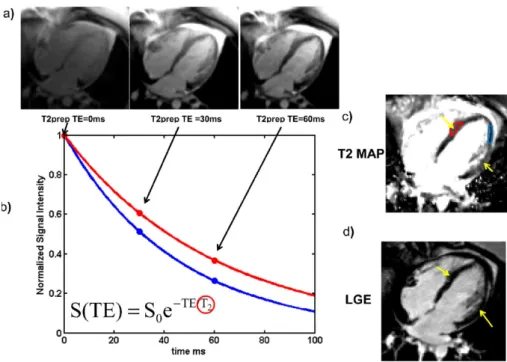
Figure 2.8: Calculation of T2 maps using a T2prep pulse sequence in a patient with atypical Takusubo cardiomyopathy. (a) Multiple images with T2 preparations with different TE are ac-quired. As the TE is increased for this spin-echo-based preparation, the myocardial signal intensity decreases due to T2 decay. (b) A T2 decay curve is fit to the data of each pixel, with pixels with longer T2 (red curve) decaying more slowly than regions with shorter T2 (blue curve). (c) The T2 map shows a region of edema (yellow arrows and red region of interest (ROI)) in this patient. (d) The absence of late gadolinium enhancement (LGE) confirms the diagnosis of atypical Takusubo cardiomyopathy. Adapted from [3].
Quantitative T2 mapping addresses the limitations of qualitative T2W imaging and provides a practical, promising and accurate method of assessing myocardial edema associated with acute ischemia, infarction, and other pathological conditions affecting myocardial water content and showing promise for application in clinical practice. The lack of sensitivity to field inhomogeneities makes T2 mapping a good strategy for the detection of regional hemodynamic differences in the heart. To per-form T2 mapping, a cardiac imaging method that would provide high T2 contrast, high signal-to-noise ratio (SNR), and low motion sensitivity is thus highly desirable.
As with T1 mapping, global diseases such as pan-myocarditis may be identified by T2 mapping, and preliminary results showing this in several rheumatologic dis-eases (lupus, systemic capillary leak syndrome) and transplant rejection, detecting early rejection missed by other modalities [5].
2.8
T2 preparation module
The most common approach for achieving T2 weighting for T2 mapping in CMR uses the T2prep module. A magnetization-prepared, T2W sequence is used to sup-press muscle and venous structures. When combined with lipid supsup-pression, this technique improves the visualization of the coronary arteries. The T2prep module is shown in Figure 2.9 and was designed to store T2W magnetization along Mz in a
manner that is robust in the presence of flow as well as B0 and B1 inhomogeneities
followed by a train of 180y◦pulses, which are equally separated. After the refocusing
pulses a 90x◦tip-up pulse is performed to return the transverse magnetization to
the longitudinal axis, followed by a spoiler gradient (SPGR) to destroy any residual transverse magnetization.
Figure 2.9: T2prep sequence illustrated with four refocusing pulses.
The T2 weighting generated by this module suppresses muscle because the T2 of muscle is much shorter than that of oxygenated blood (e. g. T2oxygenated blood = 290
ms, T2myocardium = 40 ms) [20]. After the application of the first 90◦RF pulse of the
T2prep module, the Mxy◦magnetizations of the vessel wall and fat decay faster than
that of blood because of their shorter T2 relaxation time, thereby increasing the contrast between them. Conveniently, the T2 of oxygenated blood is also greater than that of venous blood which improves contrast between oxygenated and de-oxygenated blood.
2.9
Respiratory Navigators and Motion
Cor-rection
Respiratory navigators are incorporated into the MRI pulse sequence and can be used to monitor the respiratory movement and deformation of the heart and surrounding tissues and organs (Figure 2.10).
Figure 2.10: Respiratory motion can cause different effects. Craniocaudal respiratory motion of the diaphragm and abdominal organs (e.g. liver and spleen) can produce blurring in the top of the abdomen and in the liver (see arrow in image (a)) and ghost images of these organs (see arrow in image (b)). Temporal modulation of the magnitude and phase of the transverse magnetization, as tissues move from voxel to voxel, are the responsible for these effects. Adapted from [21].
Respiratory navigators are normally real-time image acquisitions, which are in-terleaved with the high resolution MR sequence, allowing snap-shots of one or more motion dimensions of the respiratory state before or after each segmented k-space acquisition.
Ehman et al. [21] in the end of the 1980’s proposed the first respiratory di-aphragmatic one-dimension navigator (d1D NAV) which was obtained on the top of the right hemi-diaphragm, determining the foot-head (FH) motion of the lung-liver interface to correct for the respiratory motion of the liver. Due to its characteristics – it can be used with a large amount of cardiovascular imaging sequences, it is easy to use and allows a very accurate tracking of the lung-liver interface – this became a very popular way to assess the respiratory motion for CMR [6]. Also the possibility of prospective real-time motion compensation, because of the time of acquisition and processing being relatively short (around 10-30 ms), is a major advantage of the d1D NAV. In addition to this, as the respiratory motion is mainly perpendicular to the lung-liver interface (i.e. in the FH direction) with the d1D NAV approach the motion can be followed with very good precision.
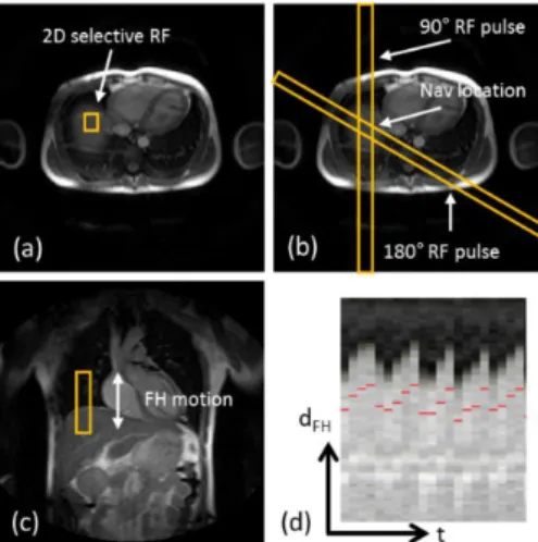
The d1D NAV can be implemented using two alternative approaches: a spin-echo implementation where the 90◦RF excitation and 180◦RF refocusing pulses are obliquely aligned (the overlapping zone is the d1D NAV volume) or a pencil beam navigator – 2D RF excitation pulse with a SPGR echo read-out in the orthogonal direction. Figure 2.11 shows scan planning for the two approaches, as well as the resulting d1D NAV signal also represented over time, where it is possible to see the respiratory motion between the lung and the liver. However, hysteresis between the diaphragm and the heart respiratory motions between inspiration and expiration, and the necessity of a motion model to estimate the respiratory motion of the heart (indirectly measured using the diaphragm movement information), are the main limitations of the d1D NAV.
Figure 2.11: Scan planning of d1D NAV in axial plane using either a 2D selective RF “pencil beam” excitation (a) or a spin-echo approach with obliquely aligned 90◦excitation and 180◦refocusing pulses (b). The d1D NAV is located on the dome of the right hemi-diaphragm with the read out in the foot-head (FH) direction (c). The d1D NAV signal (d) clearly shows the displacement of the lung-liver interface along the FH direction (dFH) over time (t). Adapted from [6].
Additionally, for using the d1D NAV it is necessary to do scan planning and also define separate imaging parameters for the navigator acquisition, which increases the scan complexity making it an inherent limitation. In order to address these disadvantages, a new technique for respiratory motion compensation has been pro-posed: so called self-navigation (Figure 2.12) [7]. It consists of an estimation of the respiratory motion directly from the MR data, respecting certain conditions: the central line of k-space is measured at least once per k-space segment and in order to maximize the accuracy of the respiratory motion, the readout must be in line with the FH direction. With this technique, the problems associated with hysteresis among diaphragmatic and heart motion do not exist because the respiratory motion is directly measured instead of resorting to a motion model [8].
Figure 2.12: Reformatted images of the right coronary acquired with the d1D NAV technique (a, c) and with the self-navigation (b, d). In (a) and (b) the proximal and the distal part of the right coronary artery are highlight with the white arrows. It can be observed that with self-navigation the vessel sharpness and length are increased. The white arrows in (c) and (d) highlight regions where the self-navigation showed an improved delineation of the coronary vessels where similar image quality was obtained with both approaches. Adapted from [7].
Normally, static tissue (e.g. chest wall) is present in the navigator image because self-navigation images are acquired as 1D projections of the FOV, so the motion es-timation performance of the navigator can become compromised. To overcome this limitation, a combination of this method with spatial encoding has been proposed which separates moving from static tissue, which is called image-based navigation (iNAV).
In iNAV single two-dimensional (2D), orthogonal 2D, or three-dimensional (3D) [9] real-time images are acquired in every heart-beat preceding the main MR ac-quisition (Figure 2.13). With this technique it is possible to improve the quality of the respiratory motion estimation because the moving heart can be spatially iso-lated from surrounding static tissues. Beside this advantage, image-based motion compensation has extra degrees of freedom for motion correction, and so rotation and non-rigid motion correction are also possible – not limited to only translational motion in numerous directions. However, the navigator acquisition can saturate the magnetization or artifacts may be present in the subsequent and spatially overlap-ping MR acquisition, when the iNAV is used. A solution may be placing the MR acquisition before the navigator image, so called trailing navigator, but this cannot be combined with prospective respiratory gating and correction. When iNAV is compared with 1D navigators (e.g. d1D NAV or self-navigation), it is easy to imag-ine that those real-time implementations are much more challenging, due to the augmented computational complexity of multi-dimensional image reconstruction, registration and correction. The downside of iNAV compared to self-navigation, is that extra scan planning is required to define the navigator image location, because the navigator is not easily extracted from image acquisition.
Figure 2.13: 3D segmented k-space CMR angiography sequence using iNAV for prospective motion correction. Image (a) is the reference and the template is extracted from it. After that it is utilized to estimate 2D motion in the shots (b) and (c). Prior to each acquisition, the position of the 3D image is updated using this information. Adapted from [9].
As previously stated, image-based approaches have been suggested to improve motion estimation, by spatially encoding in 2D or 3D [22], which enables the possi-bility to separate the static chest from the moving heart. However, Henningsson et al. [23] created a 2D self-navigator (2DSN) which acquires images by encoding the startup profiles of a balanced SSFP sequence, which are principally used to catalyze the magnetization towards the steady-state. This makes possible the translational correction in the frequency and phase encoding directions and makes possible the separation of static and moving structures. In this approach a template matching algorithm was used to estimate the respiratory motion from the 2DSN and during the image reconstruction the data is retrospectively corrected. With this approach the FH and left-right (LR) motion are calculated and retrospective translational motion correction performed.
In this approach, the 2DSN image resolution in the phase encoding direction is a function of the number of startup profiles. All 2DSN are reconstructed to the same matrix size irrespective of the phase encoding resolution. The 3D imaging volume is oriented in the coronal plane with frequency encoding in the FH direction and phase encoding in the LR direction. In order to increase the 2DSN resolution and at the same time diminish the duration of the 2DSN, a half Fourier acquisition with a factor of 0.6 in the phase encoding direction can be used [24]. As the acquisition of iNAV center of k-space should be as close to the 3D image acquisition as possi-ble, the 2DSN sequence is implemented with a high-low profile order. Also, along the slice selection direction no phase encoding is needed and so 2DSN images are projections of the field-of-view (FOV) in the anterior-posterior direction.
In the CMR sequence, it is possible to create image contrast by using prepulses such as fat saturation or T2prep (used for T2 mapping). The number of startup profiles determines the time between prepulses and imaging and so it is desirable to minimize this time. Also k-space data is modulated with a linear phase – in the image domain it represents a translational shift – so the motion correction can be applied to the CMR retrospectively. The phase shift ϕA introduced by the motion
along encoding direction A can be calculated for the shot s, as:
ϕA(s) = (2π · ∆A)/F OVA (2.4)
where ∆A is the displacement estimation as measured by the navigator, and FOVAis the field of view. The phase modulation is applied to each complex k-space
data point kj, where j is the index in k-space along encoding direction A, acquired
in shot s as described by
kj = kj · e(i·ϕA(s)·j) (2.5)
For the above mentioned correction techniques the phase shift is calculated for every shot in the frequency encoding direction.
Henningsson et al. [23] concluded that with their 2DSN the image quality of CMR was improved compared to a d1D NAV with a FH tracking factor of 0.6. Ten
startup profiles were shown to be sufficient for 2DSN motion correction and to gen-erate CMR with excellent image quality.
2.10
T2 mapping – State of the art
Over the past 25 years a number of in vivo studies have measured the T2 of healthy human myocardium, primarily using techniques based on spin echo acquisi-tions. These methods are time-consuming and prone to the same motion sensitivity that has plagued T2W imaging of the heart. Also, T2 mapping techniques based on BB turbo spin echo sequences are sensitive to ghosting and motion artifacts [3].
Myocardial T2 mapping techniques using T2prep SSFP have been described by Huang et al. [25] for blood oxygenation level-dependent (BOLD) imaging – which is the detection of local T2 or T2* changes in the myocardium in response to a
va-sodilatory challenge. A combined T1 and T2 mapping method by Blume et al. [26] for differentiation of acute from chronic MI was proposed. Blume et al. [26] showed that myocardial T2 estimation is improved by including an image without T2prep (TE = 0 ms). While these were promising initial studies, neither investigated the potential for T2 mapping to address the known limitations of T2W imaging caused by residual blood signal, surface coil intensity variation, and myocardial motion ar-tifact.
In 2009, Giri et al. [4] introduced a direct T2 mapping for quantitative mea-surement of T2 relaxation time, using T2prep SSFP and showed improved results compared with the conventional T2W (Figure 2.14). Giri et al. have demonstrated an accurate, fast, quantitative approach to detect the elevated T2 associated with myocardial edema that successfully addresses the limitations of T2W imaging.
Figure 2.14: Mid-ventricular short-axis and vertical long axis images from a patient. Coronary angiography confirmed >90% occlusion of right coronary. The infracted region could not be de-tected in T2prep SSFP image with T2prep = 55 ms (column 1). T2 maps (column 2) demonstrate increased T2 in the inferior regions and the endocardial borders are clearly demarcated. Late Gadolinium Enhancement (LGE) images (column 3) show the location and extent of the infarct. S = Signal Intensity. Adapted from [4].
In this approach, a T2-prepared SSFP sequence was used to produce three T2W images, one each with different T2prep times (TET2prep = 0, 24 and 55 ms). The
principal source of contrast is the T2 relaxation time because these images are ob-tained in the transient state of single-shot SSFP immediately after the T2prep pulse. The SSFP readout module was applied immediately after the T2prep to sample the magnetization prior to reaching the steady state. A wait time of 2 RR intervals was introduced between the images to allow for relaxation of longitudinal magnetization. Therefore, a total of 7 RR intervals were necessary to get the three T2prep images. The sequence timing was adjusted for each T2prep time to guarantee that the SSFP readout was always timed to the same phase of the cardiac cycle.
Many studies were performed based on this sequence and they have shown that T2 mapping can detect edematous myocardial territories in a variety of cardiac pathologies, including acute MI [19] and it also has been used to identify iron over-load [27]. Verhaert et al [28] assessed T2 mapping in patients with acute MI and found that myocardial segments characterized by recent ischemic injury can be quan-titatively differentiated from remote myocardium by their higher T2 value. Another study from the same group [5] showed the usefulness of T2 mapping in suspected myocarditis or tako-tsubo cardiomyopathy, demonstrating that T2 mapping can identify myocardial involvement beyond conventional CMR techniques such as T2W and Late gadolinium enhancement (LGE) imaging. T2 mapping has also been used as a non-invasive tool for cardiac transplant monitoring with promising preliminary findings in small cohorts and also shown to be a potential non-invasive tool for char-acterizing rejection in cardiac allografts [29]. Finally, T2 mapping might help to improve tissue characterization in the case of intracardiac tumour but more expe-rience across various tumour entities is needed to assess the clinical utility of T2 mapping for tumour differentiation [30].
Unfortunately, these T2 mapping techniques exhibit heart-rate dependency, sen-sitivity to the order of acquisition and flip angle, incomplete T1 recovery resulting in T1 weighting and errors in the T2 relaxation time measurements [31]. Also, with this technique, T2 maps are typically acquired as one or several 2D slices, while the underlying pathologies often have a complex 3D structure. In addition, a 3D approach should sample considerably more myocardial tissue per unit time than a 2D approach, and might thus increase the precision of T2 determination – the 2D approaches have limited in-plane resolution [4], [28].
The value of higher field strength for clinical imaging has previously been demon-strated for selected CMR applications and is mostly due to the higher SNR and thus higher spatial and temporal resolution, which allow for improved sensitivity and specificity [32]. For the first time, van Heeswijk et al. [33] validated a free-breathing radial gradient echo T2 mapping technique at 3T, demonstrating its accuracy and reproducibility in comparison to a BH BB T2W fast spin echo technique. van Heeswijk et al. [18] also achieved 3D T2 maps at 3T using a 3D radial acquisition in combination with golden step-based self-navigation. Using a bSSFP sequence with 20% undersampling resulted in isotropic images (1.7 mm3). Imaging every
other heartbeat recovered SNR, and the residual influence of T1 was corrected by an empirical factor applied during fitting. All data acquired were used, and 3D affine warping of volumes at different respiratory positions was used in final image reconstruction.
van Heeswijk et al. tested it in a small group of 11 patients where comparisons were made regarding the extent of edema assessed by conventional T2W images and T2 maps at 3T (Figure 2.15). This technique allows for the 3D characterization of edema in established cardiovascular disease in less than 20 minutes and the perfor-mance of this 3D T2 mapping approach appears to be a robust tool for myocardial edema at 3T as well as at 1.5T.
Figure 2.15: Short-axis (SAX) slices and 3D volume renderings of the 3D T2 maps in three pa-tients with cardiovascular diseases. a, b: A patient with a subacute MI. A region with significantly elevated T2 can be identified (arrows). c, d: A patient with myocarditis. Several small regions of T2 elevation can be discerned (arrows). e, f: A patient with a cardiac graft and no rejection as seen in endomyocardial biopsy also demonstrates the absence of subendocardial elevated T2 values, although a small patch with elevated T2 can be observed at the anterior epicardium (arrow). g: A region of elevated T2 can be observed in a control 2D T2 map at the same level as (c). However, the region is mostly epicardial and not transmural, which causes it to appear smaller in the 3D subendocardial segmentation. h: A control 2D T2 map at the same level as (e). The blue patch is a nonmapped signal void. Adapted from [18].
van Heeswijk et al. work represents a significant contribution to the techni-cal developments in parameter-mapping techniques. Specifitechni-cally, their investigation provided further improvement to the assessment of myocardial edema beyond con-ventional T2W fast spin echo sequences or bright-blood T2prep module SSFP tech-niques. Techniques based on T2W SSFP are sensitive to susceptibility artifacts and large RF inhomogeneities affecting image quality. The need for longer BH times to enable T1 recovery between T2prep modules may also be a challenge for the clin-ical applicability of 3T CMR edema imaging. The introduction of free-breathing T2 mapping segmented k-space radial gradient echo may not only overcome some of the limitations described, but it may also provide a tool for accurate quantita-tive assessment of the change in tissue composition at 3T and to specifically assess myocardial edema. Mapping experiments in volunteers at 3T demonstrated that at higher field strengths myocardial T2 can be assessed with low intra- and inter-observer variability [34].
More recently, Ding et al. [17] developed a free-breathing 3D T2 mapping method based on the saturation-prepared, T2prep RF-SPGR echo sequence, which achieves high spatial resolution T2 maps with whole-heart coverage (Figure 2.16). Compared
with previous T2 mapping methods, this sequence is 1) less dependent on field ho-mogeneity (obtained by using SPGR and partial echo readout), 2) highly efficient (by utilizing all heartbeats for imaging and requiring no T1 recovery time), 3) mo-tion compensated (via respiratory navigators), 4) insensitive to heart rate variamo-tion (by using a “reset” nonselective saturation prepulse), and 5) intrinsically spatially registered by interleaving volumes with different T2prep. Also, the 3D acquisition improved both through-plane motion compensation and SNR compared with previ-ous techniques.
Figure 2.16: a: Pulse sequence diagram for the free breathing 3D T2 mapping sequence. Three or more differentially T2-weighted (T2W) volumes were acquired in an interleaved fashion. Each volume was respiratory navigator gated, ensuring coregistered images. A SAT pulse was applied at the start of every heartbeat to reduce variations in signal intensities. To prevent changing heart rates from affecting the degree of T1-weighting in the images, the TSAT (SAT delay, duration
between SAT and T2 Prep) was kept constant even when the Ttrigger(trigger delay, imaging delay
after ECG R wave is detected) was allowed to change to maintain imaging during diastole in the presence of heart rate variability. The same navigator template was used for detection of motion across all volumes, ensuring coregistration. If a given heartbeat was rejected due to respiratory motion, data were reacquired immediately until an appropriate level of motion was achieved before proceeding to the next volume’s data. b: Sample images from three acquired 3D volumes yielded voxel-by-voxel 3D T2 maps (c). Adapted from [17].
Finally Yang et al. [35] developed a time-efficient, free-breathing, whole heart T2 mapping technique at 3T with hybrid radial-cartesian trajectory. ECG-triggered 3D images were acquired with different T2 preparations at 3T during free breath-ing. Respiratory motion was corrected with a navigator-guided motion correction framework at near perfect efficiency and image intensities were used to fit a mono-exponential function to derive myocardial T2 maps. Yang et al. concluded that the proposed whole heart T2 mapping approach could be performed within 5 min with similar accuracy to that of the 2D BH T2 mapping approach.
Although, T2 maps can easily be acquired with higher hearts rates, in arrhyth-mias and also in other conditions when T2W imaging fails and allows for global and regional assessment of myocardial tissue properties, further technical improvements - e.g. the effects of scan time shortening techniques on the performance of T2 map-ping - are expected to advance their clinical application in the detection of acute, subacute, and subclinical pathologies.
In so far T2 mapping represents a very promising tool for real world CMR in the acute clinical setting and has already demonstrated clinical usefulness as a quantita-tive tissue characterization MR technique in a variety of common cardiac conditions. T2 mapping appears to be a useful confirmatory test for conventional T2W imaging and is an emerging topic with the potential to become a powerful tool in the iden-tification and quaniden-tification of diffuse myocardial processes without biopsy. Early evidences suggest that this technique detects initial stage disease missed by other imaging methods and has potential for prognosis, as a surrogate endpoint in clinical trials and also to monitor therapy.