Determinants of bank capital ratios in European Union banks

M

ASTER

F

INANCE

M

ASTER

’

S

F

INAL

W

ORK

D

ISSERTATION

D

ETERMINANTS OF

B

ANK

C

APITAL

R

ATIOS IN

E

UROPEAN

U

NION

B

ANKS

V

ANESSA

M

IGUEL

T

OSCANO

M

ASTER

F

INANCE

M

ASTER

’

S

F

INAL

W

ORK

D

ISSERTATION

D

ETERMINANTS OF

B

ANK

C

APITAL

R

ATIOS IN

E

UROPEAN

U

NION

B

ANKS

V

ANESSA

M

IGUEL

T

OSCANO

S

:

P

D

J

M

S

A

BSTRACT

We analysed European Union banks’ Common Equity Tier 1 (CET1) ratio determinants after Sovereign Debt Crisis. We resorted to information from the

Bankscope database. We exported information of 137 banks from the 27 countries

belonging to the EU, from 2011 to 2018. We performed a regression analysis, running several models to identify the significant variables and their impact on the CET1 ratio. To attest the results’ robustness, we replicate the analysis winsorizing the dependent variable and the variable that represents Return on Equity. We verified that size, risk exposure, leverage and liquidity are factors that affect CET1 ratio and banks solvency. Additionally, we observed that the European Central Banks’ (ECB) asset purchase program seems to increase banks’ capacity to absorb potential losses, which justifies this kind of measures by the regulator.

JEL Classification: G01; G20; G21

Keywords: CET1 ratio; CET1 ratio determinants; Basel III; Capital

R

ESUMO

Neste trabalho, analisamos os determinantes do rácio Common Equity Tier 1 (CET1) dos bancos da União Europeia após a Crise das Dívidas Soberanas. Utilizámos informação da base de dados do Bankscope. Exportámos informação de 137 bancos dos 27 paises da UE no período de 2011 a 2018. Baseámos o nosso estudo numa análise de regressão, sendo que analisámos vários modelos de forma a analisar od determinantes e qual o seu impacto no rácio CET1. Para atestar a robustez dos resultados, replicámos a análise aplicando um processo winsor à variável dependente e à variável que representa o Return on Equity. Verificámos que o tamanho, a exposição ao risco, a alavancagem e a liquidez são fatores que afetam o rácio CET1 e consequentemente a solvabilidade do banco. Adicionalmente, observámos que o programa de compra de ativos por parte do Banco Central Europeu (BCE) aparenta aumentar a capacidade dos bancos para absorver as suas potencias perdas, pelo o que se justifica este tipo de ações por parte do regulador.

Classificação JEL: G01; G20; G21

Palavras-chave: Rácio CET1; Determinantes do rácio CET1; Basileia III;

A

CKNOWLEDGEMENTS

I would never be able to finish this dissertation if I hadn’t received support and motivation from some people.

First, I would like to thank my father, Luis Toscano, and my mother, Lurdes Toscano, for making such an investment in my education, for always believing in me and for the values they gave me. Thanks to you I never quit, and I am driven by the desire of making you as proud of me as I am of you.

To my sisters, Inês and Diana, that I hope to feel inspired by me. Never give up your dreams and keep fighting for them!

To my supervisor, Professor Joaquim Sarmento that followed and guided me during all the process. To Professor Vítor Barros that helped me at the beginning of this dissertation.

I would like to thank my boyfriend Tiago for having the patient needed to put up with me. Thank you for all the help, love and motivation from the beginning until the very end.

I thank my closest friends for the strength given when I felt less confident. Finally, I thank my colleagues (and friends) that worked with me when I was developing this thesis. Thank you for being so flexible and for all the suggestions and motivation given.

This dissertation is the product of a huge personal effort that without the support received it wouldn’t be possible. I am very lucky, thank you all!

T

ABLE OF

C

ONTENTS

2.1. European debt crisis ... 3

2.2. Causes and consequences ... 5

2.3. Crisis effects ... 7

2.4. Measures taken ... 7

2.5. Basel III ... 9

2.6. Capital ratios ... 11

2.6.1. Capital ratios: main findings ... 12

3. Data and methodology... 13

3.1 Sample ... 13 3.2 Dependent variable... 13 3.3 Independent variables... 15 3.4 Regression model ... 17 3.4.1 Preliminary statistics ... 18 3.5 Robustness analysis ... 21 4. Results ... 22

4.1 Determinants of CET1 ratio ... 22

4.2 Robustness analysis results ... 25

5. Conclusion ... 27

References ... 28

L

IST OF

F

IGURES

Figure 1- Standardized normal probability plot ... 40

Figure 2- Shapiro-Wilk test output ... 40

Figure 3- Kernel density graph ... 41

Figure 4- Standardized normal probability plot (Robustness check) ... 41

Figure 5- Kernel density graph (Robustness check) ... 41

Figure 6- Residuals histogram (Robustness check) ... 41

Figure 7- Dependent variable's Histogram ... 41

Figure 8- Residuals histogram ... 41

L

IST OF

T

ABLES

Table II - Determinants of CET1 Ratio ... 24

Table III - Determinants of CET1 Ratio (Winsorized) ... 26

Table IV - Literature Review Summary Table of Empirical Papers ... 33

Table V - Literature Review Summary Table of Independent Variables ... 38

Table VI - Descriptive statistics ... 40

Table VII - Correlation matrix ... 40

L

IST OF

A

BBREVIATIONS

CET1- Common Equity Tier 1 EU- European Union

ECB- European Central Bank EBF- European Banking Federation

MREL- Minimum Requirement for own funds and Eligible Liabilities M&A- Merger and Acquisitions

GDP- Gross Domestic Product EBA- European Banking Authority RWA- Risk-Weighted Assets ROA- Return on Assets ROE- Return on Equity

GLS- Generalized Least Squares OLS- Ordinary Least Squares GLM- Generalized Linear Model

1. I

NTRODUCTION

The recent financial crisis affected the entire financial system. Regulatory measures were implemented as a response to the deficiencies detected. Given that certain European countries were facing weak economies, the financial crisis worsened their situation. Highly indebted countries in Europe affected the banking sector, leading to the European sovereign debt crisis. Bank capital ratios can detect banks’ incapability to absorb losses (BCBS, 2016).

Common Equity Tier 1 Ratio, hereafter CET1 ratio, is an example of a bank capital ratio. It indicates banks’ capacity to absorb losses, which makes important to address its determinants. Identifying the factors that influence this capital ratio will allow us to use this information. According to the Basel III regulatory framework, this ratio should meet a minimum of 4,5% (Basle Committee on Banking Supervision, 2017).

Currently, European banks have 13.8%, on average, as reported by EBF1. Still, due to the difficulties faced, the Single Resolution Board requires the establishment of Minimum Requirement for own funds and Eligible Liabilities (MREL) (KPMG International, 2019). This requirement represents one of the key tools to enhance banks’ resolvability. Banks should have on their balance sheet enough capacity to absorb losses. Thereby, banks are obliged to maintain minimum own funds and eligible liabilities to be used as a buffer to absorb losses in case of a bank failure and resolution. MREL requirement includes the loss absorption amount and the recapitalization amount of the bank. Thus, according to the banks’ risk exposure, it should maintain a certain amount to forearm itself in case of resolution. In this case, MREL ensures that the costs of a banks’ failure will be borne by its investors, avoiding the need for bailouts.

Nowadays European banks are facing problems due to their low profitability, mainly justified by ECB’s low interest rates. The economic slowdown in Europe promotes the maintenance of ECB records low interest rates. Therefore, banks’

profitability is affected, which makes them change their business models. European banks are motivated to resort to Merger and Acquisitions (M&A), to diversify their business overcoming low profitability. M&A avoids bankruptcy of the acquired bank preventing its impact on the financial system.

According to literature, capital requirements are a determinant of the banks’ capital structure (Mishkin, 2000). Capital requirements work as a cushion to absorb unexpected losses. In case these losses exceed the buffer it could lead to bank failures (Berger et al., 1995). Bank failures are contagious, so bank capital should be a regulated item (Berger et al., 1995). Banks with weak capital buffer and weak capital structure are more vulnerable to spillovers (Bruyckere et al., 2013). Vulnerable banks are more likely to default, making investors demand higher rates which in turn contributes to increasing default (Lane, 2012).

Banks’ capital adequacy level has a significant effect in contagion, which justifies Basel III implementation (Bruyckere et al., 2013). This regulatory framework strengthened bank capital requirements by increasing liquidity and decreasing leverage (Batista & Karmakar, 2017). Basel III calls for a minimum leverage ratio requirement (Gambacorta & Karmakar, 2016). This ratio was set as 3% acting as a complement to risk-weighted capital requirement2 (Batista & Karmakar, 2017). Banks’ CET1 ratio indicates its capacity to absorb potential losses, while leverage ratio represents the maximum loss that can be absorbed by banks’ equity (Gambacorta & Karmakar, 2016).

The study aims to examine the impact of several variables on the level of banks’ CET1 ratio. Our research question is:

What were the determinants of CET1 ratio in European Union banks after the Sovereign Debt Crisis?

In order to address this question, we gathered annual data related to European Union banks from 2011 to 2018, and we analysed the impact of the independent variables in the CET1 ratio.

We found that larger banks, riskier banks and higher leverage banks have lower CET1 ratio. Moreover, we observed that banks with higher liquidity ratios present higher CET1 ratios, making them more solvents. And, the Quantitative Easing, the measure held by ECB to purchase financial assets appears to increase the banks’ capacity to absorb potential losses.

This paper is structured as follows. Chapter 2 embodies the literature review on the European Sovereign Debt Crisis and the CET1 ratio. Focusing on the main causes and consequences of the crisis, and findings related to past studies on capital ratios. Chapter 3 describes the data and methodology used to perform the analysis. Chapter 4 presents the results of the research. Finally, Chapter 5 summarizes the main conclusions achieved, the limitations of this research and discusses further studies.

2. L

ITERATURE

R

EVIEW

This section is organized by subsections. In subsection 2.1 we will start by making a historical framework of what triggered the European debt crisis. Then subsection 2.2 describes its causes and consequences. In subsection 2.3, we refer to crisis effects, such as contagion, spillover effects and the interdependence between banks and sovereigns. In subsection 2.4, we will describe some measures taken to mitigate the effect of the crisis. Subsection 2.5 refers to Basel III regulatory framework and its importance. Subsection 2.6 references past studies related to determinants of capital ratios. And finally, subsection 2.6.1 highlights the main findings from the literature regarding capital ratios studies.

2.1.

E

D

C

In 2007 the financial crisis in the United States of America affected the financial system around the world. The speculation around the house price masked some problems that were not detected in the financial system. When prices stopped growing the risk became clear. Subprime mortgage loans deteriorated the quality of the market (Demyanyk & Van Hemert, 2011).

Following the 2007 financial crisis, regulators became concerned about the risk that banks were facing. Several changes were made in regulation in order to limit the risk exposure and avoid the need for a possible bail-out (CGFS, 2018). Basel III was developed to address the deficiencies in financial regulation detected with the financial crisis. This regulatory framework is composed by three key principles: capital requirements, leverage ratio and liquidity requirements. With Basel III, banks are required to maintain a minimum CET1 ratio of 4,5% (Basle Committee on Banking Supervision, 2017).

However, such changes in regulation were not enough to foresee the sovereign debt crisis. Since the end of 2009, beginning of 2010, eurozone member states faced a severe Sovereign Debt Crisis. Although it was originated in Greece, it spread to several other European countries (Missio & Watzka, 2011). Greece’s debt levels became unsustainable, they couldn’t repay it, and asked for help (Bruyckere et al., 2013). In May 2010, the European countries agreed to provide Greece bilateral loans for an amount of 80 billion euros, to be repaid until June 2013 (Nikiforos et

al., 2015). The International Monetary Fund also financed Greece for a total amount

of 30 billion euros (Mink & Haan, 2013). The fear of contagion was the major motivation to provide financial support to Greece (Constâncio, 2012). Greece’s default worried investors. Investors became worried about the likelihood of EU bailout countries like Italy, Spain and Portugal, from a Greek default (Mink & Haan, 2013; Gupta, 2015).

Rating agencies downgraded several European countries due to their high debt levels and high government deficits, creating a loss of confidence (Missio & Watzka, 2011). This could lead to speculation, and if investors stop investing in bonds issued by other governments, then those governments could not be able to repay their creditors, worsening the problem. Therefore, it was created a 700bn euro firewall to protect other euro members from a full-blown Greek default (Gupta, 2015).

Before the crisis, Ireland, Greece and Spain showed signs of real convergence, their cumulative growth differentials increased from 20 to 45% compared to Germany, in 2007. This convergence was based on borrowed money and

accompanied by high inflation rates (Knot & Society, 2012). Correlation between countries can be observed by studying contagion. Missio & Watzka (2011) found that Portuguese, Spanish, Italian and Belgian yield spreads increase along with their Greek counterparts.

This period was then characterised by an environment of accelerating debt levels and high government deficits. Several banks suffered capital losses and member states had to bail out the affected banks.

2.2.

C

C

The financial crisis triggered several factors leading to the European Sovereign Debt Crisis. The main causes of the crisis were: member states highly indebted (Gupta, 2015); high structural deficits (Bruyckere et al., 2013); and the Great Recession (Gupta, 2015).

The main consequences of the Eurozone crisis were: expensive bailouts which increase the likelihood of sovereign default (Acharya et al., 2014); sovereign’s and banks’ downgrade by rating agencies (Alsakka & Gwilym, 2013); increase in unemployment (Lane, 2012); credit crunch (Acharya et al., 2018); and contagion (Mink & de Haan, 2013; Allegret et al., 2017).

Although there are common reasons for the peripheral countries to face this crisis, that are mentioned above, there are additional causes behind this that varied from country to country. For example, in Ireland, sovereign debt arised from the property bubble burst (Kelly, 2009), causing problems to Irish banks, which were downgraded to junk status (Corbet, 2014). In Spain, the increase in private debt emerging from the property bubble was shifted to sovereign debt, due to government measures and the bailouts that banks received (Dehesa, 2012). In Portugal, the recessions of 2002-2003 and 2008-2009 difficult Portuguese ability to repay their public debt (Lourtie, 2011).

Borrowing practices were stimulated by unusually lower interest rates and easy credit conditions (Fagan & Gaspar, 2007). The banks’ investment in sovereign debt turned them sensitive to their default. Therefore, when some countries started to default on parts of their debt, banks highly exposed to the sovereign risk faced a

huge problem. Bruyckere et al. (2013) concluded that bank default risk related to country default risk increases with the banks’ increasing of debt of that country on its balance sheet. They also concluded that this effect is stronger when country default risk rises. These conclusions confirmed the increased link and interdependence between banks and countries which is consistent with other studies (Beirne & Fratzscher, 2013; Acharya et al., 2018). After the Greek crisis, highly indebted economies started to worry investors (Gupta, 2015). Bond investors demand higher rates of return when they expect that a government is likely to default on its part of the debt (Cochrane, 2011). The combined effect of increasing interest rates and the downgrade of sovereign bonds made Portugal, Ireland, Italy, Greece and Spain (PIIGS) unable to finance themselves (Waller et al., 2012). PIIGS were then obliged to request for monetary help (Cline, 2012). On the other hand, bailouts triggered sovereign credit risk, and weakened the financial sector (Acharya

et al., 2014).

Analysing the evolution of public debt, before the crisis we can observe low spreads on sovereign debt, which indicates that markets weren't expecting default risk (Lane, 2012). In 2007-2008 US risky asset prices decrease affected European banks which invested in such assets, speeding European stock markets collapse (Ali, 2012). European banks used US asset-backed securities as a source of dollar finance, making them highly exposed to its losses (Acharya & Schnabl, 2010).

The global financial crisis was a confirmation for the interdependence within the financial system. With the 2007 financial crisis, the combined effect of domestic recessions, banking sector distress and decline in investors’ risk appetite, fuelled the conditions for a sovereign debt crisis (Lane, 2012). One of the causes of this crisis was the fact that there were no sanctions for countries that violated the debt-to-GDP ratios, defined by Maastricht Criteria. Bruyckere et al. (2013) concluded that countries with higher public debt to GDP ratios in the crisis were more sensitive to domestic financial sector stress.

2.3.

C

E

There are several studies supporting the interdependence between banks and sovereign risks; and contagion from a sovereign debt crisis to banks.

There is some evidence for the contagion of crisis. De Bruyckere et al. (2013) found that banks with weak capital buffer and a weak funding structure are more vulnerable to spillovers. They also found that at the country level the debt ratio is the most important driver of contagion. In their research, they found empirical evidence for both contagion, and an excessive correlation between banks and sovereign, as it was referred above. Their work supports the implementation of Basel III since they found that banks’ capital adequacy level has a significant effect on contagion. The correlation between countries can be reduced by increasing the Tier 1 ratio. And the degree of contagion of banks and sovereign decreases with lower debt ratios (Debt-to-GDP ratio). Caruana & Avdjiev (2012) also found a correlation between banks and sovereigns.

Recapitalization of troubled banks using public funds can mitigate a banking crisis, but this action can be problematic if public debt and sovereign risk reach an excessive level (Acharya & Schnabl, 2010). Thus, the Sovereign Debt Crisis strengthened the relationship between bank and country risk.

High exposure of sovereign debt makes a country more vulnerable to rises in the interest rate it pays on its debt (Corsetti & Dedola, 2011). Vulnerability increases the probability of default, which makes investors demanding higher yields, making default even more likely (Lane, 2012).

2.4.

M

T

In order to mitigate the crisis effects the following measures were taken: provided bailout funds, austerity measures, reducing short-term interest rates and EBA stress tests (Cline, 2012).

Bailout funds were used to recapitalize banks. Some member states bailed out troubled banks, without a common resolution regime. These rescue operations increased the national debt and caused a deterioration of public finances (IMF Staff

and Note, 2009). Literature refers to the need and importance of having a sound fiscal and banking union (see Black et al. (2016), and Bruyckere et al. (2013)). The monetary union of the Euro area was not accompanied by a sound banking or fiscal union, financial regulation and fiscal policy remain at national responsibility. Lane (2012) argued for the fragility of a monetary union related to the absence of a banking union and other buffer mechanisms at a European level. The currency union brought advantages but also some problems. National governments were able to borrow in a common currency, which triggers some free-rider problems if there are strong incentives to bail out a country that borrows excessively (Beetsma & Uhlig, 1999). With the common currency, the euro, countries couldn’t raise interest rates or print less currency, to decrease inflation (Lane, 2012; Waller et al., 2012). Therefore, they couldn’t avoid recession, leading tax revenues to fall and unemployment to increase (Knot, 2012; Allegret et al., 2017; Cochrane, 2011).

Concerns increased as the crisis was developing, and measures were taken to mitigate its effects. ECB injected capital in troubled member states banks (De Bruyckere et al., 2013). Some states were rescued by sovereign bailout programs, represented by Troika, which is constituted by the International Monetary Fund, European Commission and ECB (Lourtie, 2011). At the end of 2009, the Greek government announced that their budget deficit was larger than it was reported, leading to two bailouts under Troika supervision. Portugal and Ireland also received rescue packages supervised by Troika (De Bruyckere et al., 2013). Raising taxes and lowering expenses, were measures taken by some governments that caused a social unrest environment (Cline, 2012). Eurozone countries had to reduce their spending, which could slow countries’ economic growth, as with Greece (Mink and de Haan, 2013). Austerity measures slowed the Greek economy: unemployment increased, consumer spending was cut back, and the capital needed for lending was reduced (Waller et al., 2012). The austerity measures were not well accepted by politicians, as seen by the intention to leave the EU by Greece. ECB intervened reducing short-term interest rates, providing extensive liquidity and entering into currency swap arrangements to facilitate access to dollar liquidity (Constâncio, 2012).

As a consequence of this crisis, a new form of financing appeared, Eurobond (Knot, 2012). In December 2010, Luxembourg’s prime minister and Italy’s finance minister proposed the issuance of Eurobonds (Juncker and Tremonti, 2010). They believed that the issuance of such an instrument would restore the debt of the member states (Curzio, 2011; Lourtie, 2011). The European Stability Mechanism (ESM) was established to provide immediate financial assistance programmes for the member states in financial difficulty (Knot, 2012). The ESM was funded with 700 billion euros, aiming to restore financial stability in the EU (Curzio, 2011).

The European Banking Authority (EBA) is one of the primary regulators of the EU banking industry, that aims to maintain financial stability in the banking sector (EBA, 2016). EBA also took measures to identify potential problems behind the crisis causes. It conducted sovereign stress testing exercise and required banks to rebuild capital plans (De Bruyckere et al., 2013). The increased volatility in debt markets and the contagion in the euro area were important factors of the crisis period (Acharya et al., 2014a). EBA annual transparency and stress tests allowed greater transparency in the European financial system and identified weaknesses in banks’ capital structures (Berger & Bouwman, 2016). Transparency tests address information on banks’ capital, risk-weighted assets (RWA), market and credit risk (Basel Commitee on Banking Supervision, 2011). Stress tests examine whether the bank would stay solvent in the event of a crisis (European Central Bank, 2010).

2.5.

B

III

Basel III is an international regulatory framework, developed by the Basel Committee (Batista & Karmakar, 2017). It is composed by a set of measures arising from the deficiencies in financial regulation revealed by the 2007 financial crisis (Batista & Karmakar, 2017). The banking sector entered the financial crisis with too much leverage and inadequate liquidity buffers (Bcbs, 2015). Basel III was implemented in order to tackle banks’ capital ratios risk sensitivity (Batista & Karmakar, 2017). This framework creates capital buffers, stipulates more Common Equity, introduces Leverage ratio, Liquidity coverage and Net Stable Funding Ratio (Batista and Karmakar, 2017). It strengthened bank capital requirements, increasing liquidity and decreasing leverage. After several revisions and adjustments, the

Basel Committee achieved the most recent version in September 20123. That document embodies the core principles for effective banking supervision. It has the 29 principles, covering supervision powers, the need for early intervention and timely supervision actions, supervisory expectations of banks, and compliance with supervisory standards (BSB, 2012). Basel III demands a minimum leverage ratio requirement for banks of 3% (Batista & Karmakar, 2017). Osterberg and Thomson (1989); and Berger et al. (1995) emphasize the importance of legal capital requirements.

Some literature supported the deficiencies of having just this capital requirement. The major flaw of Basel II was that risk weights applied to the various asset categories failed to fully reflect the underlying risk in banks’ portfolios (Batista & Karmakar, 2017). Vallascas & Hagendorff (2013) concluded that the calibration of regulatory capital requirements to portfolio risk is very weak. Basel II only marginally increased the risk sensitivity of capital requirements and introduced an asymmetric treatment of low and high-risk portfolios (Vallascas & Hagendorff, 2013). Basel III calls for a minimum leverage ratio requirement (Gambacorta & Karmakar, 2016). This ratio is defined as banks’ Tier 1 capital over an exposure measure independent of risk assessment, which is the main improvement compared with the existing risk-weighted capital requirement (Ingves, 2014). The leverage ratio was set at 3%, and act as a complement and a backstop to risk-weighted capital requirement (Batista & Karmakar, 2017)..

The risk-weighted capital requirement indicates the capacity to absorb potential losses, and the leverage ratio represents the maximum loss that can be absorbed by equity (Gambacorta & Karmakar, 2016). The leverage ratio complements the risk-weighted capital requirement, but the opposite is also true, in fact they both complement themselves (Batista & Karmakar, 2017). During a boom phase, credit risk is low, so banks are motivated to expand the size of their balance sheets, reducing risk weights (Batista & Karmakar, 2017). The extension of credit can be excessive when the assessment of credit weights is overoptimistic, in a period with low interest rates (Gambacorta & Karmakar, 2016). Then, when credit risk

materialises, bank capital act as a buffer to absorb the losses incurred (Batista & Karmakar, 2017). The leverage ratio counterbalances the impacts of falling risk weights, it is stricter constraint during booms, prevent the excessive increase in the size of banks’ balance sheets and, therefore, the excessive risk-taking (Batista & Karmakar, 2017).

2.6.

C

R

Our objective in this paper is to study the impacts of the European Sovereign Debt Crisis in banks’ CET1 ratio. There is some literature regarding the effect of the European sovereign debt crisis on bank stocks. Bank’s stocks decreased with the event of the crisis. Allegret, et al. (2017) concluded that rising sovereign risk of the three countries most affected by the crisis, decreased eurozone banks’ stock returns. That finding is consistent with the remaining literature concerning contagion and transmission of sovereign risks to banks (Allegret et al., 2017; Acharya et al., 2018).

Previous literature also evaluates the effects on banks’ capital ratios. Regulations that demand capital buffers to mitigate the adverse effect of the crisis seem to affect bank behaviour (Ediz, et al., 2011).

There are studies relating to capital decisions and covering capital requirements. Berger et al (1995) conclude that there are two contrary forces that determine the banks’ capital structure. Market capital requirement causes banks to hold capital against unexpected losses, increasing its capital buffers. On the other hand, the regulatory safety net is likely to lower bank capital. Mishkin (2000) refers that legal capital requirements are a determinant of the banks’ capital structure. Bank managers have incentives to hold less capital than what is required due to the high costs of holding capital. Banks hold additional capital because they are required to do so by regulatory authorities. Berger, et al. (1995) refer to this as “market” capital requirement. This capital works as a cushion to absorb unexpected losses, if these losses exceed the buffer it could lead to bank failures. As referred, bank failures are considered contagious, so bank capital should be a regulated item. Barth et al. (2011) proved that the Basel Committee’s regulation influence in banks’ capital

level is much higher than required formally. Berger et al. (2008) argue that financial institutions manage and adjust their capital ratios and level to their own targets, set quite above the minimum regulatory.

2.6.1.

C

R

:

M

F

One can find some studies regarding the determinants of capital ratios, a measure that reflects a banks’ stability. Ahmad, et al. (2008) studied the determinants of bank capital ratios of Malaysian banks. They found that banks’ risk-taking is higher with increasing capital ratios, which is consistent with existent literature (See: Shrieves & Dahl, 1992). Shrieves & Dahl (1992) defend that a banks’ reduction in debt-to-asset ratio, as a response to a higher capital requirement, will allow that bank to achieve its desired total risk, increasing its asset risk. According to Ahmad, et al. (2008) there is no significant correlation between bank managers’ capital decisions and profitability, which is not consistent with prior researches (see Berger, et al. (1995) and Saunders & Wilson (2001)). This inconsistency might be justified because this study was carried out for a developing country. Although, Klepczarek (2015) also concludes that profitability (measured by ROA) is negatively related to capital level.

Brink & Arping (2009) find a negative correlation between size, asset structure (defined as RWA to total assets) and capital structure (defined as total liabilities to total assets) of a bank. Ahmad et al. (2008) and Klepczarek (2015) also support the finding that banks’ size is negatively correlated with capital adequacy. Gropp & Heider (2008) confirm the negative correlation between banks’ size and Tier 1 capital.

Since we also want to study CET1 ratio impacts, we took into consideration some variables used in past researches. The data used and the methodology followed are described in detail over the next section.

3. D

ATA AND

M

ETHODOLOGY

Our objective is to address the factors that influence the CET1 ratio in banks within the European Union. Our research question is:

What were the determinants of CET1 ratio in European Union banks after the Sovereign Debt Crisis?

This section describes the work that was done in this thesis. It focuses on the data and methodology used to answer our research question. It is structured as follows. Section 3.1 describes the sample used and the criteria applied to select it. Section 3.2 presents. Section 3.3 details the independent variables. Section 3.4 presents the model followed in this research. Subsection 3.4.1 refers to preliminary statistics, such as the descriptive statistics and the correlation matrix of the variables used. And section 3.5 presents the robustness analysis.

3.1

S

We collected annual data for all our variables from Bureau Van Dijk BankScope database from 2011 to 2018. Our analysis is based on a selected sample of 137 banks within the EU, belonging to 27 countries.

This sample was obtained taking into consideration firm size and location. We filtered the search results from the database, considering the banks’ natural logarithm of assets amount (bank size). From that screening, we selected the biggest 5 from each European Union country, when applied. Note that for some countries it was not possible to get 5 banks.

In our sample, we have 426 observations of the dependent variable.

3.2

D

V

Our goal is to address the determinants of the CET1 ratio, i.e the factors that affect CET1 ratio. Therefore, we consider it as the dependent variable in our model.

CET1 ratio refers to the coefficient between Common Equity Tier 1 Capital and the amount of RWAs4. It is widely used as a measurement of a banks’ core equity capital. It measures a banks’ capacity to withstand financial stress and remain solvent.

𝐶𝐸𝑇1 𝑅𝑎𝑡𝑖𝑜 = 𝐶𝑜𝑚𝑚𝑜𝑛 𝐸𝑞𝑢𝑖𝑡𝑦 𝑇𝑖𝑒𝑟 1 𝐶𝑎𝑝𝑖𝑡𝑎𝑙 𝑅𝑖𝑠𝑘 𝑊𝑒𝑖𝑔ℎ𝑡𝑒𝑑 𝐴𝑠𝑠𝑒𝑡𝑠

The Capital Requirements Directive (2013/36/EU) and the Capital Requirements Regulation (575/2013) reflect Basel III rules on banks’ capital requirements. Directive 2013/36/EU and Regulation (575/2013) are the transposition of the CRD IV package. CRD IV was introduced in 2013 as a result of several revisions of the original banking directive adopted by the European Commission. In 2008 it was made the first revision (CRD II) and in 2009 the original banking directive was revised once more (CRD III). The financial crisis period was marked by banks’ vulnerability. Banks faced insufficient liquidity and insufficient quality and quantity of capital reserves. Aiming to overcome this issue CRD IV sets stronger prudential requirements for banks, requiring for sufficient liquidity and capital reserves. In order to keep track of this requirement, in the EU, the ECB establishes targets for the CET1 ratio. CET1 capital in the event of a crisis is the first deducted from this tier, so it is important to ensure that this ratio is above the required.

EBA performs annual stress tests using the CET1 ratio, to ascertain how much capital banks would have left in an adverse scenario. If banks do not respect the regulatory minimum, regulators might overtake them or shut them down.

We wanted to ensure residuals normality because the models used assumes it. To address if residuals are normally distributed, we perform a Shapiro-Wilk test. This test intends to check normality, its null hypothesis is that the population is normally distributed. Thus, if the p-value is less than the alpha level (1%, 5% or 10%), the null hypothesis is rejected, and therefore we don’t have statistical evidence to confirm normality.

4 _{Regulatory indicator used to define the minimum amount of capital that must be held by banks to reduce}

Performing this test, we came out with a p-value of 0,078% (See Figure 2 in Appendix), so the null hypothesis is rejected. Nonetheless, Figure 1 in Appendix, shows that the Standardized normal probability plot fits the diagonal line. Additionally, in Figure 4, the kernel density graph shows the similarity with a normal distribution. Therefore, this means that residuals distribution is close to normal.

3.3

I

V

Aiming to determine the factors that influenced the CET1 ratio, we used independent variables already used in previous literature. In our research, we focus on the strength of influence of the following variables: Total equity to total liabilities ratio, banks’ size, Risk-Weighted Assets ratio, Return on Assets, Return on Equity, Ratio of Liquid Assets to Deposits, and a dummy variable.

EQTL represents the ratio of total equity to total liabilities which expresses

bank leverage. Leverage measures how much capital comes using debt (borrowed funds). Low leverage leads to a high ratio of total equity to total liabilities. In contrast, high leverage leads to a lower total equity to total liabilities ratio. It is expected that when our dependent variable increases total equity to liabilities ratio also increases. High leverage banks would face difficulties raising new equity, and therefore, would hold less equity than low-leverage banks (Ahmad et al., 2008). Thus, high leverage (low total equity to liabilities ratio) would probably reflect a lower CET1 ratio. In conclusion, we expect a positive relationship between this independent variable and the dependent variable of our model.

Size, measuring the banks’ size, is expressed by the natural logarithm of the

banks’ asset. Klepczarek (2015) found that larger banks feel safer despite lower capital buffers, so they tend to have lower CET1 ratios. This is in line with the “Too big to fail” doctrine. Rime (2001) also finds a negative relationship between size and capital, large banks tend to increase their ratio of capital over RWAs less than others. According to previous literature, bank size is negatively related to capital (Ahmad et al., 2008; Jacques & Nigro, 1997; Gropp & Heider, 2008; Brink & Arping, 2009; Bateni et al., 2014; Asarkaya & Ozcan, 2007). However, Das &

Ghosh (2004) found that bank size doesn’t have a significant impact on the ratio of capital over RWAs. Therefore, we expect that bank size is negatively related to CET1 ratio.

RWA_TA represents the Risk-weighted assets ratio. It is calculated as RWAs

over Total assets, this ratio is used as a proxy of risk indicator. We expect a negative relation between RWAs to total Assets and CET1 ratio. An increase in RWAs leads to a higher RWA over Total assets ratio and to a lower CET1 ratio, as this is calculated as CET1 capital over RWA. Literature also confirms that this explanatory variable negatively affects the CET1 ratio (See: Klepczarek, 2015; Brink & Arping, 2009; Das & Ghosh, 2004; Asarkaya & Ozcan, 2007). Nonetheless this is not consensual, Jacques & Nigro (1997) found that changes in RWAs to total assets have a positive relation with changes in capital ratios. Which also makes sense, taking into consideration the interpretation of such ratio. Banks with higher RWA to total assets have more risky assets, which require higher capital buffers.

ROA expresses Return on Assets, which is a measure of profitability. This ratio

is calculated as Net Income over Total assets. This variable tends to have a positive impact on capital. Rime (2001) found that ROA has a significant and positive impact on capital, concluding that profitable banks improve their capitalization through retained earnings. This statement is consistent with other studies (See: Das & Ghosh, 2004; and Bateni, et al., 2014). However, others found that ROA has no impact on capital since it is not statistically significant (Klepczarek, 2015).

ROE represents Return on Equity, which is a measure of financial performance.

This variable is commonly used as an alternative cost of capital, and it is calculated as Net Income over Equity. In previous literature, ROE shows a negative impact on capital (Bateni et al., 2014; and Asarkaya & Ozcan, 2007). Adversely, Brink & Arping (2009) found that ROE in a country perspective has a significant positive impact in Germany, and in a year by year perspective has a positive impact in 2005. Others found that ROE has no significant impact on banks’ capital ratios (Klepczarek, 2015).

LiquidAss_Dep represents the liquidity available to the total of short-term

coefficient between Liquid Assets and Deposits. We expect that an increase in bank liquidity positively impacts banks’ capital ratios since investors would require higher rates of return on bank shares (Angbazo, 1997). Ahmad et al. (2008) found that the ratio of total liquid assets to total deposits has a positive impact on banks’ capital. Therefore, we expect that this variable has a positive correlation with the dependent variable.

We included a dummy variable ECB to capture the quantitative easing effect on CET1 ratio. It is unity for observations after 2014 and zero otherwise.

3.4

R

M

According to previous literature, firstly we define a panel data, and then, we carried out a regression analysis. We perform some tests to our independent variables in order to detect problems such as: multicollinearity, heteroskedastic and omitted variables.

We formulate a regression model in accordance with past studies related to capital ratios. Our model expresses the CET1 ratio as function of a set of bank-specific variables, as well as external variables. Thus, the generic regression model is written as follows:

𝑪𝑬𝑻𝟏𝒊,𝒕= 𝜷𝟎+ 𝜷𝟏𝑬𝑸𝑻𝑳𝒊,𝒕+ 𝜷𝟐𝑺𝒊𝒛𝒆𝒊,𝒕+ 𝜷𝟑𝑹𝑾𝑨𝒔𝒊,𝒕+ 𝜷𝟒𝑹𝑶𝑨𝒊,𝒕+ 𝜷𝟓𝑹𝑶𝑬𝒊,𝒕

+ 𝜷𝟔𝑳𝒊𝒒𝑨𝒔𝒔𝒆𝒕𝒔𝒕𝒐𝑫𝒆𝒑𝒊,𝒕+ 𝜷𝟕𝑬𝑪𝑩𝒊,𝒕+ 𝜺𝒊,𝒕

where 𝑪𝑬𝑻𝟏𝒊,𝒕,CET1 ratio of bank i at time t; 𝑬𝑸𝑻𝑳𝑰,𝒕, Total equity to total

liabilities ratio of bank I at time t; 𝑺𝒊𝒛𝒆𝒊,𝒕, represents the natural logarithm of total

assets of bank i at time t; 𝑹𝑾𝑨𝒔𝒊,𝒕,ratio of total risk-weighted assets total assets of

bank i at time t; 𝑹𝑶𝑨𝒊,𝒕,return of assets of bank i at time t; 𝑹𝑶𝑬𝒊,𝒕,return of equity of

bank i at time t; 𝑳𝒊𝒒𝑨𝒔𝒔𝒆𝒕𝒔𝒕𝒐𝑫𝒆𝒑𝒊,𝒕,ratio of liquid assets over deposits of bank i at

time t; 𝑬𝑪𝑩𝒊,𝒕,a dummy variable: equals one for the period after 2014 and zero

otherwise, in order to investigate the quantitative easing5 effect; and 𝜺𝒊,𝒕 is the error

term.

5 _{It consists to an unconventional monetary policy, where the ECB buy and sell securities from the banking}

system, influencing the level of reserves that banks hold in the system, leading to increases in their balance sheets (Joyce et al., 2012).

In our study we used five different models: Driscoll-Kraay regression, GLS regression, OLS regression, GLM and Arellano-Bond. We used a Driscoll-Kraay regression in order to correct heteroskedasticity problems. In this regression, the error structure is assumed to be heteroskedastic and possibly correlated between the panels (Driscoll & Kraay, 1998). This regression can be used in both balanced and unbalanced panels and can handle missing values.

GLS is more efficient than OLS under heteroscedasticity or autocorrelation (Meliciani & Peracchi, 2006). This was the motivation for us to use GLS since our data have heteroscedasticity. Nonetheless, we also used OLS to see the results in our data. OLS relies on several assumptions: linearity, random sampling observations, conditional mean equal to zero, no multicollinearity, homoscedasticity, no autocorrelation and normality of errors (Williams et al, 2013). Our data has heteroskedasticity, and residuals are not normally distributed so this could not be a reliable model to run, justifying the usage of GLS.

GLM is a generalization of ordinary linear regression that allows for dependent variables to have error distribution models other than normal.

The Arellano-Bond estimator is a generalized method of moments estimator used in dynamic panel data models (Roodman, 2006). This estimator assumes that the dependent variable has a lag effect (Roodman, 2006). What happens in the independent variable only affects the dependent in the period after.

3.4.1

P

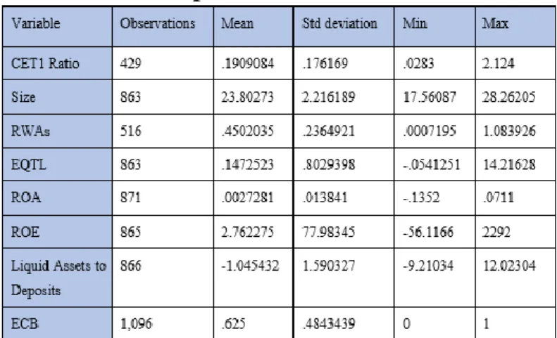
S

After selecting our sample and variables, we treated the chosen variables for our model. In annex, Table VI presents the descriptive statistics, that summarizes the features of our data collection. We can check that our sample has 426 observations of the dependent variable, and that CET1 ratio mean is 19,09%.

The maximum observed for CET1 ratio refers to KOMMUNINVEST I SVERIGE AB in 2017. This company is a Swedish local government funding agency. This observation (212 percent) is justified by the fact that this company’s scheme helps municipal governments to raise capital through the issuance of bonds. On the other hand, the minimum observed value for CET1 ratio is reported by

PANCRETAN COOPERATIVE BANK in 2013. This company is a Greek regional cooperative bank, providing retail banking products and services to local privates, self-employed professionals and SMEs.

Regarding the minimum observed value for size variable reflects INBANK AS’s reported size of 2015. The maximum reflects CREDIT AGRICOLE’s reported size of 2011. INBANK AS was founded in 2015, which can explain the fact that it presents the minimum size of our sample. CREDIT AGRICOLE is one of the biggest banks in Europe, and in 2011 closed several agreements, e.g. the Carispezia acquisition.

Concerning the RWA_TA variable, the minimum value is the percentual reported amount by WELLS FARGO BANK INTERNATIONAL in 2017. The maximum reflects the amount reported by AEGEAN BALTIC BANK, a Greek credit institution, in 2016. The higher the Risk-weighted assets, the higher it will be the minimum amount of capital that must be held in order to reduce the risk of insolvency (Basel Commitee on Banking Supervision, 2011).

The minimum of the variable EQTL reflects CZECH NATIONAL Banks’ bank leverage reported in 2017. The maximum refers to the EUROPEAN STABILITY MECHANISM’s amount in 2014. EUROPEAN STABILITY MECHANISM is an international organisation that provides financial assistance to eurozone members whenever they are in financial difficulty. As referred in the previous section, low leveraged banks result in a higher ratio of EQTL, and high leveraged ones would have a lower EQTL ratio.

For ROA, the minimum value belongs to the 2013 NOVA KREDITNA BANKA MARIBOR D.D. reported amount. The maximum amount reflects the return on assets of INBANK AS in 2017.

The ROE’s minimum and the maximum observed value belong to ARBEJDSMARKEDETS TILLAEGSPENSION in 2018 and 2013, respectively. This is an investor of pension funds in Denmark.

And lastly, the minimum observed for the ratio of the natural logarithm of Liquid assets over short-term deposits refers to the observation of GE CAPITAL

EUROPEAN FUNDING in 2018. This is an Irish company formed with the purpose of issuing debt securities to repay existing credit facilities, refinance indebtedness, and for acquisition purposes. Liquid assets to deposits maximum observed value belongs to WELLS FARGO BANK INTERNATIONAL (Ireland) in 2011.

In annex, Table VII displays the correlation matrix of the variables used in our regression analysis.

Following the previous section, where we put forward our beliefs with respect to the correlation between the dependent and the independent variables, Table VII shows the real correlation between them.

As we can see, the size variable exhibits a negative relationship with the dependent variable. This is in accordance with previous literature (See: Klepczarek, 2015; Ahmad et al., 2008; Bateni et al., 2014).

RWA_TA also has a negative correlation with the dependent variable, meaning

that an increase in RWAs variable will reflect a decrease in CET1 ratio. This responds to our expectations and is also in line with previous literature (Rime, 2001; Bateni et al., 2014).

EQTL variable presents a positive correlation with CET1 ratio, pursuant to what

we expected taking into consideration previous studies on capital ratios (Ahmad et

al., 2008).

It is observed that ROA has a positive correlation with the dependent variable. Although the impact of ROA in the CET1 ratio is not consensual in the literature, our results are in line with Bateni et al. (2014).

ROE in our regression seems to be negatively correlated with CET1 ratio. Past

studies also confirm that ROE shows a negative impact on capital (Asarkaya & Ozcan, 2007; Bateni et al., 2014).

The ratio between Liquid Assets and Deposits presents a positive relationship with CET1 ratio. Which means that when the ratio of Liquid Assets to Deposits increases, CET1 ratio tends to increase. That is aligned with our expectations presented in the previous section (Ahmad et al., 2008).

Regarding our dummy variable ECB, it has a positive impact on CET1 ratio. This means that quantitative easing6 implementation increased CET1 ratio. A decrease of commercial banks’ assets, and therefore, of the denominator of CET1 ratio, which makes the overall ratio to increase (all else being equal).

3.5

R

A

Performing a robustness analysis allows us to check if the results obtained stay the same given a change in inputs. Therefore, we replicate the model observing for the following effects: country, year, firm, random and fixed. Additionally, we correct ROE and CET1 ratio, submitting them to a winsor process.

Winsorizing will allow us to limit extreme values in our data in order to reduce the effect of possible spurious outliers (Rousseeuw & Leroy, 1987). Our data is not normally distributed, and as we know distribution can be heavily influenced by outliers (Mehmetoglu & Jakobsen, 2017). So, applying this transformation we can reduce the possibility of our data to be influenced by outliers. We only applied it to

ROE and CET1 ratio because these variables had more extreme values. Winsorized

estimators are usually more robust than the standard ones. Applying winsorization, our residuals seems to approximate more to a normal distribution, as you can see in kernel density graph (Figure 4 and 5).

Table I exhibits the descriptive statistics taking into consideration the corrections in ROE and CET1 ratio.

6 _{ECB’s measure of buying assets from commercial banks, as part of its monetary policy measures,}

Table I - Descriptive statistics (Robustness check)

Variable Observations Mean Std deviation Min Max

CET1 Ratio_w 429 .184711 .1272641 .055 .8026 Size 863 23.80273 2.216189 17.56087 28.26205 RWA_TA 516 .4502035 .2364921 .0007195 1.083926 EQTL 863 .1472523 .8029398 -.0541251 14.21628 ROA 871 .0027281 .013841 -.1352 .0711 ROE_w 865 .0656516 .2613421 -1.1493 1.3367 LiquidAss_Dep 866 -1.045432 1.590327 -9.21034 12.02304 ECB 1,096 .625 .4843439 0 1

In Table I the variables signalized with “_w” are the ones that were submitted to winsorization.

The correlation between the dependent and independent variables is close to our model with the standard variables (Table VIII).

In addition to winsorization, we also performed different regressions. The objective is to reinforce the conclusions obtained, because findings based on a single method may distort the results. Thus, the application of several methods to address our research question will strengthen the results.

4. R

ESULTS

This chapter exhibit and discuss the results. Section 4.1 displays the results arising from our determinants’ estimation of the CET1 ratio. Section 4.2 presents the robustness analysis results.

4.1

D

CET1

R

What were the determinants of CET1 ratio in European Union banks after the Sovereign Debt Crisis?

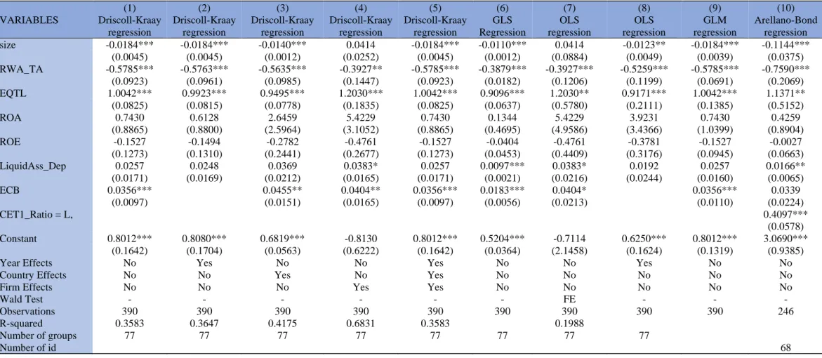
In order to answer our research question, we assess the determinants of the CET1 ratio and present the results in Table II.

As we can observe, with an exception for Model 4 and 7, size presents a significant and negative impact in CET1 ratio. Large banks appear to have a lower CET1 ratio. For the two regressions in Model 4 and 7, size does not impact the CET1 ratio and has a positive coefficient, which is the opposite of what we expected. Larger banks tend to increase their capital ratios more than other banks (Rime, 2001).

In all Models, the RWA_TA is negatively related to CET1 ratio. This was already verified in previous literature (See, for example: Klepczarek, 2015; Brink & Arping, 2009). The correlation between risk and capital is often negative due to the difference in risk perception. The assets that a regulator classifies as a high level of risk are not considered as risky by managers (Wong et al, 2008). Thus, since our Models shows that RWA_TA negatively affects the CET1 ratio, it confirms the difference in risk perception within regulatory authorities and managers.

The results are consistent in all Models regarding EQTL. This variable presents a positive correlation with the CET1 ratio. As seen in previous literature, low leverage banks would have a higher CET1 ratio (Ahmad et al, 2008).

ROA and ROE don’t have a significant impact on CET1 ratio. Nonetheless, their

coefficients sign are in line with previous literature and with our expectations (See Klepczarek, 2015; Bateni et al, 2014).

In relation to the ratio of Liquid assets over deposits, we observe in Models 4, 6, 7 and 10 that it has a significant and positive correlation with the CET1 ratio. As we expected, banks with more liquidity appear to have a higher CET1 ratio (Ahmad

et al, 2008).

The Quantitative Easing effect, that we express by ECB, appears to have a positive and statistical significance in all models except in Model 10. Model 10 represents an Arellano–Bond linear dynamic panel-data estimation, where it is considered the lag effect of the dependent variable. In other words, what happens in the independent variable only impacts the dependent one period after. Therefore, the Quantitative Easing effect of, for example, 2010 do not influence 2011’s CET1 ratio.

Table II - Determinants of CET1 Ratio VARIABLES (1) Driscoll-Kraay regression (2) Driscoll-Kraay regression (3) Driscoll-Kraay regression (4) Driscoll-Kraay regression (5) Driscoll-Kraay regression (6) GLS Regression (7) OLS regression (8) OLS regression (9) GLM regression (10) Arellano-Bond regression size -0.0184*** -0.0184*** -0.0140*** 0.0414 -0.0184*** -0.0110*** 0.0414 -0.0123** -0.0184*** -0.1144*** (0.0045) (0.0045) (0.0012) (0.0252) (0.0045) (0.0012) (0.0884) (0.0049) (0.0039) (0.0375) RWA_TA -0.5785*** -0.5763*** -0.5635*** -0.3927** -0.5785*** -0.3879*** -0.3927*** -0.5259*** -0.5785*** -0.7590*** (0.0923) (0.0961) (0.0985) (0.1447) (0.0923) (0.0182) (0.1206) (0.1199) (0.0691) (0.2069) EQTL 1.0042*** 0.9923*** 0.9495*** 1.2030*** 1.0042*** 0.9096*** 1.2030** 0.9171*** 1.0042*** 1.1371** (0.0825) (0.0815) (0.0778) (0.1835) (0.0825) (0.0637) (0.5780) (0.2111) (0.1385) (0.5152) ROA 0.7430 0.6128 2.6459 5.4229 0.7430 0.1344 5.4229 3.9231 0.7430 0.4259 (0.8865) (0.8800) (2.5964) (3.1052) (0.8865) (0.4695) (4.9586) (3.4366) (1.0399) (0.8904) ROE -0.1527 -0.1494 -0.2782 -0.4761 -0.1527 -0.0404 -0.4761 -0.3781 -0.1527 -0.0027 (0.1273) (0.1310) (0.2441) (0.2677) (0.1273) (0.0453) (0.4409) (0.3176) (0.0945) (0.0663) LiquidAss_Dep 0.0257 0.0248 0.0369 0.0383* 0.0257 0.0097*** 0.0383* 0.0192 0.0257 0.0166** (0.0171) (0.0169) (0.0212) (0.0165) (0.0171) (0.0021) (0.0216) (0.0244) (0.0160) (0.0065) ECB 0.0356*** 0.0455** 0.0404** 0.0356*** 0.0183*** 0.0404* 0.0356*** 0.0339 (0.0097) (0.0151) (0.0165) (0.0097) (0.0056) (0.0213) (0.0110) (0.0224) CET1_Ratio = L, 0.4097*** (0.0578) Constant 0.8012*** 0.8080*** 0.6819*** -0.8130 0.8012*** 0.5204*** -0.7114 0.6250*** 0.8012*** 3.0690*** (0.1642) (0.1704) (0.0563) (0.6222) (0.1642) (0.0364) (2.1458) (0.1624) (0.1319) (0.9385)

Year Effects No Yes No No Yes No No Yes No No

Country Effects No No Yes No Yes No No No No No

Firm Effects No No No Yes Yes No No No No No

Wald Test - - - FE - - -

Observations 390 390 390 390 390 390 390 390 390 246

R-squared 0.3583 0.3647 0.4175 0.6831 0.3583 0.1988

Number of groups 77 77 77 77 77 77 77 77

Number of id 68

Note: This table presents the results of the determinants of CET1 Ratio. Model 1 refers to a regression with Driscoll-Kraay standard errors. Model 2 is a regression with Driscoll-Kraay standard errors with year effects, while Model 3 is with country effects, Model 4 with firm effects, and Model 5 with year, country and firm effects. Model 6 is based on a GLS regression. Model 7 and 8 are OLS regressions with fixed effects and year effects, respectively. Mo del 9 is a generalised linear model. Model 10 is an Arellano–Bond linear dynamic panel-data estimation. Robust standard errors in parentheses. OLS= ordinary least squares; GLM= generalized linear

4.2

R

A

R

Table III exposes the results obtained replicating the models used and applying a winsorized process to CET1 ratio and ROE. We decide to do this transformation in these two variables given their discrepancy of minimum and maximum values. Despite these values were justified by the nature business of the entities that have such values, they are far from what is normal in our sample. Thus, we applied the winsorized process to these variables, in order to limit extreme values (Rousseeuw & Leroy, 1987). The robustness analysis strengthens the results that we came with. Results achieved with such transformations are similar to the results presented previously.

Size has a significant and negative correlation with CET1 ratio in all Models,

except for Model 4 and 7, just like it had without winsorizing ROE and CET1 ratio. The difference is that with this transformation, in model 4 and 7 the coefficient is negative.

The results in RWA_TA, EQTL and ROA are consistent since they are the same with and without winsorizing. RWA_TA is significant and influences negatively the CET1 ratio. EQTL also remains significant and positively impacts the CET1 ratio. While ROA still has a positive coefficient but doesn’t impact the CET1 ratio.

ROE, which was submitted to winsorization, is now significant in Models 6 and

9. Meaning that in Models 6 and 9 ROE does have a significant and negative impact in CET1 ratio. Regarding the rest of the Models, the results are consistent with the ones reported before.

Regarding the ratio between Liquid assets and deposits, the results are similar. In this hypothesis, it is significant and has a positive impact on the dependent variable in Model 3, in addition to Models 4, 5, 6, 7 and 10. Thus, it appears that now, LiquidAss_Dep has a positive and significant relationship with the CET1 ratio taking into consideration country effects.

Table III - Determinants of CET1 Ratio (Winsorized) VARIABLES (1) Driscoll-Kraay regression (2) Driscoll-Kraay regression (3) Driscoll-Kray regression (4) Driscoll-Kraay regression (5) Driscoll-Kraay regression (6) GLS regression (7) OLS regression (8) OLS regression (9) GLM regression (10) Arellano-Bond regression Size -0.0149*** -0.0149*** -0.0186*** -0.0079 -0.0172 -0.0109*** -0.0079 -0.0096* -0.0149*** -0.0886*** (0.0021) (0.0021) (0.0024) (0.0138) (0.0174) (0.0009) (0.0480) (0.0050) (0.0025) (0.0315) RWA_TA -0.5340*** -0.5330*** -0.5106*** -0.4101*** -0.3905*** -0.4092*** -0.4101*** -0.4264*** -0.5340*** -0.6105*** (0.0689) (0.0713) (0.0734) (0.1030) _(0.0990) (0.0148) (0.1014) (0.0831) (0.0551) (0.1156) EQTL 1.0327*** 1.0254*** 0.9385*** 0.9370*** 0.8185*** 0.9364*** 0.9370** 0.8526*** 1.0327*** 0.8342*** (0.0594) (0.0605) (0.0724) (0.1032) (0.1019) (0.0526) (0.3735) (0.2624) (0.1327) (0.2188) ROA 0.6166 0.5821 1.2972 1.7317 1.7004 0.2749 1.7317 1.7528 0.6166 0.1982 (0.7550) (0.7454) (1.7146) (1.1137) (1.0973) (0.3638) (1.6966) (1.5708) (0.7680) (0.4922) ROE_w -0.1311 -0.1327 -0.1650 -0.1709 -0.1713 -0.0613* -0.1709 -0.1814 -0.1311* -0.0078 (0.1058) (0.1081) (0.1757) (0.0977) (0.0992) (0.0369) (0.1768) (0.1638) (0.0770) (0.0524) LiquidAss_Dep 0.0094 0.0090 0.0159* 0.0230** 0.0185* 0.0041*** 0.0230** 0.0101 0.0094 0.0163*** (0.0067) (0.0065) (0.0082) (0.0079) (0.0081) (0.0014) (0.0114) (0.0118) (0.0081) (0.0063) ECB 0.0279*** 0.0315*** 0.0281** 0.0188*** 0.0156*** 0.0281** 0.0279*** 0.0240** (0.0063) (0.0078) (0.0101) (0.0037) (0.0041) (0.0123) (0.0080) (0.0110) CET1_Ratio_w = L, 0.3501** (0.1455) Constant 0.6743*** 0.6798*** 0.7489*** 0.4181 0.6924 0.5211*** 0.4786 0.5087*** 0.6743*** 2.4304*** (0.0771) (0.0808) (0.0876) (0.3387) (0.4769) (0.0280) (1.1726) (0.1401) (0.0777) (0.7881)

Year Effects No Yes No No Yes No No Yes No No

Country Effects No No Yes No Yes No No No No No

Firm Effects No No No Yes Yes No No No No No

Wald Test - - - FE - - -

Observations 390 390 390 390 390 390 390 390 390 246

R-squared 0.5025 0.5070 0.5651 0.8690 0.8726 0.3579

Number of groups 77 77 77 77 77 77 77 77

Number of id 68

Note: This table presents the results of the determinants of CET1 Ratio. Model 1 refers to a regression with Driscoll-Kraay standard errors. Model 2 is a regression with Driscoll-Kraay standard errors with year effects, while Model 3 is with country effects, Model 4 with firm effects, and Model 5 with year, country and firm effects. Model 6 is based on a GLS regression. Model 7 and 8 are OLS regressions with fixed effects and year effects, respectively. Mo del 9 is a generalised linear model.

In Table III we observe that ECB is positive and statistically significant in every Model. With the winsorization process, the effect caused by the Quantitative Easing in period 0 will affect the CET1 ratio in period 1.

The robust analysis results confirm the results and strengthen the conclusions reached.

5. C

ONCLUSION

This work aims to identify the determinants of the CET1 ratio of European banks between 2011 and 2018. Our results are mainly aligned with existing literature.

We found that larger banks have lower CET1 ratio. This is in line with the “Too big to fail” doctrine. Larger banks feel safer, so they don’t feel the need to have capital buffers (Klepczarek, 2015).

Riskier banks have a lower CET1 ratio (Das & Ghosh, 2004; Asarkaya & Ozcan, 2007). This can be justified by looking at the formulas of both ratios. The ratio to measure risk is calculated as RWAs over Total Assets, and the CET1 ratio is calculated as CET1 capital over RWA. Increasing the RWAs, and consequently the banks’ risk, we are simultaneously decreasing the CET1 ratio. In our study, we verified that variable RWA_TA negatively correlates with the CET1 ratio.

We have evidence to conclude that banks with a lower ratio of total equity to liabilities have a lower CET1 ratio. High leverage banks would hold less equity since they face difficulties in raising equity, so their CET1 ratio would be lower (Ahmad et al., 2008).

We also found that banks with more liquidity are more solvents. Liquidity has a positive impact on banks’ capital ratios (Angbazo, 1997; Ahmad et al., 2008). Higher liquid banks have an easier ability to transfer hard assets into cash, so they have more ease to money assess. In case of a crisis they would be in advance.

Additionally, the measure held by ECB to purchase financial assets appears to increase the banks’ capacity to absorb potential losses, since it has a positive impact in CET1 ratio.

The present paper contributes to the already existing literature. Nonetheless, further research on this topic needs to be undertaken, given the subject’s importance.

Our study limitation regards mainly the data used. Due to unavailable data we could not use a larger period, which would be much more interesting. We had constraints in the period used and the data available by bank. With a larger period, we could address better the Sovereign Debt Crisis effects. Results would have been more robust if we had the same data available for all the banks in our sample. We did not have the same number of observations by banks. If we had used only quoted banks in our study, we might not have such problems, but by doing that selection, we would be biased our sample. Choosing only quoted banks would result in a sample composed only by banks with the greatest importance in the financial system.

Future researchers should use larger samples to robust their results, in order to overcome the problem of unavailable data. It would also be interesting to use a wider timeframe. This will only be possible when there is a database with extensive financial information about all banks, and not only about the quoted ones.

R

EFERENCES

Acharya, V., Drechsler, I. and Schnabl, P. (2014b) ‘A Pyrrhic Victory? Bank Bailouts and Sovereign Credit Risk’, Journal of Finance, 69(6), pp. 2689–2739. Acharya, V. V. et al. (2018) ‘Real effects of the sovereign debt crisis in Europe: Evidence from syndicated loans’, Review of Financial Studies, 31(8), pp. 2855– Acharya, V. V. and Schnabl, P. (2010) ‘Do global banks spread global imbalances? Asset-backed commercial paper during the financial crisis of 2007-09’, IMF

Economic Review. Palgrave Macmillan, 58(1), pp. 37–73.

Ahmad, R., Ariff, M. and Skully, M. J. (2008) ‘The determinants of bank capital ratios in a developing economy’, Asia-Pacific Financial Markets, 15(3–4), pp. 255– 272.

Ali, T. M. (2012) ‘the Impact of the Sovereign Debt Crisis on the Eurozone Countries’, Procedia - Social and Behavioral Sciences, 62, pp. 424–430.

Allegret, J. P., Raymond, H. and Rharrabti, H. (2017) ‘The impact of the European sovereign debt crisis on banks stocks. Some evidence of shift contagion in Europe’,