Portfolio Optimization Methods, Their Application and Evaluation
Tomas Hlavaty
Dissertation submitted as partial requirement for the conferral of Master in Finance
Supervisor:
Prof. Sebestyén Szabolcs, Assistant Professor, ISCTE Business School, Department of Finance
-
Spine
-P
o
rt
fo
li
o
O
p
ti
mi
zat
io
n
Me
th
o
d
s,
T
h
ei
r
A
p
p
li
ca
ti
o
n
an
d
E
v
al
u
at
io
n
To
m
a
s H
la
v
a
ty
A
nt
ó
ni
o
A
ug
u
st
o
da
S
il
v
a
Abstract
The submitted master’s thesis focuses on practical application of quantitative portfolio optimization in various forms. The thesis is organized in two main parts, theoretical and practical.
The theoretical part introduces the underpinnings of portfolio theory. It describes the optimization process, introduces a number of selected optimization methods, and provides an overview of portfolio management. As a whole, it serves as an underlying for the practical part.
The practical part of the thesis is based on an experiment that put multiple quantitative portfolio optimization methods into a contest. Different optimizers were applied to portfolios composed of identical assets, which were subsequently held under different portfolio management styles over a pre-specified period of time. The performance of each portfolio was measured ex-post, adequately evaluated in accord with the criteria of the experiment, and confronted with the others.
The questions that this master’s thesis tried to find answers to were (1) which portfolio optimizer, out of the selected ones, performs the best, and (2) whether it is beneficial to conduct rather an active, or a passive portfolio management.
Keywords: Quantitative Portfolio Management, Optimization, Asset Allocation, Diversification JEL Classification: C610, G110
Resumo
Esta dissertação de mestrado apresenta uma aplicação prática da otimização quantitativa de um portfólio realizada de diversas formas. A tese está organizada em duas partes principais, uma teórica e uma prática.
A parte teórica introduz os fundamentos da teoria de portfólio. Descreve o processo de otimização, apresenta vários métodos de otimização selecionadas e fornece uma visão geral da gestão de portfólios. Como um todo, serve como base para a parte prática.
A parte prática da tese coloca vários métodos de otimização de portfólio quantitativos em competição. Diferentes optimizadores foram aplicados a carteiras compostas por ativos idênticos que foram subsequentemente mantidos sob diferentes estilos de gestão ao longo de um período de tempo pré-especificado. O desempenho de cada carteira foi medido ex-post, adequadamente avaliado de acordo com os critérios deotimização e comparado com as demais carteiras.
As perguntas para as quais esta tese de mestrado tentou encontrar respostas foram (1) qual é o optimizador de portfólio, dentre os selecionados, tem o melhor desempenho e (2) se é benéfico conduzir uma gestão de portfólio muito ativa ou passiva.
Palavras-chave: Gestão Quantitativa de Portfólios, Otimização, Alocação de Ativos,
Diversificação
Acknowledgement
I would like to express my gratitude to professor Sebestyén Szabolcs, PhD for supervision of this master‘s thesis. His valuable advices, suggestions, and patience significantly contributed to successful completion of this work.
I also would like to express my deepest thankfulness to my mother, Ing. Jaroslava Alice Hlavata, for her endless support during my entire studies.
Table of Contents
1. Introduction ... 1
2. Portfolio Theory ... 3
2.1. Time Dimension ... 3
2.2. Risk Dimension ... 5
2.3. Modern Portfolio Theory ... 9
2.4. Efficient Frontier ... 13
3. Return Generating Models ... 16
3.1. Capital Asset Pricing Model ... 16
3.2. Market Model ... 18 4. Portfolio Optimization ... 22 4.1. Mean-Variance Optimization ... 22 4.2. Treynor-Black ... 32 4.3. Black-Litterman ... 34 4.4. Naïve Optimization ... 37 5. Portfolio Performance ... 40 6. Portfolio Management ... 45 7. Practical Experiment ... 49 7.1. Optimal Portfolios ... 51 7.2. Results ... 54 7.3. Discussion ... 64 8. Conclusion ... 67 Bibliography ... 69 Annex ... 71
Table of Figures
Figure 1: Efficient frontier for risky assets ... 15
Figure 2: Different CALs for portfolios composed of risk-free and risky assets ... 16
Figure 3: Optimal portfolios for agents with different risk aversion ... 30
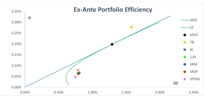
Figure 4: Ex-ante portfolio efficiency... 54
Figure 5: EAR ... 55
Figure 6: Standard deviation ... 56
Figure 7: Residual SD ... 56
Figure 8: Jensen's alpha ... 57
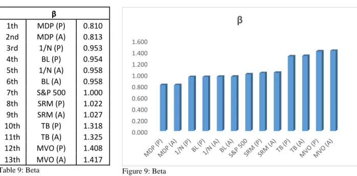
Figure 9: Beta ... 57
Figure 10: Sharpe ratio... 58
Figure 11: Treynor ratio ... 58
Figure 12: Information ratio... 59
Figure 13: M^2... 59
Figure 14: Final ranking... 63
Table of Tables
Table 1: Values of β ... 20
Table 2: Values of A ... 28
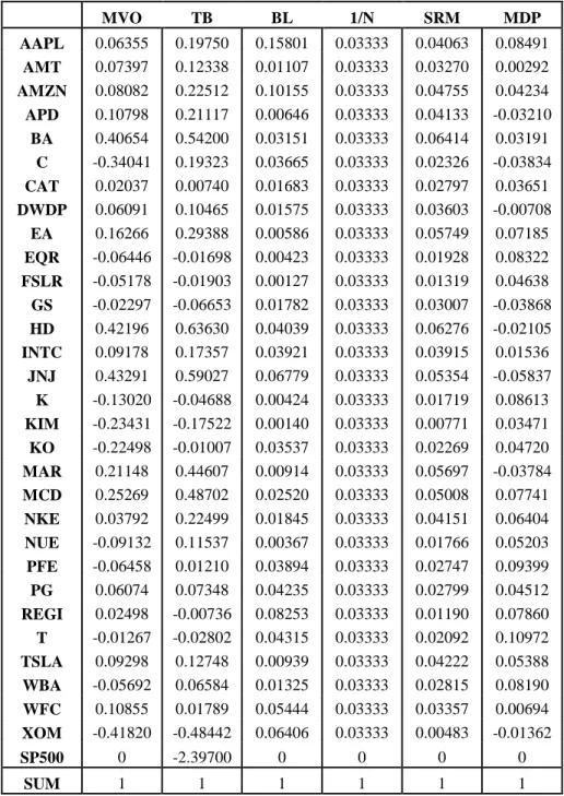
Table 3: Optimal relative asset allocation suggested by the models ... 52
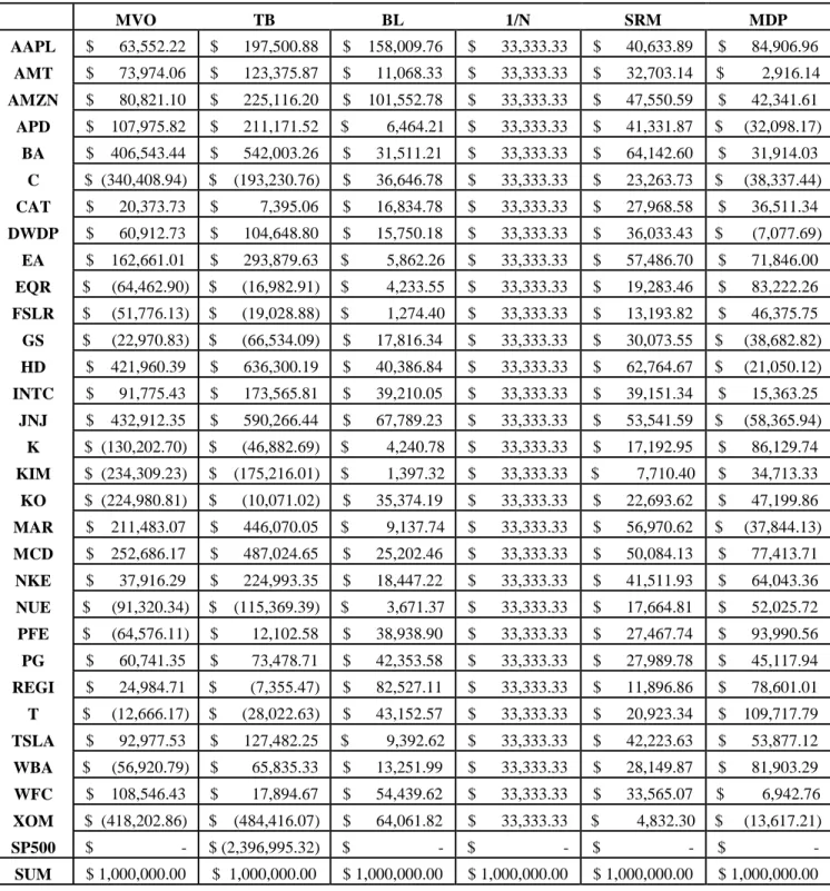
Table 4: Optimal absolute asset allocation suggested by the models ... 53
Table 5: EAR ... 55
Table 6: Standard deviation ... 56
Table 7: Residual SD ... 56
Table 8: Jensen's alpha ... 57
Table 9: Beta ... 57
Table 10: Sharpe ratio ... 58
Table 11: Treynor ratio ... 58
Table 12: Information ratio ... 59
Table 13: M^2 ... 59
Table 14: Portfolio rankings by categories ... 62
Table 15: Final point chart ... 63
Table 16: Final ranking ... 63
1
1. Introduction
“An investment in knowledge pays the best interest”. A famous quote pronounced by
Benjamin Franklin, an American polymath and one of The Founding Fathers of the United States, is pointing clearly to where every person should invest in the first place. Learning is a never-ending process and shall we look at the profiles of the greatest from the greatest, regardless the field of interest, they have never considered their education as complete. The more we invest into our mind, the higher the return we may expect to come back to us in the future in various forms. Our knowing can be seen as a portfolio of knowledge. Portfolio, which we build in more or less constructive matter.
Our knowing deeply influences the way we approach, understand, handle, and reflect all of the challenges we encounter. Based on our obtained experience and our knowing, we derive theories and philosophies. The investment philosophy has alike origin and, as well as other philosophies, is a subject of evolution. Swensen (2000) describes the investment philosophy as a coherent approach being applied consistently to all aspects of portfolio management process. In his eyes, the philosophical principals represent time-tested insights into investment matters that eventually evolve into lasting professional convictions. The investor’s effort to find the most effective way to generate investment returns emanates from those convictions and fundamental beliefs. The investment returns are seen as a product of three tools of portfolio management: (1) asset allocation, (2) security allocation, and (3) market timing. Sophisticated investor then considers contribution of each of the portfolio management tools to costruct portfolios in a conscious manner.
The core focus of this thesis is on the problematics of the first tool of portfolio management, the asset allocation and the various approaches to it. Asset allocation is often understood as the second step of the investment process with the first one being the determination of investor’s investment objectives, time preferences, and risk profile. Various empirical studies over the time have shown that asset allocation has the biggest influence on an overall portfolio performance. Asset allocation represents spreading the investor’s investment capital across various asset classes such as stocks, bonds, derivatives, properties, commodities, funds, cash etc. in order to achieve a diversified portfolio.
2 The thesis is primarily structured in two main parts, theoretical and practical. The theoretical part introduces the underpinnings of portfolio theory. It describes the optimization process, introduces a number of selected optimization methods, and provides an overview of portfolio management. As a whole, it serves as an underlying for the practical part.
The practical part of the thesis is based on an experiment that puts multiple quantitative portfolio optimization methods into a contest. Different optimizers are applied to portfolios composed of identical assets, which are subsequently held under different portfolio management styles over a pre-specified period of time. The performance of each portfolio is measured ex-post, adequately evaluated in accord with the criteria of the experiment, and confronted with the others.
The questions that this master’s thesis tries to find answers to are (1) which portfolio optimizer, out of the selected ones, performs the best, and (2) whether it is beneficial to conduct rather an active, or a passive portfolio management.
3
2. Portfolio Theory
This chapter introduces the fundamentals of portfolio theory, and describes some of the essentials regarding the portfolio optimization frameworks.
In a wide interpretation, any portfolio can be viewed as a set of various items. Those items are acquired by the portfolio’s owner with accordance to his needs, wants, preferences, predispositions, possibilities, and/or expectations. From the financial perspective, such portfolio is understood as a set of financial assets1. The finance universe has two main underlying dimensions: the time dimension and the risk dimension.
2.1.
Time Dimension
The importance of time in finance is absolutely crucial and is best explained by the concept of the time value of money (TVM). TVM concerns equivalence between cash flows occurring at different times. One dollar today has a higher value than one dollar one year from now. However, the same dollar invested today grows in value over time. Formally, the value of one dollar invested today grows accordingly to its interest rate (i). An interest rate is a rate of return that reflects the relationship between differently dated cash flows. When considering the time dimension, we distinguish between the discrete and the continuous time. Consequently, when considering the interest rates under the time dimension framework, we distinguish between the discrete and the continuous interest rates. Therefore, the TVM allows us to either obtain the future value (compounding) or the present value (discounting).
2.1.1. Discrete Time
The discrete time considers a variable to occur at distinct, separate points in time. For instance, monthly, quarterly, yearly. The discrete interest is then being accrued to the principal2 at
those separate points in time. The discrete interest has characteristics of a discrete random variable. Discrete compounding
- the future value (FV) of $1 invested for n years at the interest rate I compounded once per annum
1 Financial asset – a tangible liquid asset which gets its value from a contractual claim 2 Principal - the amount of money originally invested
4
𝐹𝑉 = (1 + 𝑖)𝑛 (2.1)
- FV of $1 compounded m-times per annum for n years
𝐹𝑉 = (1 + 𝑖 𝑚)
𝑚𝑛 (2.2)
Discrete discounting
- the present value (PV) of a future $1 discounted for n years
𝑃𝑉 = 1
(1 + 𝑖)𝑛 (2.3)
- PV of a future $1 discounted m-times a year
𝑃𝑉 = 1
(1 +𝑚)𝑖 𝑚𝑛 (2.4)
2.1.2. Continuous Time
The continuous time also considers the variable to occur at specific points in time. However, and in contrast to the discrete time, between two points in time there is an infinite number of other points of time and the distance between them is converging to zero. Thus, the continuous time sees the variable to occur continuously. The continuous interest does have characteristics of a continuous random variable.
The effect of continuous time, when m → ∞, on compounding can be expressed formally using limits as following:
lim
𝑚→ ∞(1 +
𝑖 𝑚)
5 Continuous compounding
- FV of $1 continuously compounded for n years
𝐹𝑉 = 𝑒𝑖𝑛 (2.6)
Continuous discounting
- PV of $1 discounted with continuously compounded i
𝑃𝑉 = 𝑒−𝑖𝑛 (2.7)
2.2.
Risk Dimension
The risk dimension relates closely with the time dimension. The time dimension distinguishes, in its fundamental property, between two points in time. For instance, between the presence and the future. The presence is well known. However, the future is, from its very nature, uncertain and thus risky. The riskiness, in such case, is the potential deviation from our expectation about the future. Taking the perspective of an investor, the realized return from his investment at the end of the period may be different from the expected one. Those deviations can be both positive or negative. Logically, only the negative deviations are considered undesirable. The most widespread used measure of riskiness in finance is the square root of variance, the standard deviation (SD). The use of SD is convenient under a number of simplifying assumptions, e.g. normal distribution of returns. Also, SD is preferred over variance due to its equality of units with returns as they both are expressed in percentages. Another risk measures are, for example, beta, semi-variance, value-at-risk (VaR), or expected shortfall (ES)
Having mentioned the term expectation, it is convenient to briefly introduce the concept of utility functions, expected utility criterion, and risk aversion. These play a crucial role in the investment decision making process.
2.2.1. Utility Functions
Utility functions are mathematical representations of investor’s attitudes toward risk and return. It is a function that assigns a utility value to all possible investment outcomes. The utility value measures the degree of individual satisfaction the investor receives from any specific level
6 of wealth (W). Such satisfaction may come from several sources, typically from the additional consumption of goods and/or services that the investor can enjoy after selling the investment portfolio. Some investors, on the other hand, may enjoy the satisfaction derived from excitement of the investing game itself (Esch et al., 2005).
The utility functions in general have four important properties: Utility is increasing and is always positive
Marginal utility is decreasing 𝑢′(𝑊1) < 𝑢′(𝑊
0) 𝑤ℎ𝑒𝑛 𝑊1 > 𝑊0 (2.8)
Utility functions are strictly concave
𝑈′′ < 0 (2.9)
Different investors have different utility functions
A utility function, for a given investor and for a given time, is not unique Examples of the most common utility functions
Log utility 𝑢(𝑊) = ln (𝑊) (2.10) Exponential utility 𝑢(𝑊) = 1 − 𝑒−𝑣𝑊 (2.11) Power utility 𝑢(𝑊) =𝑊 1−𝛾 1 − 𝛾 (2.12) Quadratic utility 𝑢 (𝑊) = 𝑊 − 𝑏 2𝑊 2 𝑏 > 0 (2.13)
Where W represents the investor’s wealth.
Special cases of utility functions incorporating the risk aversion coefficients are introduced in the following Section 2.2.2.
7
2.2.1.
Expected Utility Criterion
The expected utility (EU) criterion provides a framework for when an individual must make a decision under uncertainty. That being not knowing which future outcome, out of a set of possible outcomes, is going to result from a decision made today. In such situation, one will make decision that offers the highest expected utility. Each outcome is assigned a probability of occurrence. Thus, the EU is a probability-weighted average of utilities over all possible outcomes and over a specific period of time. The final decision also depends on one’s risk aversion. To demonstrate a general case, let’s consider a lottery L(x,y,π), where outcome x has a probability of occurrence π and y with (1-π). The expected utility is following:
𝐸[𝑈(𝐿)] = 𝜋𝑢(𝑥) + (1 − 𝜋)𝑢(𝑦) (2.14)
The above equation is referred to as the von Neumann-Morgernstern (VNM) utility function and represents the expected utility criterion. Let’s adjust the VNM with respect to asset returns. Let’s consider an asset A at time 𝑡0 with possible future returns 𝑟1, 𝑟2, … , 𝑟𝑛 and with probabilities of occurrence 𝜋𝑟1, 𝜋𝑟2, … , 𝜋𝑟𝑛 at time 𝑡1, respectively. The expected utility can then be expressed as following:
𝐸[𝑈(𝑟𝐴)] = 𝜋𝑟1𝑢(𝑟1) + 𝜋𝑟2𝑢(𝑟2) + ⋯ + 𝜋𝑥𝑛𝑢(𝑟𝑛) = ∑ 𝜋𝑥𝑖𝑢(𝑟𝑖)
𝑛 𝑖=1
(2.15) The expected utility criterion confirms that the individual is concerned only with the final payoffs and the cumulative probability associated with achieving them (Levy and Post, 2005).
2.2.2. Risk Aversion
An important fundamental property of the risk dimension under the portfolio theory framework is the investor’s relation towards risks. His risk aversion. Every investor is different and has a different perception of risks, or in other words, has a different degree of risk aversion. Naturally, the desire of every investor is the same - to avoid risks, i.e. to smooth their consumption across all states of nature and to avoid variations in the value of their portfolio holdings. The investor is considered to be weakly risk averse when
8 the utility of current wealth is higher or equal than the expected utility of potential wealth from a gamble. Strict risk aversion is represented by strict inequality (Beck, 2017).
The risk aversion is measured by the risk aversion coefficients: Absolute risk aversion coefficient
𝛼 (𝑊) = − 𝑢
′′(𝑊)
𝑢′(𝑊) (2.17)
Relative risk aversion coefficient
𝜌 (𝑊) = 𝑊𝛼(𝑊) = − 𝑊𝑢
′′(𝑊)
𝑢′′(𝑊) (2.18)
Risk tolerance coefficient
𝜏 (𝑊) = 1
𝛼 (𝑊)= −
𝑢′(𝑊)
𝑢′′(𝑊) (2.19)
Utility functions incorporating the risk aversion coefficients: Constant absolute risk aversion (CARA)
- Absolute risk aversion is constant at every wealth level - CARA is a function of exponential utility function
𝑢 (𝑊) = − 𝑒−𝛼𝑊 (2.20)
Constant relative risk aversion (CRRA)
- Relative risk aversion is constant at every wealth level - CRRA is a function of power utility function
𝑢 (𝑊) = 𝑊
1−𝜌
9
2.3.
Modern Portfolio Theory
Modern Portfolio Theory (MPT) is a financial portfolio construction theory developed by professor Harry Max Markowitz (1952), which first introduced in his paper “Portfolio Selection” published by the Journal of Science in 1952, and for which he was awarded the Nobel Memorial Prize in Economic Sciences in 1990.
In Markowitz’s paper, the portfolio selection process is divided in two stages. The first stage begins with observations and ends with some expectations regarding the future performance of observed securities. The second stage begins with those expectations and ends with the choice of final optimal portfolio. In this thesis, only the second stage is presented.
MPT, as well as any other theoretical concept, stands upon a number of underlying assumptions. As such, it provides the groundwork for portfolio composition under the mean-variance framework and for an arbitrary number of risky assets, with or without a risk-free asset.
MPT assumptions:
Markets are perfectly efficient No transaction costs, no taxes Assets are perfectly divisible
Risk-free asset is available to all investors Unlimited long and short positions are allowed Investors are rational and risk averse
Utility function is quadratic
Investors possess homogeneous investment motivation, horizon, and expectation Distribution of returns is Gaussian
Investors are concerned only with asset’s mean and variance Investors desire to maximize their expected utility
10
2.3.1. Canonical Portfolio Problem
When an investor faces a portfolio creation decision he needs to make a choice regarding budgeting the asset allocation. Specifically, how much of his capital is going to be allocated to, and spread across, risky assets and how much to risk-free asset as an alternative to risky assets. The future payoff from risky assets is uncertain. However, the payoff from risk-free asset is always certain. The portfolio problem thus becomes the maximization of the expected payoff. That being done in accord with investor’s utility function.
Canonical portfolio problem is well described by Danthine and Donaldson (2015). Let’s consider a risk-free asset 𝑟𝑓 and a number of risky assets with returns 𝑟1, 𝑟2, … , 𝑟𝑖. Also, a portion of capital 𝑤𝑓 being invested into the risk-free asset and (1 − 𝑤𝑓) = ∑𝑛𝑖=1𝑤𝑖 among n risky assets
with 𝑤𝑖 being the individual weight of each risky asset. 𝑤𝑓+ ∑𝑛𝑖=1𝑤𝑖 = 1.
The maximization problem becomes following: 𝑚𝑎𝑥
(𝑤1, 𝑤2, … , 𝑤𝑛) 𝐸 {𝑢 [𝑤𝑓(1 + 𝑟𝑓) + ∑ 𝑤𝑖(𝑟𝑖−
𝑛 𝑖=1
𝑟𝑓)]} (2.22)
Where the term (𝑟𝑖− 𝑟𝑓) represents the risk premium of each risky asset. It is intuitive to assume that the portion of capital invested in risky assets increases with increasing risk premium and decreases when opposite. This intuition can be formally described via the first-order condition (FOC). Under the risk aversion 𝑈′′() < 0, the FOC of the maximization problem becomes
𝐸 {𝑢′ [𝑤𝑓(1 + 𝑟𝑓) + ∑ 𝑤𝑖(𝑟𝑖 − 𝑛 𝑖=1 𝑟𝑓)] ∑(𝑟𝑖 − 𝑟𝑓) 𝑛 𝑖=1 } = 0 (2.23)
The FOC allows to describe the relationship between the investor’s risk aversion and his portfolio’s consumption via the following theorem, Equations 2.24-26, regarding the problem.
11 For simplification, let’s substitute ∑𝑛𝑖=1𝑤𝑖 = 𝑤𝑟 where 𝑤𝑟 represents the capital allocated to risky assets, and 𝐸(𝑟𝑅) = ∑𝑛𝑖=1𝐸(𝑟𝑖)𝑤𝑖 where 𝐸(𝑟𝑅) is the expected payoff of the risky assets combined. Let’s assume 𝑈′′() < 0 and 𝑈′() > 0.
𝑤𝑟 > 0 ↔ 𝐸(𝑟𝑅) > 𝑟𝑓 (2.24)
𝑤𝑟 = 0 ↔ 𝐸(𝑟𝑅) = 𝑟𝑓 (2.25)
𝑤𝑟 < 0 ↔ 𝐸(𝑟𝑅) < 𝑟𝑓 (2.26)
The theorem states that a risk averse investor is willing to make a risky investment if, and only if, the expected payoff from the risky investment exceeds the risk-free rate. Or in other words, if the odds are favorable and there is a positive remuneration from the additional risk accepted.
2.3.2.
Mean-Variance Criterion
MPT considers mean and variance as sufficient information when making a choice regarding the investment assets. It rests on the presumption that rational investors like the asset’s returns and dislikes the return variance. The mean-variance criterion allows the investor to compare various assets between each other while accounting the mean-variance preferences. Let’s assume assets A and B, with 𝜇𝐴, 𝜎𝐴 and 𝜇𝐵, 𝜎𝐵, respectively.
Portfolio A dominates portfolio B if, and only if, the following conditions are satisfied:
𝜇𝐴 ≥ 𝜇𝐵 and 𝜎𝐴 < 𝜎𝐵
Or equivalently,
𝜇𝐴 > 𝜇𝐵 and 𝜎𝐴 ≤ 𝜎𝐵
The mean-variance utility function describes the risk-return trade-off when reflecting the investor’s degree of risk aversion. The function is based on two pivotal assumptions of MPT, the quadratic utility function and the Gaussian distribution of returns. The quadratic utility is important because it implies mean-variance preferences. The Gaussian distribution is attractive due to its simplicity and properties. When considering only mean and variance, the expected utility has following form:
12 𝐸[𝑈(𝑟)] = 𝑢[𝐸(𝑟)] +1
2𝑢
′′[𝐸(𝑟)]𝑉𝑎𝑟(𝑟) (2.27)
To assure consistency with the risk-aversion assumption, the 𝑢′′must be < 0 and hence the positive sign changes to negative. Considering u to be quadratic in form described by Equation 2.13, setting b = 1, and including the investor’s risk aversion coefficient to reflect his perception of risks, we arrive to the standard mean-variance utility function that can be found across the literature and has following form:
𝑈 = 𝐸(𝑟) −1 2𝐴𝜎
2 (2.28)
Where E(r) is the expected return, 𝜎2 is the variance, and A is investor’s risk aversion coefficient.
13
2.4.
Efficient Frontier
Prior to the introduction of the minimum-variance frontier (MVF) and the efficient frontier (EF), it is convenient to define the portfolio expected return and variance/SD in a matrix form, as they are subsequently used throughout the thesis. Let’s consider a portfolio P of n risky assets, with expected returns 𝑟1, 𝑟2, … , 𝑟𝑛 forming N x 1 vector of returns and portfolio’s assets weights 𝑤1, 𝑤2, … , 𝑤𝑛 forming N x 1 vector of weights. The set of covariances between the assets form the
variance-covariance matrix denoted Σ. Vector of expected returns
𝐸(𝑟) = 𝜇 = [ 𝐸(𝑟)1 𝐸(𝑟)2 ⋮ 𝐸(𝑟)𝑛 ]
Vector of portfolio weights
𝑤 = [ 𝑤1 𝑤2 ⋮ 𝑤𝑛 ] Variance-covariance matrix 𝛴 = [ 𝜎112 ⋯ 𝜎1𝑛 ⋮ ⋱ ⋮ 𝜎𝑛1 ⋯ 𝜎𝑛𝑛2 ] Portfolio expected return
𝐸(𝑟𝑝) = 𝜇𝑝 = 𝑤𝑇𝜇 (2.29)
Portfolio variance and SD
𝑉𝑎𝑟(𝑃) = 𝜎𝑃2 = 𝑤𝑇𝛴𝑤 (2.30)
𝑆𝐷 = 𝜎𝑃 = √𝑤𝑇𝛴𝑤 (2.31)
Where the subscript T stands for transposed.
The essential notations being introduced, it is now possible to procced to the introduction of both frontiers. Let’s consider a set of 𝑛 ≥ 2 assets. An infinite number of portfolios can be formed from such set of assets. This creates a set of feasible portfolios, the feasible set. To evaluate efficiency and compare the portfolios, an investor considers their expected returns and variances
14 with accordance to the mean-variance criterion. The investor will choose his or her optimal portfolio from the feasible set, that
1. Offers highest expected return for varying levels of risk, and 2. Offers lowest level of risk for varying levels of expected returns
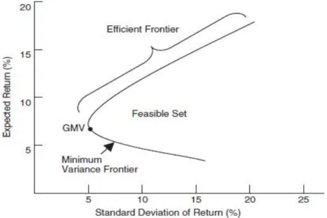
The above-mentioned conditions are known as the efficient set theorem (Sharpe, 1995). The set of portfolios meeting the efficient set theorem are called the efficient portfolios and graphically they plot the EF, which is part of the MVF. EF is the set of frontier portfolios where each portfolio represents the portfolio with the highest expected return for varying levels of risk. Both frontiers are conventionally plotted in an expected return-risk (μ-σ) space. The shape of EF depends whether a risk-free asset is present or not.
2.4.1. Efficient Frontier for Risky Assets
Considering only the risky assets, the graphical representation of MVF and EF is nearly identical yet it is important to distinguish between them. MVF represents the entire curve, EF represents only the non-dominated part of MVF, originating in the global minimum-variance portfolio (GMV). GMV is frontier portfolio with the smallest variance. The shape of MVF is strongly influenced by the correlation (ρ) between the assets as it directly affects the portfolio standard deviation (SD) as descripted by Equation 2.32 for two risky assets A and B, with 𝜇𝐴, 𝜎𝐴
and 𝜇𝐵, 𝜎𝐵, respectively.
𝜎𝑃 = √𝑤𝐴2𝜎𝐴2+ 𝑤𝐵2𝜎𝐵2+ 2𝑤𝐴𝑤𝐵𝜎𝐴𝜎𝐵𝜌𝐴,𝐵 < 𝑤𝐴𝜎𝐴+ 𝑤𝐵𝜎𝐵 (2.32)
The above-mentioned inequality descripts the gain from diversification3 coming from assets with imperfect correlation. Simply put, the lower the correlation between assets, the better the diversification effect, the more parabolic the shape of MVF. The MVF and EF are depicted on the following Figure 1.
15 Figure 1: Efficient frontier for risky assets
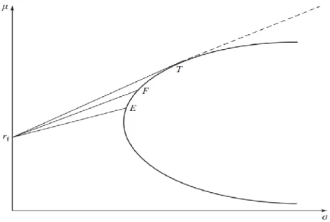
2.4.2. Efficient Frontier for Risk-Free and Risky Assets
The portfolio of assets where one is risk-free affects the shape of EF. Let’s consider two assets, one risky asset A and one risk-free asset, forming a portfolio P. Since the risk-free asset carries no risk, its SD = 0. The SD of such complete portfolio is simply a linear weighted average 𝑆𝐷𝑃 = 𝑤𝐴𝜎𝐴 + 𝑤𝑟𝑓𝜎𝑟𝑓= 𝑤𝐴𝜎𝐴+ 0 where 𝑤𝐴+ 𝑤𝑟𝑓= 1. If short positions on risk-free asset are
allowed, then 𝑤𝐴 > 1 𝑎𝑛𝑑 𝑤𝑟𝑓< 0. The efficient frontier of such combined portfolios is a straight
line originating in the risk-free rate on axis y.
The EF for a combination of n risky assets and a risk-free asset follows the above-described scenario. The risky assets themselves form a parabolic-shaped MVF. The combination of risky portfolio, originally depicted on MVF, with a risk-free asset forms a straight line, referred to as the capital allocation line (CAL) The only CAL that dominates the parabolic curve in all of its length, as well as the other CALs, is the tangent to the MVF. This tangent CAL represents the efficient frontier as depicted in Figure 2. The tangent point represents the only portfolio which can be made solely of risky assets, usually called the tangency portfolio (T). The tangency portfolio is important and plays a crucial role in the investor’s optimal portfolio choice decision process, described in Section 4.1.3.
16 Figure 2: Different CALs for portfolios composed of risk-free and risky assets
3. Return Generating Models
Although asset pricing is not the main subject of interest of this thesis, there are two pricing models that can be considered as essential to the portfolio theory and thus it is convenient for these to be briefly introduced. These models are the capital asset pricing model and the market model. These models represent an alternative to the historical approach when estimating asset’s expected returns, variances, and covariances.
3.1.
Capital Asset Pricing Model
Capital asset pricing model (CAPM) is an equilibrium pricing model and it has played a pivotal role in the development of quantitative investment management since its introduction. CAPM is derived from MPT and as such shares most of the MPT’s assumptions introduced in Section 2.3 with few specifics. As the concept of CAPM is based on the principle of equilibrium, few of the assumptions are worthwhile to review.
17
CAPM assumptions4
All investors have homogeneous expectations regarding returns, variances, and covariances for all assets
Risk-free asset is available for an infinite lending or borrowing Markets are perfectly efficient
All assets are tradable and infinitely divisible Unlimited short sales are allowed
Perfect competition, i.e. an individual alone cannot affect the price Few implications coming from the CAPM assumptions
MVF is identical for all investors EF is identical for all investors as well
As all investors share homogeneous expectations, they all demand the same assets Hence, the tangency portfolio is identical for everyone
Tangency portfolio becomes the market portfolio
According to Litterman (2003), CAPM describes the market equilibrium in a sense that, if the model is correct and any asset’s expected return differs from its equilibrium return, the market forces come into play and restore the relationship suggested by the model. However, CAPM theory goes bit further. As known, risk of a stock can be split between systematic and non-systematic, or specific, risk. If portfolio is large enough, the non-systematic risk can be diversified away5. Since every investor holds a combination of market portfolio and risk-free asset, which both theoretically carry zero of specific risk, the specific risk no longer matters. Therefore, CAPM fundamentally describes a relationship of any asset’s equilibrium return as a linear function of its systematic risk, measured by β, market risk premium and a risk-free rate. The β of market portfolio is always equal to 1. When an asset carries higher systematic risk than the market, i.e. 𝛽 > 1, it should be remunerated by higher return. If the asset carries no systematic risk, thus no specific risk as well, then the equilibrium return should be equal to the risk-free rate. Let’s consider an asset A with
4 Complete list of assumptions is in Section 2.3 5 See Section 3.2.1.
18 return 𝑟𝐴, a risk-free asset with return 𝑟𝑓, and a market portfolio M with return 𝑟𝑀. CAPM
equation is following:
𝑟𝐴 = 𝑟𝑓+ 𝛽𝐴(𝑟𝑀− 𝑟𝑓) (3.1)
Equivalently, let’s substitute the single asset A with a complete portfolio P, then the equation becomes
𝑟𝑃 = 𝑟𝑓+ 𝛽𝑃(𝑟𝑀− 𝑟𝑓) (3.2) This is the standard CAPM, where β is the systematic risk measure of an asset/portfolio, and the term (𝑟𝑀− 𝑟𝑓) is the market risk premium.
The graphical representation of CAPM is the security market line (SML). In CAPM world, all portfolios should lie on SML. SML is plotted in the μ-σ space, originating at the risk-free rate on axis Y and going through the market portfolio M. SML is a useful tool for determining whether an asset is overvalued, undervalued, or correctly valued on the market. This can be done mathematically by comparing the equilibrium return suggested by CAPM and the actual return observed on the market, or graphically plotting the asset’s return together with the SML in one graph.
3.2.
Market Model
Market model belongs to the group of so-called factor models. Factor models represent the building stone of the Arbitrage Pricing Theory (APT), introduced by Ross (1976). The theory is based on an assumption that all asset returns can be determined by a set of factors. It believes that the asset returns are related to each other through their correlations with a limited set of factors. The simplest factor model is the market model. More advanced are, for example, the 3-factor and 5-factor Fama-French models.
The market model (MM) is a one factor model. The factor is the return on market portfolio. MM describes a relationship between the returns on asset and the returns on market portfolio through a classical regression. Let’s assume an asset A with return 𝑟𝐴, and the market portfolio M with return 𝑟𝑀. MM regression equation is following (DeFusco et al., 2007):
19
𝑟𝐴 = 𝛼𝐴+ 𝛽𝐴𝑟𝑀+ 𝜀𝐴 (3.3)
Where 𝛼𝐴 is the intercept representing an average return on asset A independent of the market, and 𝜀𝐴 is the error term representing the residual risk. Alternatively, the MM equation can be expressed in terms of excess returns as following:
𝑟𝐴− 𝑟𝑓 = 𝛼𝐴 + 𝛽𝐴(𝑟𝑀− 𝑟𝑓) + 𝜀𝐴 (3.4)
MM stands upon following assumptions 𝐸(𝜀𝐴) = 0
𝐶𝑜𝑣(𝑟𝑀, 𝜀𝐴) = 0
𝐶𝑜𝑣(𝜀𝐴, 𝜀𝐵) = 0 𝐴 ≠ 𝐵
These assumptions partially correspond to the OLS regression model. However, MM does not assume the error term to be normally distributed, as well as the variance of error term being identical across assets. Given these assumptions, three postulates can be made regarding the expected returns, variances, and covariances.
Expected return of asset A depends on the expected return of market M, A’s β towards M, and the independent part of A’s return
𝐸(𝑟𝐴) = 𝛼𝐴+ 𝛽𝐴𝐸(𝑟𝑀) (3.5) Variance of asset A depends on the variance of market M, the residual variance of A, and
A’s β towards M
𝑉𝑎𝑟(𝑟𝐴) = 𝛽𝐴2𝜎𝑀2 + 𝜎𝜀𝐴
2 (3.6)
Covariance between the returns of asset A and asset B depends on the variance of returns of market M, and A’s and B’s sensitivities 𝛽𝐴, 𝛽𝐵
20
3.2.1. Diversification
The market model is helpful in explanation of one of the core features of large financial portfolios and that being the diversification effect. The positive effect of correlation on diversification is introduced already in Section 2.4.1. In this section, the concept of diversification is extended with regard to the number of assets within the portfolio.
Let’s assume an asset, e.g. a stock. Each stock’s total risk is primarily composed of two main types of risk. The systematic risk and the specific risk.
Systematic risk, or market risk, refers to the risks associated with the macroeconomic events or developments impacting the entire market. Market risk impacts all market participants equally and from its nature cannot be eliminated via diversification. However, its impacts can be eased using an appropriate hedging or asset allocation strategy. Systematic risk is measured by β. Beta of an asset can be interpreted as its sensitivity towards the market. Beta of the market is always equal to 1. Let’s assume an asset A and a market portfolio M, with returns 𝑟𝐴 and 𝑟𝑀, respectively. β calculation is following:
𝛽𝐴 =
𝑐𝑜𝑣(𝑟𝐴, 𝑟𝑀)
𝑣𝑎𝑟(𝑟𝑀) (3.8)
Beta of a portfolio is calculated as a weighted average of individual asset betas. Let’s assume a portfolio P with n assets. β calculation is following:
𝛽𝑃 = ∑ 𝑤𝑖𝛽𝑖
𝑛 𝑖=1
(3.9)
β < 0 Asset returns move the opposite direction compared to the market. If the market return is positive, the asset return is negative and vice versa.
β = 1 Asset returns move identically with the market.
β > 1 Asset returns move the same direction as the market but quicker, both up and down. The asset is riskier than the market.
0 < β < 1 Asset returns move the same direction as the market but slower, both up and down. The asset is less risky than the market.
21 Specific risk, or idiosyncratic risk or residual risk, refers to the risks associated with an
individual industry, firm, or product. Specific risk can be eliminated via diversification. The elimination of specific risk from a portfolio is a sought-after benefit. Mathematically, the elimination can be explained by using the properties of the market model. Let’s consider the MM’s second postulate for an entire portfolio P consisting of n assets as following (Elton et al., 2011):
𝑉𝑎𝑟(𝑟𝑝) = 𝛽𝑃2𝜎𝑀2 + 𝜎𝜀2𝑃 (3.10) Where the term 𝑉𝑎𝑟(𝑟𝑝) represents the total risk, 𝛽𝑃2𝜎𝑀2 the systematic risk, and 𝜎𝜀𝑃
2 the
specific risk. In terms of n individual assets, the equation can be re-written as following:
𝑉𝑎𝑟(𝑟𝑝) = 𝛽𝑃2𝜎𝑀2 + 𝜎𝜀2𝑃 = ∑ 𝑤 𝑖2𝛽𝑖2𝜎𝑀2 + ∑ 𝑤𝑖2𝜎𝜀𝑖 2 𝑛 𝑖=1 𝑛 𝑖=1 (3.11) For evidential purposes, it is convenient to ignore the systematic risk part and focus solely on the specific one. Moreover, let’s assume an equally weighted portfolio where 𝑤𝑖 = 1
𝑛 , the
diversification effect on the specific part is following:
∑ 𝑤𝑖2𝜎𝜀2𝑖 𝑛 𝑖=1 = ∑ (1 𝑛) 2 𝜎𝜀2𝑖 𝑛 𝑖=1 = 1 𝑛2∑ 𝜎𝜀𝑖 2 𝑛 𝑖=1 = lim 𝑛→∞ ∑𝑛𝑖=1𝜎𝜀2𝑖 𝑛2 = 0 (3.12)
It is easy to see that with a number of assets increasing to infinity, the specific risk converges towards zero.
22
4. Portfolio Optimization
Since the introduction of MPT in 1952, a number of portfolio optimization techniques have been developed. All of them, however, more or less build upon the mean-variance optimization (MVO) model with the motivation to overcome some of its main drawbacks. The time has proven that the MVO developed by professor Harry Markowitz has truly become the cornerstone of the portfolio theory. This chapter regarding portfolio optimization introduces only the methods used in the practical part of this thesis.
4.1.
Mean-Variance Optimization
This section dedicated to the MVO is a direct continuation of Section 2.4 regarding the efficient frontier. As introduced there, the EF is influenced by the parameters of individual assets. Their means, variances, covariances, and the presence of risk-free asset.
4.1.1. MVO for Risky Assets
To compute portfolios making up the EF considering only the risky assets, the following constrained problem must be satisfied
𝑚𝑖𝑛 𝑤𝑇𝛴𝑤 𝑠. 𝑡. 𝑤𝑇𝜇 = 𝑟𝑅
𝑤𝑇𝐼 = 1
Where I is the N x 1 column vector of ones, and 𝑟𝑅 is the required portfolio return6 demanded by the investor. No non-negativity constrains are present. The problem can be solved by minimizing the Lagrangian
min ℒ =1 2𝑤
𝑇𝛴𝑤 + 𝜆(𝑟
𝑅 − 𝑤𝑇𝜇) + 𝛾(1 − 𝑤𝑇𝐼) (4.1)
6 The use of required return is convenient as the investor may desire a return different from the expected return.
Nonetheless, the expected return may be used in the computations as well. Required return is often referred to as target return.
23 Where 𝜆 and 𝛾 are the Lagrange multipliers. The first-order conditions to solve the Lagrangian are following:
𝜕ℒ 𝜕𝑤 = 𝛴𝑤 − 𝜆𝜇 − 𝛾𝐼 = 0 (4.2) 𝜕ℒ 𝜕𝜆 = 𝑟𝑅 − 𝑤 𝑇𝜇 = 0 (4.3) 𝜕ℒ 𝜕𝛾 = 1 − 𝑤 𝑇𝐼 = 0 (4.4)
The FOCs with applied constrains can be re-written in terms of portfolio weights as following:
𝑤 = 𝑤𝑃 = 𝜆𝛴−1𝜇 + 𝛾𝛴−1𝐼 (4.5)
𝑟𝑅 = 𝑤𝑇𝜇 = 𝜇𝑇𝑤 = 𝜆(𝜇𝑇𝛴−1𝜇) + 𝛾(𝜇𝑇𝛴−1𝐼) (4.6) 1 = 𝐼𝑇𝑤
𝑃 = 𝑤𝑃𝑇𝐼 = 𝜆(𝐼𝑇𝛴−1𝜇) + 𝛾(𝐼𝑇𝛴−1𝐼) (4.7)
For simplification purposes, Danthine and Donaldson (2015) use the following constants 𝐴 = 𝐼𝑇𝛴−1𝜇 = 𝜇𝑇𝛴−1𝐼 (4.8)
𝐵 = 𝜇𝑇𝛴−1𝜇 > 0 (4.9)
𝐶 = 𝐼𝑇𝛴−1𝐼 > 0 (4.10)
𝐷 = 𝐵𝐶 − 𝐴2 > 0 (4.11)
Solving the set of FOCs, with applied substitution, for the Lagrange multipliers, we obtain:
𝜆 =𝐶𝑟𝑅− 𝐴
𝐷 𝑎𝑛𝑑 𝛾 =
𝐵 − 𝐴𝑟𝑅 𝐷
Finally, substituting for the Lagrange multipliers into the Equation 4.5, the solution for portfolio weights is following:
𝑤𝑃 = 𝐶𝑟𝑅− 𝐴
𝐷 𝛴
−1𝜇 + 𝐵 − 𝐴𝑟𝑅
𝐷 𝛴
24 Re-arranging the terms, the solution can be written in an alternative form as following:
𝑤𝑃 = 1 𝐷[𝐵(𝛴 −1𝐼) − 𝐴(𝛴−1𝜇)] + 1 𝐷[𝐶(𝛴 −1𝜇) − 𝐴(𝛴−1𝐼)]𝑟 𝑅 (4.13) Or, 𝑤𝑃 = 𝑔 + ℎ𝑟𝑅 (4.14)
Where g represents the weight vector for portfolio with 𝑟𝑅 = 0 , and g + h represents the weight vector for portfolio with 𝑟𝑅 = 1
The FOCs are essential in defining the portfolio weights representing any frontier portfolio for a given level of required return. The solution for portfolio weights is highly practical as it delivers the weights of corresponding frontier portfolio for a chosen level of desired return.
The computation of parameters of any frontier portfolio is quite a straightforward matter. Expected return
𝐸(𝑟𝑃) = 𝜇𝑃 = 𝑤𝑃𝑇𝜇 (4.15)
Where 𝑤𝑃 is the portfolio weights, and 𝜇 is vector of expected returns of assets. Variance 𝑉𝑎𝑟(𝑃) = 𝜎𝑃2 = 𝑤 𝑃𝑇𝛴𝑤𝑃 = 𝐶 𝐷(𝜇𝑃− 𝐴 𝐶) 2 +𝐴 𝐶 (4.16)
The global minimum-variance portfolio (GMV), is the frontier portfolio with the smallest variance. It represents a pivotal point on the MVF, as it splits the MVF between the efficient and non-efficient frontier. The portfolio parameters calculated by Equations 2.29-31 apply for GMV as well. However, it can be calculated in a simpler way:
25 Expected return 𝐸(𝑟𝑔𝑚𝑣) = 𝜇𝑔𝑚𝑣 = 𝐴 𝐶 (4.17) Variance 𝑉𝑎𝑟(𝑔𝑚𝑣) = 𝜎𝑔𝑚𝑣2 = 1 𝐶 (4.18)
4.1.2. MVO for Risk-free and Risky Assets
The inclusion of a risk-free asset within a portfolio of otherwise risky assets improves the efficiency of the complete portfolio. Let’s assume a fraction of capital denoted w invested in a vector of risky assets and (1 − 𝐼𝑇𝑤) in the risk-free asset denoted 𝑤
𝑓. The optimization problem
is following:
𝑚𝑖𝑛 𝑤𝑇𝛴𝑤 𝑠. 𝑡. 𝑟𝑓+ (𝜇 − 𝑟𝑓𝐼)
𝑇
𝑤 = 𝑟𝑅
Where μ represents the vector of expected returns on risky assets, 𝑟𝑓 the return on risk-free
asset, and I the vector of ones.
It is worthwhile to mention that the constrain 𝑤𝑇𝐼 = 1 is no longer present. Thus, 𝑤𝑓+
∑𝑛𝑖=1𝑤𝑖 ≠ 1. No non-negativity constrains are present. The problem can be solved by minimizing
the Lagrangian:
min ℒ =1 2𝑤
𝑇𝛴𝑤 + 𝜆(𝑟
𝑅 − 𝑟𝑓− (𝜇 − 𝑟𝑓𝐼)𝑇𝑤 (4.19)
Where 𝜆 is the Lagrange multiplier. The FOCs to solve the Lagrangian are following: 𝜕ℒ 𝜕𝑤= 𝛴𝑤 − 𝜆(𝜇 − 𝑟𝑓𝐼) = 0 (4.20) 𝜕ℒ 𝜕𝜆 = 𝑟𝑅 − 𝑟𝑓− (𝜇 − 𝑟𝑓𝐼) 𝑇 𝑤 = 0 (4.21)
26 The FOCs can be re-written in terms of portfolio weights as following:
𝑤 = 𝜆𝛴−1(𝜇 − 𝑟𝑓𝐼) (4.22)
𝑤 = 𝑟𝑅 − 𝑟𝑓
(𝜇 − 𝑟𝑓𝐼)𝑇 (4.23)
Applying the constrain and solving for the Lagrange multiplier, we obtain 𝜆 = 𝑟𝑅− 𝑟𝑓
(𝜇 − 𝑟𝑓𝐼)𝑇𝛴−1(𝜇 − 𝑟 𝑓𝐼)
(4.24) For simplification purposes, a new constant H (Danthine and Donaldson, 2015) for replacing the denominator may be used
𝐻 = (𝜇 − 𝑟𝑓𝐼)𝑇𝛴−1(𝜇 − 𝑟
𝑓𝐼) (4.25)
𝐻 = 𝐵 − 2𝐴𝑟𝑓+ 𝐶𝑟𝑓2 > 0 (4.26)
Where A, B, C represent the constants introduced in Section 4.1.1.
The solution for the optimal portfolio weights by replacing 𝜆 is following: 𝑤 = 𝑟𝑅 − 𝑟𝑓 (𝜇 − 𝑟𝑓𝐼)𝑇𝛴−1(𝜇 − 𝑟 𝑓𝐼) 𝛴−1(𝜇 − 𝑟 𝑓𝐼) = 𝑟𝑅− 𝑟𝑓 𝐻 𝛴 −1(𝜇 − 𝑟 𝑓𝐼) (4.27) Where w represents the vector of portfolio weights on risky assets.
This is the formula that delivers the optimal portfolio weights when considering risky assets in combination with a risk-free asset for any level of desired return. Since short selling is allowed, the sum of weights of risky assets may go above 1, implying a short-position on risk-free asset, in order to achieve the desired return. The sum of weights of risky assets below 1 implies a partial long position on risk-free asset. Formally, it can be expressed as following: ∑𝑛𝑖=1𝑤𝑖 ≠ 1, and 𝑤𝑝 = 𝑤𝑓+ ∑𝑛𝑖=1𝑤𝑖 = 1 where 𝑤𝑝 represents the weights of complete portfolio. 𝑤𝑃 ≠ 𝑤. If, and only if,
∑𝑛𝑖=1𝑤𝑖 = 1 and thus 𝑤𝑃 = 𝑤 with no holdings of risk-free asset, we identify such portfolio as the
tangency portfolio. All portfolios lie on the efficient frontier. Tangency portfolio lies on both frontiers.
The computation of parameters of any frontier portfolio combining risky and riskless assets is, again, a straightforward matter.
27 Expected return
𝐸(𝑟𝑃) = 𝜇𝑃 = 𝑟𝑓+ (𝜇 − 𝑟𝑓𝐼) 𝑇
𝑤 = 𝑟𝑓+ 𝜎𝑃√𝐻 (4.28)
Where 𝜇 is the vector of expected returns, I is the vector of ones, w is the vector of portfolio risky holdings, 𝜎𝑃 is the portfolio’s SD, and H is a constant.
Variance
𝑉𝑎𝑟(𝑃) = 𝜎𝑃2 = 𝑤𝑇𝛴𝑤 =(𝜇𝑃 − 𝑟𝑓) 2
𝐻 (4.29)
The tangency portfolio (T) is a special case of frontier portfolio. It is the only portfolio lying on both MVF and EF and is composed entirely of risky assets. As such, it must solve for both of the optimization problems introduced in Sections 4.1.1 and 4.1.2. It plays an important role in the complete portfolio construction process as the investor first determines the tangency portfolio and then adjusts it accordingly to his individual preferences. The tangency portfolio is determined as following:
Tangency portfolio weights 𝑤𝑇 =
1 𝐴 − 𝐶𝑟𝑓
𝛴−1(𝜇 − 𝑟𝑓𝐼) (4.30)
Where ∑𝑛𝑖=1𝑤𝑖 = 1 and 𝑤𝑇 = 𝑤𝑃 = 𝑤 implying no holdings of risk-free asset. Expected return
𝐸(𝑟𝑇) = 𝜇𝑇 = 𝑤𝑇𝑇𝜇 = 𝑟𝑓+ (𝜇 − 𝑟𝑓𝐼)𝑇𝑤𝑇 = 𝑟𝑓+ 𝐻
𝐴 − 𝐶𝑟𝑓 (4.31)
Variance
28
4.1.3. Portfolio Choice
The choice of a complete portfolio within the MPT framework is a subject matter under the mean-variance utility hypothesis. MPT considers all investors to be rational and naturally risk averse. The investor’s level of risk aversion is primarily derived from his utility function. When constructing a portfolio, the investor faces the canonical portfolio problem. This is a two-step process. The first step is an identification of optimal risky portfolio regardless the investor’s preferences. The second step is allocation of capital between the optimal risky portfolio and the risk-free asset to form the most desired portfolio. This two-step process is formally called the Separation theorem, or Two-fund theorem, (Sharpe, 1995).
The second step is fully done with accordance to investor’s utility function and his risk aversion. To make this simpler, MPT assumes all investors to have a quadratic utility function. The investor’s objective is therefore same for all and that being the maximization of his mean-variance utility. Let’s assume a complete portfolio P with expected return 𝜇𝑃 and variance 𝜎𝑃2. The maximization problem then becomes following:
max 𝑈 = 𝜇𝑃−1 2𝐴𝜎𝑃
2 (4.33)
Where 𝐴 is the risk aversion coefficient representing the degree of investor’s risk aversion. It is defined as the additional marginal return the investor demands for accepting more risk. It is easy to see that the value of utility function rewards higher expected return and penalizes portfolio risk. Potential values of A Risk aversion A > 0 Risk neutrality A = 0 Risk seeking A < 0 Table 2: Values of A
29 Alternatively, let’s consider a capital allocated to portfolio of risky assets denoted as 𝑤𝑟
and (1 − 𝑤𝑟) = 𝑤𝑓 allocated to risk-free asset, then the mean-variance utility equation can be
re-written as following: max 𝑈 = 𝜇𝑃 − 1 2𝐴𝜎𝑃 2 = 𝑤 𝑟𝑇𝜇 + (1 − 𝑤𝑟𝑇𝐼)𝑟𝑓− 1 2𝐴𝑤𝑟 𝑇𝛴𝑤 𝑟 (4.34)
Solving the maximization problem by setting the first derivative with respect to 𝑤𝑟 equal to zero, we obtain 𝜕𝑈 𝜕𝑤𝑟= 𝜇 − 𝑟𝑓𝐼 − 𝐴𝛴𝑤𝑟= 0 (4.35) ⋮ 𝑤𝑟 = 𝜇 − 𝑟𝑓𝐼 𝐴𝛴 = 1 𝐴𝛴 −1(𝜇 − 𝑟 𝑓𝐼) 𝑜𝑟 𝑤𝑟 = 𝜇𝑃− 𝑟𝑓 𝐴𝜎𝑃2 (4.36)
Where 𝑤𝑟 represents the capital allocation to risky assets, 𝜇 is the vector of expected returns on risky assets, I is the vector of ones, rf is the risk-free rate, A is the investor’s risk aversion coefficient, and Σ is the covariance matrix.
Another method of selecting the most desirable portfolio involves the use of indifference curves.
The indifference curves are graphical representation of investor’s preferences for risk and return, and are conventionally plotted in two dimensional, risk and return space. Each investor possesses an infinite set of unique indifference curves creating so-called map of indifference curves. Each indifference curve represents all combinations of portfolios that provide the investor the desired level of satisfaction equally. All that being done with respect to investor’s utility function. However, and with reference to the MPT assumptions presented in Section 2.3, the MPT assumes all investors to have a quadratic utility function. Indifference curves under the quadratic utility assumption thus too have a quadratic form of convex shape in the relevant area of the μ-σ space. The steepness of the curve is influenced by the investor’s risk aversion coefficient. The
30 higher the coefficient, the more risk averse the investor, the steeper the curve. With accordance to the separation theorem, the investor first finds the tangency portfolio and then adjusts the portfolio with risk-free asset to meet the desired characteristics, i.e. to reach the point where the investor’s indifference curve meets the efficient frontier.
31
4.1.4. MPT Limitations
Although the MPT has become the cornerstone of portfolio theory and as such has its sovereign position within quantitative finance, it possesses a number of shortcomings which make the model being criticized from today’s perspective. In a theoretical world, the MPT is correct and performs well. However, the assumptions under which the MPT operates usually do not hold in reality. These matters of fact have been empirically proven by a number of studies conducted over the time in various fields of study, e.g. behavioral economics or applied econometrics. Alongside the research, some assumptions are simply not true from its very nature, e.g. no transaction costs or taxes. This section provides a non-exhaustive list of the most significant limitations of the mean-variance optimization (Michaud and Michaud, 2008).
MVO overuses statistically estimated information resulting in a high input sensitivity. Even a small change of inputs delivers a major impact on the optimal portfolio holdings. Consequently, it tends to maximize the estimation error7.
MVO tends to deliver unintuitive, highly concentrated portfolios
Return distributions in real world are rarely normal. In fact, distributions are usually leptokurtic (excess kurtosis) and skewed.
Under non-normality, symmetric risk measures perform poorly and asymmetric risk measures, such as semi-deviation or value-at-risk, are more adequate
MVO assumes a single-period framework only, while investors usually have long term, multi-period investment horizons
Quadratic utility function exhibits increasing absolute risk aversion (IARA) which is unrealistic
Investors’ expectations are not homogenous as every investor is somehow biased
Investors being able to buy or sell any quantity of assets doesn’t hold as investors often have a credit limit. Moreover, some assets have the minimum order size and can’t be traded in fractions
Transaction costs, fees, and taxes exist in real world Correlations across assets are never stable and fixed
32
4.2.
Treynor-Black
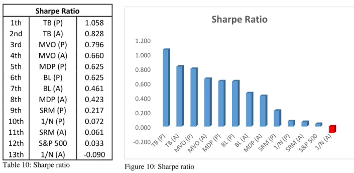
The Treynor-Black model (TB) is an optimization method developed by Jack Treynor and Fischer Black (1973), and was originally published in Journal of Business in 1973. The model is based on a presumption that only securities showcasing abnormal returns are worth adding to an otherwise most efficient portfolio, the market portfolio. If such securities occur and are not yet included in the market portfolio, the market portfolio is no longer efficient. The optimal portfolio suggested by TB is thus a combination of the market portfolio and the active portfolio composed of selected securities with positive abnormal returns. Since the number of securities within the active portfolio is usually limited, the incorporation of the market portfolio also significantly improves the overall diversification. The ability to predict abnormal returns is critical within the TB framework, so to avoid any possible inconsistencies coming from using a variety of different security analyses, the TB assumes the use of the market model characterized by the Equation 3.4. In MM, the abnormal return is represented by non-zero alpha, i.e. 𝛼 ≠ 0. Any rational investor desires and seeks 𝛼 > 0, which delivers superior return to the portfolio. This inequality is important in order to maintain the positive risk-return trade-off as the security always increases the portfolio risk through its own residual variance. The ultimate goal of TB optimization is the maximization of the optimal portfolio’s Sharpe ratio8. The majority of MVO assumptions apply for the TB model as well (Kane et al., 2003).
Let’s assume n+1 assets, where n is the number of securities with abnormal returns forming an active portfolio A and +1 represents the market index as a passive portfolio M, both together forming an optimal portfolio P. The estimates of alpha, beta, and residual variance coefficients on portfolio level are following (Bodie et al., 2018):
𝛼𝑃 = ∑ 𝑤𝑖𝛼𝑖 ; 𝛼𝑀 = 0 𝑛+1 𝑖=1 (4.37) 𝛽𝑃 = ∑ 𝑤𝑖𝛽𝑖 ; 𝛽𝑀 = 1 𝑛+1 𝑖=1 (4.38) 8 𝑆𝑅 =𝐸(𝑟𝑃)−𝑟𝑓 𝜎𝑃
33 𝜎𝜀2𝑃 = ∑ 𝑤𝑖2𝜎𝜀2𝑖 ; 𝜎𝜀2𝑛+1 = 𝜎𝜀2𝑀 = 0
𝑛+1 𝑖=1
(4.39) The formula for optimal weight allocated to the active portfolio A is following:
𝑤𝐴 = 𝐸(𝑟̅ )𝜎𝐴 𝑀 2 − 𝐸(𝑟 𝑀 ̅̅̅)𝜎𝐴𝑀 𝐸(𝑟̅ )𝜎𝐴 𝑀2 + 𝐸(𝑟̅̅̅)𝜎𝑀 𝐴2 − [𝐸(𝑟̅ ) + 𝐸(𝑟𝐴 ̅̅̅)]𝜎𝑀 𝐴𝑀 (4.40) Where 𝑟̅ stands for risk premium. Therefore,
𝐸(𝑟̅ ) = 𝐸(𝑟𝐴 𝐴) − 𝑟𝑓 = 𝛼𝐴 + 𝛽𝐴[𝐸(𝑟𝑀) − 𝑟𝑓] 𝐸(𝑟̅̅̅) = 𝐸(𝑟𝑀 𝑀) − 𝑟𝑓
𝜎𝐴𝑀 = 𝛽𝐴𝜎𝑀2
𝜎𝐴2 = 𝛽𝐴2𝜎𝑀2 + 𝜎𝜀𝐴
2
After plugging all together and proceeding algebraic simplifying manipulations, the allocation to portfolio A gets following:
𝑤𝐴 = 𝑤0 1 + (1 − 𝛽𝐴)𝑤0 ; 𝑤𝑀 = 1 − 𝑤𝐴 (4.41) Where 𝑤0 = 𝛼𝐴/𝜎𝜀𝐴 2 𝐸(𝑟̅̅̅)/𝜎𝑀 𝑀2 (4.42)
is the initial allocation to A if 𝛽𝐴 = 1.
The allocation to n individual securities within the portfolio A is following:
𝑤𝑖 = 𝑤𝐴 ∗ 𝛼𝑖 𝜎𝜀𝑖 2 ∑ 𝛼𝑖 𝜎𝜀2𝑖 𝑛 𝑖=1 (4.43)
As mentioned, the end goal of TB optimization is maximization of the optimal portfolio’s Sharpe ratio (SR). Therefore, as optimal portfolio is a combination of market portfolio and a portfolio of securities with superior expected returns, the overall SR must exceed the one of the market. The exact relationship is following:
34 𝑆𝑅𝑃 = √𝑆𝑅𝑀2 + [𝛼𝐴 𝜎𝜀𝐴] 2 = √𝑆𝑅𝑀2 + ∑ [𝛼𝑖 𝜎𝜀𝑖] 2 𝑛 𝑖=1 (4.44)
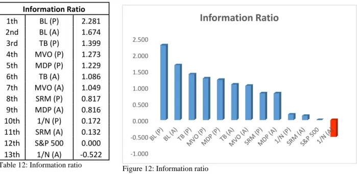
Where the ratio of alpha to its residual SD is called the information ratio. Parameters of optimal portfolio
Risk premium 𝐸(𝑟̅ ) = (𝑤𝑃 𝑀+ 𝑤𝐴𝛽𝐴)𝐸(𝑟̅̅̅) + 𝑤𝑀 𝐴𝛼𝐴 (4.45) Variance 𝜎𝑃2 = (𝑤 𝑀+ 𝑤𝐴𝛽𝐴)2𝜎𝑀2 + (𝑤𝐴𝜎𝜀𝐴) 2 (4.46)
4.3.
Black-Litterman
The Black-Litterman model (BL) is an optimization method developed by Fischer Black and Robert Litterman (1992), and was originally published in Financial Analysts Journal in 1992. Over the time and due to the popularity of BL approach, a number of extensions to BL have been developed. In this thesis, only the original BL model is introduced and used. BL is based on a combination of inverse optimization and Bayesian statistics. It assumes that the optimal portfolio asset weights are known, represented by their weighting in the market index, and then these weights are subjects of adjustments in accord to the investor’s unique views about the future performance of these assets. This is in contrast with MVO, in which the estimates of expected returns are used as a starting point in derivation of optimal weights. Such approach overcomes the major shortcomings of MVO – input sensitivity, high concentration, and estimation error maximization. This brief introduction of BL is based upon the works of Idzorek (2002) and Walters (2014).
The starting point of inverse optimization under BL framework is the derivation of implied equilibrium excess returns, denoted Π, which is a N x 1 column vector resulting from following expression:
35 Where 𝜆 = 𝐸(𝑟𝑀)−𝑟𝑓
𝜎 𝑜𝑓 𝑀 𝑒𝑥𝑐𝑒𝑠𝑠 𝑟𝑒𝑡𝑢𝑟𝑛𝑠2 is the risk-aversion coefficient of market portfolio, Σ is the
covariance matrix of excess returns, and 𝑤𝑚𝑘𝑡 is the market capitalization weight N x 1 column
vector of the assets.
As in MVO, the optimization goal of BL is the maximization of investor’s mean-variance utility
max 𝑈 = 𝑤𝑇𝜇 −1 2𝜆𝑤
𝑇Σ𝑤 (4.48)
⋮
𝑤 = (𝜆Σ)−1𝜇 (4.49)
Where μ is any vector of excess returns. If 𝜇 = Π, then 𝑤 = 𝑤𝑚𝑘𝑡
If an investor possesses no specific views about the future performance of the assets, he should then hold the portfolio with weights derived from the vector of implied equilibrium returns, i.e. 𝑤𝑚𝑘𝑡 , which is the view-neutral starting point of the BL model.
The original BL formula is:
𝐸(𝜇̅) = [(𝜏Σ)−1+ 𝑃𝑇Ω−1𝑃]−1[(𝜏Σ)−1Π + 𝑃𝑇Ω−1𝑄] (4.50)
Where
𝐸(𝜇̅) is the posterior combined return vector (N x 1) 𝜏 is scalar
Σ is covariance matrix of excess returns
P is a (K x N) matrix identifying the assets involved in the views, where K is the number of views and N the number of assets
Ω is a diagonal (K x K) matrix representing the residual variance associated with the expressed views
Q is a (K x 1) column vector of views
Idzorek (2002: 13) describes the BL model as a “complex weighted average of the implied
equilibrium return vector Π and the view vector Q, in which the relative weightings are a function of the scalar τ and the uncertainty of the views Ω.” Although the BL model doesn’t require one to
specify any views, the possible incorporation of investor’s views within the model is perhaps the most attractive feature of the BL model. The views can be expressed either in an absolute or
36 relative form. The absolute view expresses an idea about an absolute return on an asset, e.g. 5%. The relative view expresses an idea about an asset under- or outperforming relatively to some other asset, e.g. asset A outperforms asset B by 25 b.p. The views form Q (K x 1) matrix. The uncertainty about the views is expressed in the error term vector denoted ε, where each error term 𝜀 ~ 𝑁(0, 𝜎2). 𝑄 + 𝜀 = [ 𝑄1 ⋮ 𝑄𝑘 ] + [ 𝜀1 ⋮ 𝜀𝑘] (4.51) The expressed views are linked to the assets in question via the matrix P (K x N)
𝑃 = [
𝑝1,1 ⋯ 𝑝1,𝑛
⋮ ⋱ ⋮
𝑝𝑘,1 ⋯ 𝑝𝑘,𝑛]
(4.52) Where each row is associated with one specific view. If the view is positive, the associated weight has a positive sign, e.g. +1, if negative then -1. The sum of weights in each row must be equal to 0 in case of relative views, and equal to 1 in case of absolute views. The actual weighting used in practice is where multiple versions of the BL model differ. Some weighting schemes use equal weighting, market capitalization weighting, or confidence level based weighting expressed as percentage on an intuitive scale 0-1.
The error terms enter the BL formula in form of its variance, denoted ω, and expressed in the Ω matrix 𝛺 = [ 𝜏𝜔1 0 0 0 ⋱ 0 0 0 𝜏𝜔𝑘 ] (4.53) Where 𝜔𝑘= 𝑃𝑘Σ𝑃𝑘𝑇 (4.54)
The scalar τ should be more or less inversely proportional to the relative weight given to Π. However, its recommended value differs across literature and its variation is one of the ways how to calibrate the model for specific needs. Black and Litterman recommend to use values close to zero, such as often recommended τ=0.0025.
The last step of BL optimization is to obtain the combined return vector 𝐸(𝜇̅), Equation 4.50, and plug it into the Equation 4.49, which returns the optimal portfolio weights.