Calibration and performance of the tile calorimeter of ATLAS with cosmic ray muons

(1)

UNIVERSIDADE DE LISBOA FACULDADE DE CI ˆENCIAS DEPARTAMENTO DE F´ISICA

Calibration and Performance

of the

Tile Calorimeter of ATLAS

with

cosmic ray muons

Jo˜ao Gentil Mendes Saraiva

DOUTORAMENTO EM F´ISICA 2010

(2)

(3)

UNIVERSIDADE DE LISBOA FACULDADE DE CI ˆENCIAS DEPARTAMENTO DE F´ISICA

Calibration and Performance

of the

Tile Calorimeter of ATLAS

with

cosmic ray muons

Dissertac¸˜ao submetida por

Jo˜ao Gentil Mendes Saraiva

com o grau de Mestre em F´ısica

como requesito parcial para a obtenc¸˜ao do grau de Doutor em F´ısica

Dissertac¸˜ao orientada por:

Prof. Doutora Am´elia Arminda Teixeira Maio e

Dr. Jos´e Carvalho Maneira

DOUTORAMENTO EM F´ISICA 2010

(4)

(5)

Agradecimentos

Não posso deixar de agradecer a todos os que ajudaram na execução desta tese. As contribuiç ões para o trabalho e também aquelas que me afastaram dele, sem as quais teria sido muito mais dif´ıcil esta tese ter chegado a bom porto. Os nomes não são segredo nenhum, mas também apenas s ó interessam a mim, por isso curiosos da vida alheia vão ter que ler outra tese.

Agradeço o apoio da Prof. Amélia Maio que embora sempre muito ocupada, não deixa de se preopocupar com todos os seus alunos, e parece por vezes ter mais energia (muito mais do que 14 TeV!) e entusiasmo que todo o grupo de ATLAS junto.

Agradeço ao José Maneira todo o apoio e paciência durante estes anos de tese, e toda a ajuda disponibilizada na realização do trabalho que agora com a escrita desta tese viu o seu fim.

Agradeço ainda ao Nuno Ribeiro, que queria ser te órico quando fosse grande (mas ele já é grande?!) e ao recentemente chegado Mário Sousa, pela grande ajuda que deu o primeiro e tem dado agora o segundo nas análises de dados.

Agradec¸o a todos os que gostaram de fazer um pequeno intervalo no seu dia de trabalho para tomaram caf´e comigo.

Agradeço a todos os meus colegas do grupo de ATLAS no LIP que ajudaram de uma ou outra forma para que esta tese estivesse escrita hoje a um mês do centenário da implantação da republica.

Por fim agradec¸o aos meus pais o apoio que me tem dado ao longo destes intermin´aveis anos de estudante.

(6)

(7)

List of Figures

1.1 The LHC complex where are visible the different stages of preparation of the LHC beam: Linac → Booster → PS → SPS → LHC. The beams are injected in the LHC ring with an energy of 450 GeV. . . 2 1.2 A scheme of the LHC accelerator showing the main characteristics of the two

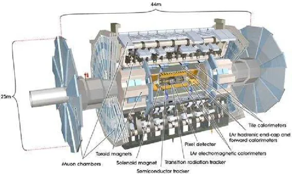
circulating beams: one circulating clockwise and the other anti-clockwise in two separate rings. Close to each of the interaction points there are 140 m long ring segments that are used by both beams. . . 4 1.3 A cut-view scheme of the ATLAS detector showing its main elements and

dimensions. . . 7 1.4 The inner detector of ATLAS: Pixels detector, Semiconductor Tracker and

Transition Radiation Tracker. . . 8 1.5 The ATLAS calorimeters . . . 10 1.6 The accordion geometry of the absorber plates and the honeycomb spacers of

the LAr barrel electromagnetic calorimeter. . . 10 1.7 The muons spectrometer of the ATLAS detector. The different sub-systems are

evidenced the MDT, CSC, RPC and TGC. . . 12 1.8 The Z0boson average mass and width results from LEP-I experiments. . . 18 1.9 The hadronic cross section dependence on the number of light neutrinos

families. The experimental results fit well to the 3ν case which validates that the number of light neutrinos is three. . . 19 1.10 W boson mass and width world average from LEP-II. . . 20

(12)

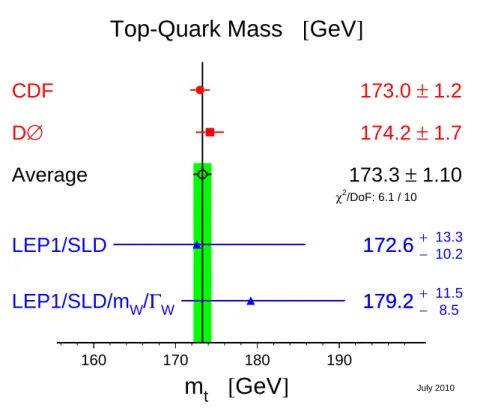
1.11 Top quark mass direct measurement from the Tevatron. Other experiments only have indirect measurement. . . 21 1.12 Higgs boson mass limits. The shaded bands represent exclusion regions for the

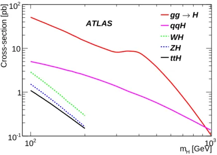
Standard Model Higgs boson mass: MH<114 GeV at LEP experiments [9] and 158 GeV < MH < 175 GeV [7] from TEVATRON at Fermi Lab. . . . 22 1.13 Cross-section for the production of the Higgs boson as function of its mass for

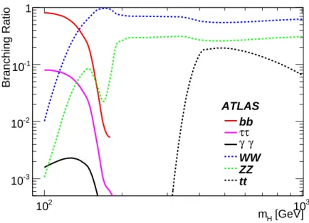
the LHC with √s = 14 TeV. . . . 23 1.14 Branching ratio of the Higgs boson decays as function of its mass for the LHC

with √s = 14 TeV. . . . 24

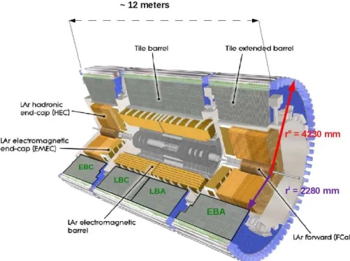
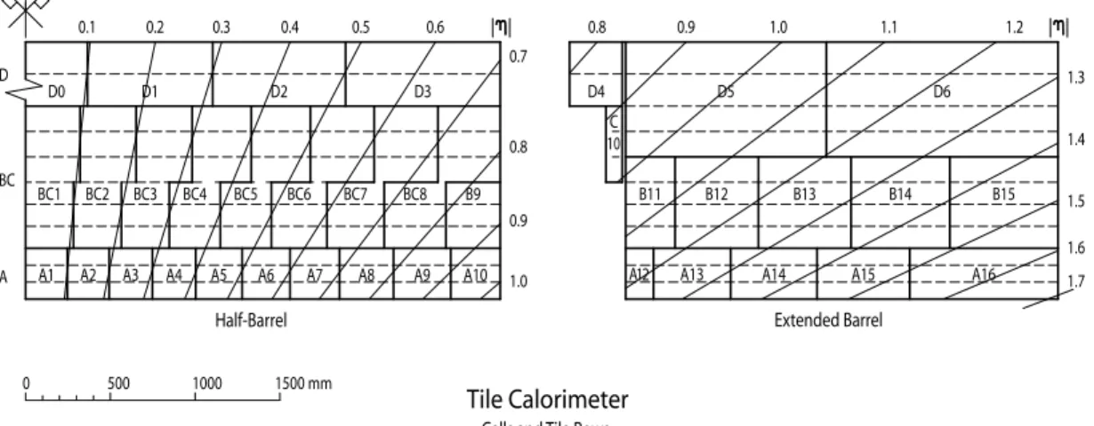
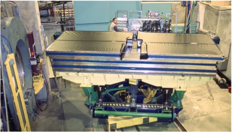
2.1 The Tile Calorimeter partitions: EBA, LBA, LBC and EBC . . . 26 2.2 Tile Calorimeter cells and rows in the RZ plane. . . 27 2.3 Tile Calorimeter module structure: sampling calorimeter with a steel matrix

where scintillating plastic tiles are embedded. The signal produced in each scintillating tile by ionizing particles is double-readout two photomultipliers. The signal is carried to the PMTs by WLS optical fibers. . . 28 2.4 Significance of random triggered events in the tile calorimeter cells. A single

gaussian description of noise ¤ is compared with a double gaussian description △ [18]. . . 32 2.5 The electronic noise in Tile Calorimeter modules measured using the RNDM

stream during a cosmic ray muon on September 2008 [19]. . . 33 2.6 The calibration systems of the tile calorimeter and their interface to the readout

system from scintillating tiles to front-end electronics. . . 34 2.7 Channel-to-channel variation of the high gain (a) and low gain (b) readout

calibration constants C_ADC→pCprior to any correction [18]. . . 36 2.8 Time stability of the average high gain (top) and low gain (bottom) readout

calibration constants from August 2008 to October 2009, for 19,595 ADC channels [18]. . . 37 vi

(13)

List of Figures

2.9 Relative gain variation (to a reference measurement) for the tile calorimeter photomultipliers during a period of 50 days. Each entry in the histogram is a photomultiplier. Shaded areas correspond to relative gains above 1% [18]. . . . 39 2.10 Cesium system working principle. . . 40 2.11 Cesium system measurements in the ATLAS experimental cavern. (a)

The solid lines are the expected decay curves for the cesium sources (one for each cylinder). The experimental points are from Cesium data taken with the magnetic field off and on (with MF close to data points). (b) Normalized response where the up-drift of the Tile Calorimeter absolute value is measured [18]. . . 41 2.12 The Tile Calorimeter up-drift due to the presence of the ATLAS magnetic field.

The ratio between the integrated signal with magnetic field IMand integrated signal without magnetic field I0in η and φ [18]. . . 43

2.13 Integrator response: (a) Gain stability (b) Stability in time during approximately 2 years of monitoring relative to January 2008 (c) Electronic noise. The measurements used 95.3% of the Tile Calorimeter channels [18]. . . 44 2.14 The Tile Calorimeter setup during the 2000 to 2003 standalone testbeam. . . 45 2.15 Electromagnetic energy scale of the Tile Calorimeter for electrons measured

during testbeam. The cell response of electrons entering the calorimeter modules exposed to the beam at incidence angle of 20◦, normalized to beam energy, with one entry for each A-cell measured. The plot contains data at various energies ranging from 20 to 180 GeV [26]. . . 46 2.16 Uniformity in η of 180 GeV muons in MeV/cm. The experimental data are the

filled circles • and Monte-Carlo simulation results are the open squares ¤ [26]. 47 2.17 Separation of signal and electronic noise for 180 GeV muons entering the

(14)

2.18 The Tile Calorimeter standalone energy resolution for pions impinging on the calorimeter at |η| = 0.35 (7.9λ), as a function of the beam energy. MC simulation results (Geant 4.8.3 QGSP+Bertini models) shown with open squares and full circles data [26]. . . 49 2.19 Normalized energy response plotted against the pion energy impinging the

calorimeter for |η| = 0.35. Open squares represent Geant 4.8.3 Monte Carlo simulations, with QGSP and Bertini intranuclear cascade models and full circles data. In the figure on the RIGHT corrections for longitudinal and transverse leakage are introduced [26]. . . 50 2.20 Lateral view of the sub-detectors used in the 2004 combined testbeam. . . 51 2.21 Mean energy (a) and resolution (b) for pions at beam momenta from 2 to 180 GeV

are shown. Data is represented as closed points and Monte Carlo simulations as lines. Only statistical uncertainties are shown. The light band represents the uncertainty due to the cut to remove muons from pion decays. . . 52 3.1 Precision of the online reconstruction with the optimal filter algorithm [18]. . . 57 3.2 Jet time after rejection of fake jets due to noise burst in LAr calorimeter. . . 59 3.3 Difference between the cell time of modules on the top (y > 0) and modules on

the bottom (y < 0) for (a) di-jets MC (b) cosmics MC and (c) cosmics data [31]. . 61 3.4 Velocities (β) for different predicted SMPs in Super-Symmetric models. . . 68 3.5 Timing resolution from testbeam data for cell A-6. . . 69 4.1 The start of the assembly in the ATLAS cavern on March 1st, 2004. The first 8

modules, pre-assembled on the surface, on a cradle. . . 74 4.2 A cosmic ray muon recorded by the ATLAS barrel Tile Calorimeter at 18:30, on

21 June 2005 [36]. . . 76 4.3 The Tile Calorimeter standalone cosmic ray muons trigger setup: coincidence

between top and bottom modules. . . 79 4.4 Expected trigger rates from Monte-Carlo for the Tile Calorimeter standalone

trigger. . . 80 viii

(15)

List of Figures

4.5 ROD and TTC optical fibers attenuation results for two different wavelengths. . 81 4.6 Response from a good optical fiber seen by the OTDR. . . 82 4.7 Typical problems found in optical fibers during the OTDR tests. . . 83 4.8 ROD and TTC optical fibers length results. . . 84 4.9 The distributions of triggers from the trigger board output in early

commis-sioning (2006): 8 modules TOP in the C side and 8 modules BOTTOM in the A side . . . 87 4.10 Tower of maximum energy: TOP and BOTTOM modules. . . 88 4.11 The distribution of the TileCal towers above a 1 GeV tower threshold (300 MeV

cell threshold) probing on all the connected modules during the M4 integration week. . . 89 4.12 The distribution of the TileCal towers above a 1 GeV tower threshold (300 MeV

cell threshold) probing on all the connected modules during the M7 integration week. . . 90 4.13 Charge integrals for the channels of two Tile Calorimeter modules: module 17

and module 15. . . 90 4.14 Digitized signal samples distributions: a symmetric distribution with a peak in

sample 5 for LBC17 and in sample 6 for LBA48 . . . 91 4.15 The technical drawing of the collimator of the LHC accelerator. . . 92 4.16 Details of the collimator’s (a) One of the collimator jaws used in the secondary

collimator that has the same dimensions but it is made of carbon (b) The collimator is opened (c) The collimator is closed. . . 93 4.17 A event display of a splash event in the ATLAS detector. Each splash event

could reach up to a few TeV of deposited energy. . . 93 4.18 Comparing the trajectories of muons in Single Beam data and cosmic ray muons

(16)

5.1 Vertical flux of particles with energy above ¿ 1 GeV in the atmosphere. The lines are estimated values and the points are experimental results from negative

muons with E > 1 GeV [3]. . . . 96

5.2 Distribution of muons at the earth surface [3] (left) and the ATLAS detector in the experimental cavern (right). . . 96

5.3 The ATLAS cavern muon-ray plate. The circular regions with higher statistics represents the ATLAS experimental caver shafts. . . 97

5.4 Typical shape of the muon spectra crossing the Tile Calorimeter detector. The usual quantities used to characterize the muon response are indicated. . . 99

5.5 Energy loss by muons in copper [3]. . . 99

5.6 Tracks detected in a cosmic event. . . 102

5.7 Tracks detected in a single-beam data event. . . 102

5.8 The parameters of the track calculated using the TMF algorithm: a direction given by the angles θ and φ and a point given by the intersection of the track with the plane y = 0. . . 105

5.9 The definition of a track by the tile muon fitter algorithm is based in 2 angles (a) and in the coordinates in the plane XZ for y=0 (b). . . 107

5.10 Angular precision for the zenith angle θ and azimuth angle φ. The histograms entries are per-event differences between the reconstructed and the generated angles. . . 108

5.11 Position precision in the X and Z-coordinate respectively, both at the horizontal plane (Y = 0) crossing. The histograms entries are per-event differences between the reconstructed and the generated angles. . . 109

5.12 Average imbalance < AE > in TileCal modules as a cross-check on energy calibration . . . 111

5.13 Signal and noise separation considering all possible trajectories for the cosmic ray muons. Data and pedestal include exactly the same cells per event. The RNDM stream was used for pedestal and RPC data stream was used for data. . 113 x

(17)

List of Figures

5.14 Energy muon for projective muons selected in 0.3 < η < 0.4. The pedestal distribution uses per event the same selected cells as the ones used for data. The ID-COMM data stream is used for data and RNDM stream used for the pedestal. . . 115 5.15 The effect of sampling fraction with the variation of the θTMF. The data points

on the left for small values of |90 − θTMF| . . . 117 5.16 Cosmic ray muons triggered by the RPCs and momentum measured by the

muon spectrometer. . . 118 5.17 Distribution of energy loss (dE/dx) showing the region eliminated with a 1%

truncation on the high energy tail. . . 119 5.18 Energy loss per radial layer using (a)the TMF for track reconstruction. The

error bars are the systematics errors from Table 5.4 and (b) the IDtrack [18]. . . 121 5.19 Energy loss for the radial layer A using ID-COMM stream data and ratio with

Monte-Carlo simulated data. . . 126 5.20 Uniformity in φ of the energy loss for the three radial layers of LB. The results

combine the two LB partitions LBA and LBC. This option is to compensate for low statistics. The ratio of data points with Monte-Carlo are also given for each radial layer. The Monte-Carlo, as mentioned before, only uses the TRT volume which explains that not all data points have a correspondent data/MC value. . 127 5.21 Weighted average module energy loss for each radial layer of the LB. The results

combine the two LB partitions LBA and LBC. This option is to compensate for low statistics. The results for the two physic stream are presented for comparison.128 5.22 Uniformity in φ of the energy loss for the three radial layers of EB. The results

combine the two EB partitions EBA and EBC. This option is to compensate for low statistics. The ratio of data points with Monte-Carlo are also given for each radial layer. The Monte-Carlo, as mentioned before, only uses the TRT volume which explains that not all data points have a correspondent data/MC value. . 130

(18)

5.23 Weighted average module energy loss for each radial layer of the EB. The results combine the two EB partitions EBA and EBC. This option is to compensate for low statistics. The results for the two physic stream are presented for comparison.131

6.1 Tile Calorimeter cells time measured with single beam 2008 data against the cell coordinate z: (a) Time measured showing slopes that result from the different distances to the collimator (b) Correcting for the time of flight of muons crossing the different calorimeter cells. . . 140 6.2 The cell time against the z coordinate of each cell for different values of vc f. . . 142 6.3 The cell time against the clear fiber length for different values of vc f. . . 143 6.4 A fine scan on vc f: (LEFT) The slope dt/dz vs vc f (RIGHT) the slope dt/dL vs vc f. 144 6.5 The selected < ∆Tα

β >. The individual cells have an energy above 200 MeV

and the time difference between readout channels of a cell is below 6 ns. The cells pairs were required to have more than 5 measurements and a standard deviation lower than 5 ns. . . 152 6.6 Number of measurements per cell (x-axis) and module (y-axis) (a) First radial

layer (A cells) (b) Second radial layer (BC cells) (c) Third radial layer (D cells). . 153 6.7 Number of cells with measured time offsets in function of the set of used cuts. . 157 6.8 Tile Calorimeter towers inter-module synchronization done in the early

commissioning using 2006 data (a) Intra-module synchronized using the laser/led system (b) Inter-module synchronization applied using 2006 cosmic ray muons data. . . 162 6.9 Modules average time from Tile Calorimeter inter-module calibration done in

the early commissioning using 2006 data: • intra-module synchronized using the laser/led system and ⋆ inter-module synchronization applied using 2006 cosmic ray muons data. . . 163 6.10 Tower time offsets for 2008 Cosmic ray muons data: average, standard deviation

and population (number of towers used in obtaining the statistical quantities). 165 xii

(19)

List of Figures

6.11 Tower time offsets for 2008 Cosmic ray muons data: average, standard deviation and population (number of towers used in obtaining the statistical quantities). 167 6.12 Time offsets: average, standard deviation and population (number of cells used

in obtaining the statistical quantities). . . 169 6.13 Time offsets: average, standard deviation and population (number of cells used

in obtaining the statistical quantities). . . 170 6.14 Time offsets measured using cosmic ray muons for each Tile Calorimeter partition.173 6.15 Correlation between the applied faked offsets in the vertical axis and the tnet

shows the independence between the applied fake offset and the retrieved tnet that is used to account for the accuracy and precision of the method. . . 176 6.16 Precision and accuracy for measuring time offsets (tcell_cosmics) using cosmic ray

muons. . . 177 6.17 Long Barrel – Relative accuracy of cosmic ray muons and single beam: module

average and standard deviation. . . 181 6.18 Extended Barrel – Relative accuracy of cosmic ray muons and single beam:

module average and standard deviation. . . 182 6.19 Difference of time offsets seen in the single beam and cosmic ray muons data

for the Tile second and third radial layers for the four Tile Calorimeter partitions.184 6.20 Correlation between the time offsets measured with the 2008 single beam data

and cosmic ray muons data from the same period. . . 187 6.21 Relative accuracy of cosmic ray muons and single beam time offsets

measure-ments. Excluding the first radial layer – A cells – of each Tile Calorimeter partition. . . 189 6.22 Tile Calorimeter cells time measurements from single beam data vs z : (a) single

beam 2009 data (b) single beam 2010 data after using single beam 2009 for cells synchronization. . . 193 6.23 Tile Calorimeter cells time in 2010 after synchronization using single beam data

(20)

(21)

List of Tables

1.1 ATLAS magnetic field main characteristics . . . 8

1.2 Parameters of the muon spectrometer. . . 13

3.1 Selection cuts for the Higgs boson decay to four leptons. The m12 defines a mass window for the first pair of leptons match with the Z boson nominal mass. The m34is the minimum mass required for the second Z boson for Higgs boson masses up to 200 GeV. For higher Higgs boson masses an equivalent mass window for the second lepton pair is applied [10]. . . 64

3.2 Higgs boson to four leptons decay leading order and next to leading order cross sections for different Higgs boson masses (l = e, µ) [10]. . . . 64

3.3 Backgrounds to the Higgs to four leptons decay cross sections. Corrections are introduced as a compensation for diagrams not included in used generators [10]. 65 3.4 Fraction of signal events (%) for each selection cut and for a Higgs mass of 130 GeV [10]. . . 65

3.5 Fraction of events (%) for backgrounds processes for each selection cuts and for a Higgs mass of 130 GeV [10]. . . 66

3.6 Bunch crossing times for some colliders. . . 71

4.1 Milestones of the Tile Calorimeter pre-assembly tests on the surface. . . 74

4.2 Milestones of the Tile Calorimeter assembly in the ATLAS cavern. . . 75

(22)

5.1 The results from a fit with a gauss and landau convoluted function for the module response (A+BC+D) and for each radial layer (RPC data stream). . . . 112 5.2 The signal to noise ratio (S/N) for the average module response and for each

radial layer (RPC data stream). . . 114 5.3 Crossed path length cut values. . . 116 5.4 Systematic error for the energy loss measurement using data from the

ID-COMM physics stream. The total error is the quadratic sum of the different contributions. The Global EM scale factor is the one included in the Tile Calorimeter readiness paper for collisions [18] . . . 122 5.5 Systematic error for the energy loss measurement using data from the RPC data

stream. The total error is the quadratic sum of the different contributions. The Global EM scale factor is the one included in the Tile Calorimeter readiness paper for collisions [18] . . . 123 5.6 Energy loss 1% truncated mean [MeV/mm] for ID-COMM. The errors are

systematic uncertainties from Table 5.4. Results from 2000-2003 testbeam for 11-20 GeV/c muon spectra. The double ratio divided Data/MC from cosmics with Data/MC from testbeam (Eq. 5.2). . . 123 5.7 Truncated mean and the systematic uncertainties [MeV/mm] for RPC data stream.125 5.8 Long barrel uniformity results for the RPC data stream and the ID-COMM stream.126 5.9 Extended barrel uniformity results for the RPC data stream and the ID-COMM

stream. . . 129

6.1 Clear fiber lengths for each photomultipliers of the Tile Calorimeter long barrel and corresponding relative time corrections. . . 138 6.2 Clear fiber lengths for each photomultipliers of the Tile Calorimeter extended

barrel and corresponding relative time corrections. . . 139 6.3 Speed of light in clear fibers in the four Tile Calorimeter partitions. . . 144 6.4 Speed of light in clear fibers in the four Tile Calorimeter partitions. . . 146 xvi

(23)

List of Tables

6.5 Number of quantities needed to identify an instrumental unit (IU) in Tile Calorimeter. Depending on the IU choice α and β must take in account these set of parameters to identify unambiguously the IU. . . 148 6.6 Use of + or − signal in Equation 6.6 depending on the chosen reference position

and the φ coordinate. . . 149 6.7 Instrumental units selection cuts. . . 151 6.8 Maximum number of rows – equations – and maximum number of columns –

unknowns. The number of rows corresponds to the number of possible pairs of cells. The number of columns to the number of cells. In this account the scintillators readout by the Tile Calorimeter FEE are not included. . . 156 6.9 Comparison of lists of solutions with combined results (left) and reference

results (right) for GEOM lists selection. . . 159 6.10 Comparison of lists of solutions with combined results (left) and reference

results (right) for CPID lists selection. . . 159 6.11 Comparison of lists of solutions with combined results (left) and reference

results (right) for COUN lists selection. . . 160 6.12 Agreement of the combined list with reference list. . . 160 6.13 Tower time offsets measured with cosmic ray muons 2006 data. Each column

represents the time offset for a tower in a module. The index 1 refers to tower η = 0.05 and so forth. . . 163 6.14 Tower time offsets measured with cosmic ray muons 2006 data after correcting

the time constants using the results from Table 6.13. Each column represents the time offset for a tower in a module. The index 1 refers to tower η = 0.05 and so forth. . . 164 6.15 Average and RMS for tower time offsets using 2008 cosmic ray muons data in

the Tile Calorimeter partitions. The 16 most vertical module span from module 9 to 24 on the top (y > 0) and from module 41 to 56 on the bottom (y < 0). Results are also shown selecting the 12 most vertical modules. . . 166

(24)

6.16 Time offsets difference between 2008 Single beam data and 2008 Cosmic ray muons data. The results are summarized per partition using only the most vertical modules as: mean (RMS). . . 168 6.17 Number of cells per partition and cell type for which time offsets were

calculated. The total number of cells existing in the Tile Calorimeter are 1920 for layer A, 1920 for layer B/C and 832 for layer D. The scintillators are not included in these numbers. (∗)For the D cells of LBA are also included the 59 D0 cells measured. . . 171 6.18 Average time offsets detailed per radial layer. . . 172 6.19 Time offsets measured using cosmic ray muons data for each Tile Calorimeter

partition. . . 173 6.20 Sensitivity on the measurement of a time offset for a BC cell. . . 175 6.21 Accuracy and precision of the tcell

cosmics measurement using cosmic ray muons data per partition. . . 178 6.22 Accuracy and precision of the tcell

cosmicsmeasurement detailed per Tile Calorimeter radial layer and partition. . . 178 6.23 Population and precision per partition for an accuracy between [-0.5,0.5] ns. . 179 6.24 Population and precision per partition and radial layer for an accuracy between

[-0.5,0.5] ns. . . 180 6.25 Number of cells per layer with a time calibration offset measurement. The CMD

data are given for two sets of cuts (1) Number of measurements of ∆Tβ_α≥ 5 and (2) Number of measurements of ∆Tαβ≥ 7. For both the standard deviation was

required to be below 5 ns. The SBD was filtered using a 3 × σ cut. . . 183 6.26 Relative accuracy of cosmic ray muons and single beam time offsets

measure-ments. . . 185 6.27 Relative accuracy and precision of cosmic ray muons and single beam time

offsets measurements detailed per radial layer. . . 186 xviii

(25)

List of Tables

6.28 Relative accuracy of cosmic ray muons and single beam time offsets measure-ments. Excluding the first radial layer – A cells – of each Tile Calorimeter partition. . . 188 6.29 Results from a gaussian fit between [-5,5] ns for the relative accuracy of cosmic

ray muons and single beam time offsets measurements. Excluding the first radial layer – A cells – of each Tile Calorimeter partition. . . 190 6.30 time offsets measured using cosmic ray muons data for each Tile Calorimeter

partition from cells of the second (BC cells) and third (D cells) radial layers. . . 191 6.31 Summary of time offsets measurements from single beam [30] and cosmic

ray muons. For cosmics the time offsets are given for ALL radial layers and excluding the first radial layer (A cells). . . 192

(26)

(27)

Sum ´ario

A instalação do detector ATLAS na caverna experimental, decorreu entre 2005 e 2009. Durante este per´ıodo, técnicos, engenheiros e f´ısicos trabalharam arduamente na preparação do detector para o seu principal objectivo: estudar a f´ısica de altas energias nas novas fronteiras definidas pela mais elevada energia de centro de massa (14 TeV) e alta luminosidade (1034_cm−2_s−1 _{nominal) em experiências de colisionadores. Esta tese inscreve-se no contexto}

deste ambiente intenso e motivador que envolveu todos os membros de ATLAS na preparação do detector para colis ões protão-protão i.e. durante o periodo de certificação com mu ões de radiação c ósmica e os sistemas de calibração e monitorização do detector. Em 2008 durante o per´ıodo conhecido como singlebeam mu ões resultantes da colisão de um feixe prot ões contra colimadores do LHC, foram utilizados para avaliar o desempenho do detector. Este trabalho foi fundamental para preparar o detector para as primeiras colis ões no LHC que começaram em Novembro de 2009.

Antes das colis ões começarem, as únicas part´ıculas de altas energias dispon´ıveis para estudar o desempenho dos detectores do LHC eram os mu ões produzidos na interacção das part´ıculas c ósmicas com os mais altos estratos da atmosfera. Estes mu ões c ósmicos são as únicas part´ıculas que é poss´ıvel detectar e que chegam à superf´ıcie terrestre em n úmero suficiente para poderem ser utlizadas em estudos de desempenho dos diferentes sub-sistemas do detector ATLAS. O trabalho desenvolvido por mim durante o meu doutoramento e que será detalhadamente neste documento foca a calibração em energia e sincronização do calor´ımetro hadr ónico de telhas cintilantes de ATLAS (TileCal) utilizando os mu ões c ósmicos. Estes dois t ópicos de estudo são agora apresentados sumáriamente:

(28)

A escala de energia electromagnetica foi determinada durante os testes com feixes de part´ıculas utilizando apenas 12% do n úmero total de m ódulos. De forma a medir com um método independente a escala de energia electromagética e avaliar a resposta do detector em função de η e φ, aplicado agora a todos os m ódulos do calor´ımetro TileCal, são utilizados mu ões c ósmicos. A minha contribuição consistiu em validar a escala de energia global e a uniformidade da resposta em energia em φ utilizando o algoritmo TileMuonFitter. O método descrito neste documento permitiu validar a escala de energia, inter-calibrada com o sistema de calibração com césio, com uma precisão melhor que 5% e medir uma uniformidade também melhor que 5%. Uma diferença de 3% entre a camada radial A e a camada radial D foi medida, indicando a necessidade de prosseguir os estudos da escala de energia utilizando agora mu ões isolados. Estes resultados obtidos com um método independente estão consistentes com uma análise anterior, descrita no artigo de readiness para colis ões do calor´ımetro TileCal [18]. Embora os calor´ımetros não sejam desenhados e constru´ıdos para detectarem mu ões, estas part´ıculas elementares são de uma grande importância não s ó para a certifica¸cão dos detectores do LHC mas também no programa de f´ısica do LHC. Antes de chegarem às camâras do espectr ómetro de mu ões, os mu ões produzidos como resultado das colis ões protão-protão (p-p) do LHC vão perder energia nos calor´ımetros, sendo necessário introduzir correcç ões nos algoritmos de reconstrução. Estas correcç ões são aplicadas a todos os mu ões que atravessam o calor´ımetro e em particular em processos fundamentais para a calibração de alto n´ıvel do detector que inclui a reconstrução de objectos complexos como o bosão Z no seu decaimento para dois mu ões. Técnicas de isolamento são utilizadas no designado canal-de-ouro para a descoberta do bosão de Higgs, em que o bosão de Higgs decai para quatro lept ões H → ZZ → 4l e onde o isolamento de mu ões utilizando os calor´ımetros desempenha um papel importante na eliminação do fundo de QCD. A resposta do TileCal a mu ões poderá ter um impacto relevante na descoberta de nova f´ısica para além do modelo padrão, como a de modelos Super-Simétricos, e em particular nos testes de modelos onde se inclui a procura de part´ıculas estáveis e de massa elevada, sendo que é esperado que algumas destas part´ıculas massivas, xxii

(29)

devido à sua elevada massa, tenham um desempenho semelhante ao dos mu ões. O trabalho desenvolvido com mu ões c ósmicos não s ó é importante para a certificação do detector como pode ainda ser relevante para a f´ısica do LHC no detector ATLAS. Compreeder a resposta dos mu ões no calor´ımetro TileCal assim como ter sob controlo a escala de energia electromagnetica são pontos fundamentais para se obter o melhor desempenho do detector ATLAS.

Sincronizac¸ ˜ao do calor´ımetro TileCal

A sincronização do calor´ımetro TileCal foi efectuada durante 2008 combinando mediç ões do sistema de calibração com laser e com part´ıculas de alta energia: mu ões c ósmicos e mu ões de colis ões do feixe com colimadores do LHC single beam. No meu trabalho de tese realizei estudos com os mu ões provenientes destas tuas fontes mas com diferentes objectivos. Utilizando dados do single beam mediram-se correcç ões à velocidade de propagação da luz nas fibras ópticas, um dos parâmetros utilizados na sincronização com laser. O valor medido de 18.5 cm/ns levou a uma actualização deste parâmetro do sistema de calibração com laser. O trabalho realizado com mu ões c ósmicos consistiu na determinação das correcç ões de tempo quer para torres (agrupamento de células) quer para células individuais. Estas correcç ões não são mais do que os desvios de tempo que ainda existem mesmo ap ós a a sincronização com o sistema de laser. Os resultados finais mostraram que as mediç ões com os mu ões c ósmicos e com o single beam têm um acordo melhor do que 2 ns. A medição do tempo de um evento é fundamental para o funcionamento do detector e todos os sistemas tem que estar internamente sincronizados e sincronizados externamente com o rel ógio do LHC ( f = _{25 ns}1 dado pelo cruzamento de pacotes do feixe p-p). No calor´ımetro TileCal o tempo tem um papel importante na reconstrução em energia devido aos constrangimentos severos de operação do LHC que apenas permitem uma iteração na reconstrução do sinal. O tempo de cada um dos 10000 canais do TileCal tem de ser conhecido com a precisão de alguns nanosegundos de forma que os coeficientes correctos sejam utilizados pelo algoritmo de Optimal filter na única iteração dispon´ıvel. A medição do tempo é tambem importante para: seleccionar part´ıculas que vêm de colis ões p-p, definir a qualidade de um evento e é ainda a quantidade mais sens´ıvel para a descoberta de part´ıculas lentas e de massa muito elevada que são previstas

(30)

Esta tese divide-se em 7 cap´ıtulos. O primeiro é introdut ório e apresenta o acelerador Large Hadron Collider, o detector ATLAS e os objectivos globais de f´ısica. No segundo cap´ıtulo o calor´ımetro TileCal é descrito com algum promenor apresentado a geometria, os sistemas de calibração e os resultados de desempenho em testes com feixes de part´ıculas. O terceiro cap´ıtulo apresenta as motivaç ões para a análise desenvolvida centrando a discussão na escala de energia e sincronização em tempo do calor´ımetro TileCal. Para além do interesse intr´ınseco para o pr óprio calor´ımetro TileCal, também é discutido o papel que estas quantidades têm no funcionamento de todo o detector, assim como em alguns canais de f´ısica particulares. No Cap´ıtulo 4 a fase de certificação do detector é apresentada, focando algumas das actividades desenvolvidas neste per´ıodo, com destaque naquelas em que dei a minha contribuição durante o desenvolvimento do meu trabalho de tese. A parte central do trabalho de tese encontra-se nos dois cap´ıtulos seguintes. No Cap´ıtulo 5 são apresentados os resultados sobre a escala de energia electromagnética e uniformidade em φ utilizando o algoritmo TileMuonFitter. O Cap´ıtulo 6 é dedicado aos metodos utilizados na sincronização do detector com dados de mu ões c ósmicos e respectivos resultados. Por fim no Cap´ıtulo 7 são apresentadas as conclus ões do trabalho desenvolvido.

Palavras chave:calorimetria, commissioning, mu ões, uniformidade, sincronização

(31)

Summary

The installation of the ATLAS detector in the experimental cavern, took place from 2005 until 2009. During this period, technicians, engineers and physicists have been intensively working on the preparation of the detector for its main objective: probing the new frontiers of high energy physics with the LHC, the particle collider with the largest center of mass energy (14 TeV nominal) and very high luminosities(1034cm−2s−1nominal). The context of this thesis was this challenging environment that involved all ATLAS members in the preparation of the detector for collisions during the period of the detector commissioning with cosmic ray muons and with calibration and monitoring systems. In 2008 during a short period of time single beam data was available and was used to study the detector response. This large effort was fundamental to prepare the detector for the first collisions at the LHC that started in November 2009.

Before collisions started, the only high energy particles available for studies with the LHC detectors were the muons produced by the interaction of cosmic particles in the atmosphere. These cosmic ray muons are the only detectable particles reaching the earth surface in quantities large enough to study the performance of the different sub-systems of the ATLAS detector. The work I have developed during my PhD and that will be detailed in this document is centered on the energy calibration and synchronization of the Tile Calorimeter, the barrel hadronic calorimeter of ATLAS, using cosmic ray muons. The two main topics of study are now summarized:

(32)

A electromagnetic energy scale was set in testbeam using high energy particles for 12% of the Tile Calorimeter modules. My contribution was centered in the validation of the global energy scale algorithm and the detector’s energy response uniformity in φ using the TileMuonFitter. The results presented in this document have shown that both the energy scale application, from testbeam to all modules in the experimental cavern, and the energy uniformity in φ are better than 5%. A difference between radial layers A and D of 3% is measured and it is something not completely understood and must be studied later using e.g. isolated muons from collisions. The used data stream and method, still have shown that a full coverage in φ can be achieved for these measurements. These results obtained with an independent method are consistent with an earlier analysis, reported in the readiness paper of the Tile Calorimeter [18]. Calorimeters are not designed and developed for the detection of muons however they play an important role on the commissioning of the LHC detectors and physics program. Before reaching the muon chambers the muons produced in collisions will lose energy in the calorimeter volume. Corrections on the energy loss in the calorimeters are necessary to improve the precision of the muon momentum measurement. This correction mus be applied to any muons crossing the calorimeter volume and in particular in fundamental processes used on the final calibration of the detector which includes complex objects as the Z boson decaying to two muons. Lepton isolation techniques are used in the so called golden-channel for the Higgs boson discovery, the decay to four leptons H → ZZ → 4l, for the rejection of QCD background. The Tile Calorimeter performance with muons can have an important impact in physics beyond the standard model, such as Super-Symmetry, for instance on the search for stable massive particles, since some of these massive particles are characterized by having an energy loss in the calorimeter similar to muons. The work developed with cosmic muons can also be applied later using muons produced in collisions to monitor the EM scale during the LHC operation. So the work developed with cosmic ray muons is not only important for the commissioning of the detector but can also be relevant for the physics of the LHC to be done with the ATLAS detector. Understanding the response xxvi

(33)

of the Tile Calorimeter to muons as well as to have under control the EM energy scale are fundamental to achieve the best performance of the ATLAS detector.

Synchronization of the Tile Calorimeter

The Tile Calorimeter synchronization was established during 2008 combining measurements with the laser system and high energy particles: cosmic ray muons and muons from single beam. The work presented in this thesis uses both types of muons, but with different objectives in mind. Using the single beam data were measured corrections to the velocity of propagation of light in the clear fibers, a parameter used in the laser synchronization. The measured value of 18.5 cm/ns resulted in the update of this parameter in the laser calibration system. The work done with cosmic muons consisted in the determination of the time offsets of the Tile Calorimeter measured both for towers and individual cells. The time offsets were calculated as the residuals after the synchronization made with the laser system. The final results have shown that the cosmic ray muons and single beam data agree within less than 2 ns. The timing is fundamental for the operation of the detector and all systems must be internally synchronized and externally synchronized with the LHC clock ( f = _{25 ns}1 given by the bunch crossing). The timing plays an important role in the energy measurement due to the stringent operation conditions of the LHC that require the online signal reconstruction for the Tile Calorimeter channels to be done without iterations. The time of each channel must be known with a precision of the order of a few nanoseconds so that the correct parameters are chosen for the online reconstruction method. Time is also used to select particles that come from p-p collisions, to provide quality factors on the selection of events, and it is the most sensitive quantity for the discovery of slow long lived particles, also called stable massive particles, that are predicted in models beyond the Standard Model.

This thesis is divided in 7 chapters. The first is introductory and presents the Large Hadron Collider, the ATLAS detector and its physics goals. In Chapter 2 the Tile Calorimeter is described in some detail presenting the geometry, calibration systems and performance

(34)

the motivations for the work developed, focusing on the energy scale and synchronization of the Tile Calorimeter. These quantities are of course important in the overall detector performance and have also a larger importance in specific physics channels. Chapter 4 introduces the commissioning and gives a brief overview of the activities during this stage, it is mostly descriptive but also reporting with some detail the activities in which I contributed during the development of my thesis work. The main contributions to the Tile Calorimeter commissioning is included in the next two chapters. Chapter 5 presents the results on the energy scale and uniformity in φ using the TileMuonFitter. Chapter 6 is dedicated to the methods and results for synchronization with cosmic ray muons data. Finally in Chapter 7 conclusions are given.

Keywords: calorimetry, commissioning, muons, uniformity, synchronization

(35)

1 Introduction

This thesis is focused on studies with cosmic ray muons of the performance of the hadronic barrel calorimeter of the ATLAS experiment [1], built to detect high energy events at the Large Hadron Collider [2] at CERN. This chapter presents the main elements that build up the background in which my work fits in and the global motivations for the development and construction of this collider and these experiments. Later and in a dedicated chapter (Chapter 3) the direct motivations of my work for the ATLAS experiment are discussed.

1.1 The Large Hadron Collider at CERN

The LHC collider and detectors are the largest and most complex scientific experiment, that was ever built by mankind. The number of people involved, hardware parameters, and goals are well above those of any others experiments that built until now. All this to explore the structure of matter and explain the interactions of the elementary particles by colliding bunches of protons from where physicists may reach for an answer to the still open questions in the field of particle physics.

1.1.1 The accelerator

The accelerators complex that produces the 450 GeV beam injected in the Large Hadron Collider (LHC) is shown in Figure 1.1. The LHC is a two-ring-superconducting-hadron accelerator and collider installed in the ∼ 27 km tunnel that, between 1989 and 2000, hosted the LEP e+e−accelerator. This is a particle-particle collider and two rings with counter-rotating beams are required unlike particle-antiparticle colliders that need only one ring. Figure 1.2

(36)

Figure 1.1: The LHC complex where are visible the different stages of preparation of the LHC beam: Linac → Booster → PS → SPS → LHC. The beams are injected in the LHC ring with an energy of 450 GeV.

(37)

1.1 The Large Hadron Collider at CERN

illustrates this feature by showing the clockwise beam in red and the anti-clockwise beam in blue. Other technical aspects are also indicated such as the injections points where the 450 GeV beam is introduced in the LHC rings, cleaning regions and dumping exits.

The LHC was designed to operate in proton-proton collisions with center of mass energies of up to 14 TeV and luminosities up to L = 1034_cm−2_s−1_{. Each beam can have up}

to 2808 bunches (+ 756 empty bunches), each bunch has 1.15 × 1011_{protons and a length of}

7.55 cm. The crossing angle between beams is 285 µrad. For a fill with the nominal design parameters, the beam bunches collide every 25 ns and give rise to an average of 23 inelastic collisions per bunch.

The rate of events produced in a collision can be calculated as:

Nevent=Lσevent

where σeventis the cross section of the relevant physics process and L is the machine luminosity. The luminosity can be calculated from machine parameters as:

L = N

2

bnb frevγr 4 π ǫnβ_∗ · F

where Nb is the number of particles per bunch, nb the number of bunches per beam, frev the revolution frequency, γrthe relativistic gamma factor, ǫnthe normalized transverse beam emittance, β∗the beta function at the collision point, and F the geometric luminosity reduction

factor due to the crossing angle at the interaction point (IP). This last factor is

F = Ã 1 + µ_θc_σz 2 σ∗ ¶2!−1/2

where θcis the full crossing angle at the IP, σzthe RMS bunch length, and σ∗the transverse

RMS beam size at the IP.

Protons are not elementary particles so in the inelastic collisions the particles the interacting will be its constituents the partons (quarks, gluons). An effective center of mass

(38)

Figure 1.2: A scheme of the LHC accelerator showing the main characteristics of the two circulating beams: one circulating clockwise and the other anti-clockwise in two separate rings. Close to each of the interaction points there are 140 m long ring segments that are used by both beams.

(39)

1.1 The Large Hadron Collider at CERN

energy must be defined:

√

se f f = 2 x1x2

√ s where xi the fraction of momentum carried by each parton.

1.1.2 The detectors

The LHC has two general-purpose and high luminosity experiments ATLAS and CMS having a peak luminosity of L = 1034cm−2s−1 and three low luminosity experiments LHCb with L = 2 × 1032cm−2s−1, TOTEM with L = 2 × 1029cm−2s−1 and LHCf optimized for operation below L < 1030cm−2s−1for p-p collisions at √s = 14 TeV. It has still one experiment dedicated to ion collisions that aims at L = 1027cm−2s−1 for nominal lead-lead ion operation. For the ion-ion collisions the center of mass energy is of √s = 5.5 TeV per nucleon

ATLAS and CMS are competing experiments, since their global objectives are the same. Although competitive, both experiments require that when a measurement is observed in one of them, a confirmation is required from the other. So both must be complementary in order and specially to evaluate any discovery. It is common to refer them as experiments with a general purpose and their physics goals are presented later in this chapter. This designation is attributed in opposition to the other LHC experiments:

• LHCb that is dedicated to the precise measurement of CP-violation in the B-meson system.

• TOTEM that is dedicated to the measurement of the total cross section of elastic proton scattering, with an absolute error of 1 mb, and diffractive dissociation over a wide range of momentum transfer.

• LHCf that is dedicated to the measurement of neutral particles emitted in the very forward region of |η| > 8.4 with the goal of providing data for calibrating the hadron interaction models that are used in the study of Extremely High-Energy Cosmic-Rays. • ALICE was designed for ion-ion collision and will have as main focus the study of the

(40)

and provide a deeper understanding of quantum chromodynamics. However, ALICE also proposes to use proton-proton collisions, both to compare with the ion collisions as well as in physics areas where it can be competitive with the other LHC experiments.

1.1.3 Present status

The operating conditions for the present year (2010) and until the end of 2011 are a center of mass energy of ∼ 7 TeV and a luminosity of the order of 1031 _cm−2 _s−1_{. At the time of}

writing 162 × 109collisions have occurred and a integrated luminosity of ∼ 2.3 pb−1have been accumulated.

1.2 The ATLAS detector

ATLAS is one of the general purpose detectors built for the LHC experiment. The detector is divided in four main units as is characteristic of most high energy particle detectors: a magnetic field, an inner tracker, a calorimeter and a outer tracker. Each one of these units has a set of sub-systems that are responsible for a specific task. Figure 1.3 shows a cut-view of the full detector, from where the different elements mentioned can be depicted. ATLAS measures 44 m in length and 25 m in height and weighs about 7000 tonnes.

1.2.1 Magnetic field systems

The magnetic field in ATLAS is produced by the composition of three systems: the solenoid, the barrel toroid and the end-cap toroid. Their main characteristics are summarized in Table 1.1. The magnetic field will deflect particle’s trajectories according to their mass and charge, this is fundamental for an unambiguous determination of the particle’s type and charge. The solenoid encloses the ATLAS inner trackers and has a magnetic field peak strength of about 2 Tesla.

The two toroids systems are located outside the calorimeters and between the muon chambers that are the sensitive parts of the outer tracker. The combination of these two systems builds up what is called the muon spectrometer and is mainly used for the reconstruction of 6

(41)

1.2 The ATLAS detector

Figure 1.3: A cut-view scheme of the ATLAS detector showing its main elements and dimensions.

muons and their characterization. However, some models beyond the standard model predict the existence of exotic particles of either electromagnetic or hadronic nature, that may reach the outer parts of the ATLAS detector and leave hits in the muon chambers.

1.2.2 Inner tracker

The ATLAS inner tracker is composed of three different detectors: the silicon pixel tracker (Pixels), the transition radiation tracker (TRT) and the semiconductor tracker (SCT), shown in Figure 1.4. The three systems combined cover a region of |η| < 2.5 and have a target resolution for the momentum of

σ(pT)

pT = 0.05% pT ⊕ 1%

To identify tracks and measure their momentum, are challenging tasks under the high multiplicity environment of p-p collisions at nominal LHC luminosity. With an average of 23 collisions more than 1000 particles are produced each bunch-crossing (every 25 ns),

(42)

Solenoid Barrel Toroid End-cap Toroid

Length 5.3 m 25.3 m 5 m

Outer Diameter 2.63 m 20.1 m 10.7 m

Coils

1 coil 8 coils with individual cryostat

2×8 coils with common cryostat

Nominal current 7.73 kA 20.5 kA 20.5 kA

Peak filed strength 2 T 3.9 T 4.1 T

Stored energy 39 MJ 1100 MJ 2×250 MJ

Thickness 0.66 X0 — —

Table 1.1:ATLAS magnetic field main characteristics

Figure 1.4: The inner detector of ATLAS: Pixels detector, Semiconductor Tracker and Transition Radiation Tracker.

(43)

producing a high track density that must be scrutinized to identify the tracks belonging to the interesting event. In addition, the inner detector has the task of measuring the position of event vertex and contribute to the electron identification.

The precision tracking detectors, the SCT (6.3 million channels) and Pixels (80.4 million channels), cover the region of |η| < 2.5. Their arrangement varies depending on the position in η and they are segmented in R − φ and z. Closer to the interaction point they are arrange in concentric cylinders around the beam axis while in the end-cap regions they are located on disks perpendicular to the beam axis. The intrinsic accuracies for the Pixels are: in the barrel 10 µm in R − φ and 115 µm in z and in the end-cap 10 µm in R − φ and 115 µm in R. For the SCT the intrinsic accuracies are: in the barrel 17 µm in R − φ and 580 µm in z and in the end-cap 17 µm in R − φ and 580 µm in R. Typically the Pixels have three space points per track and the SCT 4 space points.

In the TRT (315000 channels) typically 36 hits per track are produced that enables track reconstruction up to η < 2.0. These are 4 mm straw tubes: 144 cm long positioned parallel to the beam axis in the barrel region and 37 cm arranged radially in wheels perpendicular to the beam axis. The intrinsic accuracy is of 130 µm per straw.

1.2.3 Calorimeters

The electromagnetic calorimeter is used to stop and detect the electromagnetic components of the particle’s decays and measure showers produced electrons and photons. This is crucial for the separation of particles that produce electromagnetic showers from the ones producing hadronic jets. The latter are stopped and their properties measured using the hadronic calorimeters. In most cases the deposited energy by hadrons is divided between the two calorimeter systems and a combined reconstruction is necessary.

The electromagnetic calorimeter is a sampling calorimeter using Liquid Argon (LAr) as the sensitive material and lead as the absorber. It has an accordion (Figure 1.6) geometry motivated by the desire to eliminate projective azimuthal cracks that contribute to the constant term of the electromagnetic energy resolution. An early design requisite was a constant term

(44)

Figure 1.5: The ATLAS calorimeters

Figure 1.6: The accordion geometry of the absorber plates and the honeycomb spacers of the LAr barrel electromagnetic calorimeter.

(45)

of 0.7% or less to provide the best possible energy resolution for high-energy electromagnetic objects, as was the case for the H0→ γγ channel. Currently in the Higgs boson mass searches this is not the most sensitive discovery channel due to the limits set to the Higgs boson searches at LEP. The design resolution is

σ(E) E =

10% √

E + 0.7%

It has 3 longitudinal samples covering a region of |η| < 2.5 and a preshower detector covering a region of |η| < 1.8. It has 173 000 channels in the readout.

The hadronic calorimeter uses two different technologies to sample the signal from hadronic jets. In the barrel, covering a region of |η < 1.7|, is the scintillator tile calorimeter (Tile Calorimeter) that has 3 mm scintillating tiles as the sensitive medium and steel as the absorber, using approximately 10 000 channels in the readout (more details are given on the Tile Calorimeter in the dedicated Chapter 2). The end-cap and forward hadronic calorimeters that cover the region of |η| > 1.7 use the same technologies as the electromagnetic calorimeter but with copper (Cu) as the absorber, in the end-cap region and tungsten (W) as the absorber in the forward region. The end-cap has 4 longitudinal samples and the forward 3 longitudinal samples and they have approximately 10 000 channels in the readout. The design resolution for the hadronic calorimetry depends on the |η| region and are defined based on performance requirements for the ATLAS physics goals on the reconstruction of jets:

σ(E) E = 50% √ E + 3% η < 3 and σ(E) E = 100% √ E + 10% η > 3

The calorimeters are readout by the Level 1 trigger to define regions-of-interest that are later communicated to the Level 2 trigger.

(46)

Figure 1.7: The muons spectrometer of the ATLAS detector. The different sub-systems are evidenced the MDT, CSC, RPC and TGC.

1.2.4 Muon Spectrometer

The outermost detector is used for the collection of the charged particles that escape the calorimeter volume. Within the present knowledge of particle physics the only particles reaching these chambers produced in proton-proton collisions are the muons from decays of the collisions products. The measurement and identification is made combining the muon chambers with the barrel toroid magnetic field in |η| < 1.4 and the end-cap toroid in |η| > 1.6. The intermediate region uses the combination of the two magnetic fields to bend the particles. The design momentum resolution requirement for muons is

σpT

pT = 10% at pT = 1TeV

The muon spectrometer is divided in two main parts: the high precision tracker systems and the triggering systems. The characteristic parameters of these systems are listed in Table 1.2 The precision trackers include the Monitored drift tubes (MDT) for most of the η 12

(47)

MDT

Coverage η < 2.7 (innermost layer: η < 2.0)

Number of chambers 1150

Number of channels 354 000

Function Precision tracking

CSC

Coverage 2.0 < η < 2.7

Function Precision tracking

RPC

Coverage η < 1.05

Function Triggering, second coordinate

TGC

Coverage 1.05 < η < 2.7 (2.4 for triggering)

Function Triggering, second coordinate Table 1.2:Parameters of the muon spectrometer.

range and Cathode strip chambers (CSC) for 2 < |η| < 2.7. The latter have a larger granularity, necessary to handle the larger rate of particles in the forward region. In the triggering systems, providing bunch crossing identification and well defined pTthresholds, are the Resistive plate chambers (RPC) in the barrel region and the Thin gap chambers (TGC) in the end-cap region covering the region of |η| < 2.4. These chambers still contribute to the track reconstruction and momentum measurement by measuring the muon coordinate in the direction orthogonal to the one determined by the precision tracking chambers.

1.2.5 Trigger and DAQ system

The trigger system is divided in three levels: L1, L2 and event filter. The L1 selection is hardware based but the other two are already software based.

The collisions occur every 25 ns which means that the L1 trigger will receive data at a rate of 40 MHz. The L1 trigger combines the information from calorimeters (L1-Calo) and

(48)

the muon spectrometer (L1-Muon). It will search for high transverse momentum muons, electrons, photons, jets, and τ-leptons as well as a large missing and total transverse energy. The L1 defines one or more regions of interest in (η, φ) that later are passed to the next trigger levels. It is required that the L1 trigger takes a decision in 2.5 µs reducing the rate to 75 kHz. The L2 trigger uses the ROIs defined by the L1 trigger, runs its algorithms and with its event selection, should reduce the trigger rate to approximately 3.5 kHz, with an average event processing time of 40 ms. The event filter will make the last event selection reducing the event rate down to 200 Hz. Each selected event is approximately 1.3 Mbyte in size.

1.3 The Standard Model of particles physics

The standard model (SM) describes the electromagnetic, weak and strong interactions between elementary particles. These interactions are theoretically described with the combination of the gauge symmetry groups SU(3) × SU(2) × U(1). The elementary particles if the spin is half-integer are called fermions and if the spin is half-integer are called bosons. To any elementary particle is associated an anti-particle that has the same mass and lifetime but with opposite charge. The fermions are divided in a set of free particles the leptons and another set of particles that are not free, i.e. only existing as bounded states of more complex and non-elementary particles as the proton and the neutron (quark trios - baryons) or pions and kaons (quark and anti-quark mesons), and these are called the quarks. The only stable lepton is the electron, both the µ and τ are not stable and both decay to electrons with life-times of 2.2 × 10−6s for the muons and of 2.9 × 10−13s for the τ. For the quark bounded states there is only one stable particle, the proton that is build up from the u and d quark (uud).

The bound states of the quarks lead to the hypothesis of a new property only associated to these particles that it is called colour. The colour of particles is not visible i.e. directly measured. This property can also summarized by saying that all visible particles are colourless. Although not visible the experimental results have shown e.g. that the difference between the number of hadronic decays of the Z boson are larger than the ones observed for leptonic decays in a such a way that confirms the existence of 3 color quantum numbers that 14

(49)

1.3 The Standard Model of particles physics

leptons charge quarks charge

e 1 u 2₃ µ 1 d −1₃ τ 1 c 2₃ νe 0 s −13 νµ 0 t 2₃ ντ 0 b −1₃

bound the quarks.

Bosons have a fundamental role on the theory since they are the carriers of the different interaction. The photon is the carrier of the electromagnetic force such as in processes like the photoelectric effect, the Compton effect or pair production. The W± and Z0 are the carriers of the weak force such as in any process where neutrinos take part (beta decay). The gluon is the carrier of the strong force and describes the interactions between gluons and quarks. Particles with electric charge can interact through the electromagnetic force, the strong force requires the existence of colour and so only gluons and quarks can interact but all fermions can interact through the weak force.

For all the above particles there is experimental data that directly or indirectly confirms their existence however the model is still not fully summarized. There is a quantity that is used to characterize particles and, in first order, distinguish them, that is the particles mass.

In the SM, the particle masses are introduced together with a new particle, the Higgs boson. The masses of all the particles are free parameters, that must be determined experimentally, and that it is included in the theory by the mechanism of spontaneous electroweak symmetry breaking giving then mass to all elementary particles. The particles mass depends on the strength of the coupling between the Higgs boson and the particle and this justify the difference of masses for the different elementary particles. Something that distinguishes this particle from the all others is that this one has not been observed in experiments. This is the missing block necessary to fully validate the particle physics SM.

The interactions of particles are constrained by principles of conservation like the leptonic flavour number, baryonic flavour number, charge conservation, colour conservation. From experiment it is known that all these are conserved for the electromagnetic and strong

(50)

interactions. However weak interactions have been observed to fail the conservation of the baryonic flavour number in a manner that is described the Cabbibo-Koboyashi-Maskawa mixing matrix and of the leptonic flavour number, now that neutrinos oscillations have been experimentally confirmed. Another principle of conservation is the CPT-invariance, for which the main test is confirm that particles and anti-particles have an equal mass and life-time. Until now there is no evidence of CPT violation [3]. However CP-violation has been observed (which is equivalent to T-violation given CPT-invariance) in kaons decays and B-mesons decays.

The Standard Model (SM) of particle physics has been along the years a very successful model with several experiments verifying its predictions. Although the LHC experiments want to discover what is beyond, the SM main results measured for the last collider experiments are references for the comprehension and calibration of the different detectors. This is the present stage of the LHC detectors operation, measuring well known quantities to verify the performance of the detectors. This is the subject of the next section.

1.3.1 Standard Model latest experimental results

This section concludes by briefly mentioning selected results from recent high energy physics experiments, including the results from the collider experiments at:

1. LEP with the Aleph, Delphi, L3 and Opal detectors. 2. Tevatron with the CDF and D0 detectors.

3. Stanford Linear Collider (SLC) with the SLD detector.

The LEP and SLC are lepton-positron colliders and the Tevatron is a proton-antiproton collider.

TheZ0boson mass and width and the number of light neutrinos [4]

The first phase of LEP (LEP-I, 1989-1995) was dedicated to the study of the Z0boson properties in processes like e+e−→ f f with a center of mass energy of 91 GeV. Figure 1.8 shows the final results for the mass and width of this boson combining all the four LEP experiments. A 16