EUROPEAN ORGANIZATION FOR NUCLEAR RESEARCH (CERN)
CERN-PH-EP/2012-297 2013/03/12
CMS-EXO-11-030
Search for third-generation leptoquarks and scalar bottom
quarks in pp collisions at
√
s
=
7 TeV
The CMS Collaboration
∗Abstract
Results are presented from a search for third-generation leptoquarks and scalar bot-tom quarks in a sample of proton-proton collisions at √s = 7 TeV collected by the CMS experiment at the LHC, corresponding to an integrated luminosity of 4.7 fb−1. A scenario where the new particles are pair produced and each decays to a b quark plus a tau neutrino or neutralino is considered. The number of observed events is found to be in agreement with the standard model prediction. Upper limits are set at 95% confidence level on the production cross sections. Leptoquarks with masses below∼450 GeV are excluded. Upper limits in the mass plane of the scalar quark and neutralino are set such that scalar bottom quark masses up to 410 GeV are excluded for neutralino masses of 50 GeV.
Submitted to the Journal of High Energy Physics
c
2013 CERN for the benefit of the CMS Collaboration. CC-BY-3.0 license ∗See Appendix A for the list of collaboration members
1
1
Introduction
Many theoretical extensions of the standard model (SM) predict the existence of color-triplet scalar or vector bosons, called leptoquarks (LQ), that have fractional electric charge and both lepton and baryon quantum numbers. These theories include grand unified theories [1], com-posite models [2, 3], technicolor schemes [4–6], and superstring-inspired E6 models [7]. We
follow the usual assumption that there are three generations of LQs, each of which couples only to the corresponding generation of SM particles, to avoid violating the known experi-mental constraints on flavor-changing neutral currents [8]. Leptoquarks would be produced at the Large Hadron Collider (LHC) in pairs predominantly through gg fusion and qq annihila-tion, and the contributions from lepton t-channel exchange are suppressed by the leptoquark Yukawa couplings. A leptoquark decays to a charged lepton and a quark with a branching fraction β usually considered as a free parameter of the model, or a neutrino and a quark with branching fraction 1−β. For scalar LQs, the production cross section is determined by the ordinary color coupling between an LQ and a gluon, which is model independent.
Numerous theories of particle physics beyond the SM address the gauge hierarchy problem and other shortcomings of the SM by introducing a new symmetry that relates fermions and bosons, called “supersymmetry” (SUSY) [9]. Supersymmetric models introduce a new discrete symmetry, R-parity, and all SM particles have Rp = +1 while all superpartners have Rp =
−1. Imposing R-parity conservation prohibits baryon and lepton number violating couplings which could otherwise lead to rapid proton decay. In models with R-parity conservation, SUSY particles are produced in pairs, and the lightest SUSY particle (LSP) is stable. In some models the LSP is the electrically neutral and weakly interacting neutralino (χe
0
1 ), which provides a
dark matter candidate [10]. The left- and right-handed SM quarks have scalar partners ( ˜qLand
˜qR) that can mix to form scalar quarks (squarks) with mass eigenstates ˜q1,2. Since the mixing
is proportional to the corresponding SM fermion masses, the effects can be enhanced for the third generation squarks, yielding sbottom ( ˜b1,2) and stop (˜t1,2) mass eigenstates with large
mass splitting. The lighter mass eigenstate ( ˜b1or ˜t1) could be lighter than any other charged
SUSY particle [11]. Therefore, if sufficiently light, eb1 squarks could be produced at the LHC
either directly or through decays of gluinos (the supersymmetric partners of gluons). In most SUSY models, a eb1 is expected to decay predominantly into a bottom quark and χe
0
1 , so that
the final state consists of b jets and a sizable imbalance in transverse energy (E/ ), defined asT
the magnitude of the vector opposite to the sum of the transverse momenta of all detected particles.
In this paper we present results of a search for pair-produced scalar third-generation lepto-quarks (LQ3) with an electric charge of±1/3 and for ˜b1. Each of the LQ3( ˜b1) particles decays
into a b quark and ντ(χe
0
1). In each case, signal events are characterized by two
high-transverse-momentum (pT) b jets accompanied by large E/ . The resulting final state, consisting of jets, ET / ,T
and no charged leptons, does not allow a full reconstruction of the decay chain, because of the lack of knowledge of the individual momenta of the weakly interacting particles.
Previous searches performed by the CDF and D0 collaborations at the Tevatron have excluded LQ3→ντ¯b masses below 247 GeV, and set limits on the production ofeb1squarks for a range of values in the eb1−χe
0
1 mass plane that extend up to m(eb1) = 200 GeV for m(χe01) = 110 GeV [12, 13]. A search performed by the CMS collaboration has excluded the existence of a scalar LQ3
with an electric charge of±2/3 or±4/3 and with mass below 525 GeV, assuming 100% branch-ing fraction to a b quark and a τ lepton [14]. A search performed by the ATLAS collaboration excluded the production of eb1with masses up to 390 GeV, forχe
0
The main SM backgrounds in this search are tt+jets, heavy-flavor (HF) multijet production, and W or Z accompanied by HF production. In the case of multijet events and W/Z decays to hadrons, the E/ is due to neutrinos in HF semileptonic decays, and due to effects of jetT
energy resolution and mismeasurements. In the case of W/Z decays to leptons, genuine E/T
results from the escaping neutrinos when the charged lepton (e or µ) goes undetected, or from τdecays.
2
The CMS apparatus
A detailed description of the Compact Muon Solenoid (CMS) detector can be found else-where [16]. The central feature of the CMS detector is the superconducting solenoid magnet, of 6 m internal diameter, providing a magnetic field of 3.8 T. The silicon pixel and strip tracker, the lead-tungstate crystal electromagnetic calorimeter (ECAL), and the brass/scintillator hadron calorimeter (HCAL) are contained within the solenoid. Muons are detected in gas-ionization chambers embedded in the steel return yoke. The ECAL has a typical energy resolution of 1– 2% for electrons and photons above 100 GeV. The HCAL, combined with the ECAL, measures the jet energy with a resolution∆E/E≈100%/√E/GeV⊕5%.
CMS uses a right-handed coordinate system, with the origin located at the nominal collision point, the x axis pointing towards the center of the LHC ring, the y axis pointing up (perpendic-ular to the plane of LHC ring), and the z axis along the counterclockwise-beam direction. The azimuthal angle φ is measured with respect to the x axis in the x-y plane and the polar angle θ is defined with respect to the z axis. The pseudorapidity is defined as η = −ln[tan(θ/2)].
3
Razor variables
Although the signal considered in this analysis consists of two high pTb jets and E/ , additionalT
jets may be produced by initial- or final-state radiation (ISR/FSR). We study the effect of such radiation with Monte Carlo (MC) simulation samples. To reduce the systematic uncertainty due to the imperfect simulation of ISR/FSR, we force every event into a dijet topology by combining all the jets in the event into two “pseudojets”, following the “razor” methodology and variables [17, 18]. The pseudojets are constructed as a sum of the four-momenta of their constituent jets. After considering all possible partitions of the jets into two pseudojets, the combination that minimizes the sum in quadrature of the pseudojet masses is selected.
The razor methodology provides an inclusive technique to search for production of heavy par-ticles, each decaying to a visible system of particles and a weakly interacting particle. As an example, let us consider the pair production of two massive particles, denoted S, each decaying to a b quark and neutral weakly interacting particle, χ, as S→bχ. In the respective rest frame of each particle S, the decay products have a unique momentum p resulting from the two-body decay of S, given by:
p= M
2 S−Mχ2
2MS
, (1)
where the mass of the b quark is neglected in this expression. This characteristic momentum, which is denoted M∆ and is referred to as “momentum scale”, is the same in each decay in-stance, and can be used to distinguish this particular signal from SM backgrounds in the same final states. The razor mass, MR, is an event-by-event estimator of this scale calculated through
3
a series of approximations, motivated by physics, meant to estimate the rest frames of the re-spective particles S [17, 18], and is defined as:
MR≡
q
(|~p1| + |~p2|)2− (p1
z+p2z)2 ∼2M∆, (2)
where pi (piz) is the absolute value (the longitudinal component) of the i-th pseudojet momen-tum. An average transverse mass MTRcan be defined as:
MTR ≡ s ET / (p1 T+p2T) − ~E/T·(~p1T+ ~p2T) 2 , (3)
whose maximum value for signal events equals M∆. The dimensionless variable R is then defined as: R≡ M R T MR . (4)
For the signatures examined in this analysis, the value of MRcan have different interpretations.
In the case of LQ3 pair production, the LQ3 corresponds to the particle S from the above
ex-ample, while χ is a neutrino. As a result, the characteristic scale M∆ is an estimator of the LQ3
mass. Similarly, for eb1pair production, S refers to a eb1while χ is the LSP, generally a massive
neutralino. In this case, M∆corresponds to the mass difference between the eb1and LSP.
As follows from the definitions above, MTR is expected to have a kinematic endpoint at the mass of the new heavy particle, in a similar fashion to the transverse mass having an edge at the particle mass (such as MT in W → `ν events). Therefore, the R variable is a measure of how well the missing transverse momentum is aligned with respect to the visible momentum. If the missing momentum is completely back-to-back to the visible momentum, R will be close to one. On the other hand, if the momenta of the two neutrinos or χe
0
1 largely cancel each
other, R will be small. The distribution of R for signal events will peak around 0.5, while for QCD multijet events it peaks at zero. These properties of R and MR motivate the kinematic
requirements for the signal selection and background reduction, which are discussed below. Some differences between the kinematic distributions (such as the transverse momenta of b jets) for LQ3 production and eb1 production may arise, if the mass of theχe
0
1 is substantial or
even almost degenerate with the mass of the eb1. For a fixed eb1 mass the M∆ decreases as the
e
χ01 mass increases. In the case of an almost degenerateχe
0
1 and eb1, E/ is relatively small and theT
jets are soft, resulting in an MR distribution shifted towards lower values, thus reducing the
momentum of the eb1decays products and the sensitivity of the search.
4
Data samples, triggers, and event selection
The analysis is designed using MC samples generated with PYTHIA (version 6.424) [19] and MADGRAPH[20] (version 5.1.1.0), and processed with a detailed simulation of the CMS detec-tor response based on GEANT4 [21]. Events with QCD multijets, top quarks, and electroweak bosons are generated with MADGRAPHinterfaced withPYTHIAtune Z2 [22] for parton show-ering, hadronization, and the underlying event description. Signal samples for LQ3 masses
from 200 to 650 GeV, in steps of 50 GeV, are generated withPYTHIA tune D6T [23, 24]. The eb1
detailed fast simulation of the CMS detector response [25]. The scalar bottom quark signal sam-ples are generated with eb1masses from 100 GeV to 550 GeV in steps of 25 GeV, andχe
0
1 masses
from 50 GeV to 500 GeV in steps of 25 GeV. The eb1samples are generated with the assumption
that the mass peak can be described by a Breit–Wigner shape [19], but this assumption becomes imprecise when the sparticles are close to degenerate. Samples where the difference between the eb1mass andχe
0
1 mass is less than 50 GeV are therefore not generated. The simulated events
are reweighted so that the distribution of number of overlapping pp interactions per beam crossing (“pileup”) in the simulation matches that observed in data.
Events used in this search are collected by a set of online triggers. The first level (L1) of the CMS trigger system, composed of custom hardware processors, uses information from the calorime-ters and muon detectors to select the most interesting events in a fixed time interval of less than 4 µs. The High Level Trigger (HLT) processor farm further decreases the event rate from around 100 kHz to around 300 Hz, before data storage. We employ three categories of triggers for this search: (i) hadronic razor triggers with moderate/tight requirements on R and MR;
(ii) muon razor triggers with looser requirements on R and MR and at least one muon in the
central part of the detector with pT > 10 GeV; and (iii) electron razor triggers with the R and
MR requirements similar to those for muon razor triggers, and at least one electron of pT >
10 GeV, satisfying loose isolation criteria. Events collected with the muon and electron razor triggers are used to provide control regions for background studies, since the potential signal contribution in these events is negligible. The search for the presence of a new physics signal is performed in the events collected with the hadronic razor triggers.
All events are required to have at least one good reconstructed interaction vertex [26]. Events containing calorimeter noise, or large E/ due to instrumental effects (such as beam halo or jetsT
near non-functioning channels in the ECAL) are removed from the analysis [27]. The jets in the event, which are required to have|η| <3.0, are reconstructed from the calorimeter energy deposits using the infrared-safe anti-kTalgorithm [28] with a distance parameter of 0.5, and are
corrected for the non-uniformity of the calorimeter response in energy and η using corrections derived from Monte Carlo and observed data [29]. The E/ is reconstructed using the particle-T
flow algorithm, which identifies and reconstructs individually the particles produced in the collision, namely charged hadrons, photons, neutral hadrons, electrons, and muons [30].
4.1 Muon and electron identification and selection
We select muon and electron candidates using a cut-based approach similar to the selection process used for the measurement of the inclusive W and Z cross section [31].
We use the “tight” and “loose” muon identification criteria, and all muons are required to have pT > 20 GeV. For loose muons, we require that the muon candidate has at least 10 hits in the
inner tracker. For the tight muon we require in addition that the following selections are met:
• at least one hit in the pixel detector;
• impact parameter in the transverse plane|d0| <0.2 cm;
• |η| <2.4.
In addition, the tight muons satisfy a lepton isolation requirement Icomb obtained by
sum-ming the pT of tracks and the energies of calorimetric energy deposits in a cone of ∆R =
p
(∆η)2+ (∆φ)2 < 0.3 around the lepton candidate, excluding the candidate’s p
T. We require
the combined isolation to be less than 15% of the muon pT.
4.2 Identification of b jets 5
• pT >20 GeV and|η| <2.5;
• combined isolation Icomb<15% of electron pT;
• standard electron identification for barrel (endcap) electrons, defined as follows:
• shape compatible with that of an electron, defined by a measure of the sec-ond moment of energy distribution among crystals σηη <0.012(0.031)[31]; • track-cluster matching in the φ-direction,∆φ<0.8(0.7);
• track-cluster matching in the η-direction,∆η <0.007(0.011).
When the isolation requirements [31] are applied to the electron or tight muon candidates, the combined isolation Icombis corrected for pileup dependence using the average energy density ρfrom other proton-proton collisions in the same beam crossing, calculated for each event [32].
4.2 Identification of b jets
Jets originating from a b quark are identified (“tagged”) by the TCHE algorithm [33]. Selecting events with b-tagged jets reduces the background from QCD multijet events where mismea-sured light-flavor jets cause large apparent E/ . In the TCHE algorithm a jet is considered as bT
tagged if there are at least two high-quality tracks within the jet, each with a three-dimensional impact parameter (IP) significance IP/σIP larger than a given threshold (“operating point”).
In this analysis we use the “medium” operating point [33]. The b-tagging efficiency (eb) and
mistag rate (Rb) have been measured up to pT = 670 GeV and in the pT range 80–120 GeV are
found to be eb=0.69±0.01 and Rb=0.0286±0.0003. In the following we refer to the sample with two jets tagged by the medium TCHE tagger as the “2b-tagged” sample. A scale fac-tor (per jet) of 0.95±0.02 is applied to the to the MC simulation samples to account for the observed differences in the b-tagging efficiency between the simulation and data [33].
5
Search strategy
Candidate signal events in this search contain a pair of b jets, large E/ , and no isolated leptons.T
The main backgrounds that contribute to this final state originate from tt+jets, HF multijets, and W/Z+HF jets events. Diboson production is included in the total background estimation, but its contribution is small. Significant E/ in multijet events derives from b quarks decayingT
semileptonically or from jet energies being severely mismeasured. Apart from the multijet background, the remaining backgrounds originate from processes with both genuine E/ due toT
energetic neutrinos and undetected charged leptons from vector boson decays.
Data sets collected with the razor triggers are examined for the presence of a well-identified electron or muon, as described in Section 4.1. Based on the presence or absence of such a lepton, the event is categorized into one of the three disjoint event samples (boxes) referred to as the electron (ELE), muon (MU), and hadronic (HAD) boxes.
These requirements define the inclusive baseline selection:
• MU box: events collected with muon razor triggers and containing one loose muon with pT >20 GeV, MR >400 GeV and R2 >0.14.
• ELE box: events collected with electron razor triggers and containing one loose elec-tron with pT >20 GeV, MR >400 GeV and R2 >0.14.
• HAD box: events collected with hadronic razor triggers and not satisfying any other box requirements, and with MR>400 GeV and R2 >0.2.
trigger is fully efficient for our selected events. In order to study and estimate the background contributions in the HAD box, we treat muons and electrons in the MU and ELE boxes as neutrinos, i.e. the lepton 4-vector is used to recalculate the E/ vector and the R variable isT
recomputed. This procedure generates the kinematic properties of the background events in the HAD box, using events from the MU and ELE boxes that, because of the presence of the leptons, are free of the signals relevant to this analysis.
The distributions of the discriminating variables R and MRfor the main backgrounds
(heavy-flavor multijets and tt) are estimated from observed data. Events in the MU box are used to extract the probability density functions (PDFs) describing the behavior of the R and MRshapes
for each process of interest. For the W/Z+HF-jets and diboson backgrounds we use heavy-flavor-enriched MADGRAPH simulation samples to get the shape prediction. The procedure to extract the background shapes is described in detail in Section 6, and the samples used are summarized in Table 1.
To predict the SM background normalizations in the signal region we adopt the following strat-egy. The events in the ELE and HAD boxes are split into two exclusive categories:
• sideband: events with 400< MR <600 GeV and 0.2<R2 <0.25;
• high R2: events with MR>400 GeV and R2 >0.25.
The 2b-tagged high-R2events in the HAD box define the signal search region. The normaliza-tions of the SM backgrounds in the signal region are obtained through a two-step procedure:
• the SM processes are normalized according to their theoretical cross sections, except for tt where the measured CMS cross section [34] is used;
• the total background prediction in the high-R2region is multiplied by a scale factor ( fR2) to correct for imperfect knowledge of the multijet production cross section.
The scale factor is derived from events in the sideband, and is defined as fR2 = Nexp/Nobs,
where Nexpis obtained using the background PDF normalized to their individual cross sections;
and Nobsis the number of observed events.
In order to avoid potential bias in the search, before analyzing the events in the HAD box signal region, we test our understanding of the SM background estimation procedure in control regions, using the MU and ELE boxes. This is done by comparing the background shapes derived from the MU box to the observed data in the ELE box (removing the leptons from the reconstruction to emulate E/ in each case). To ensure that both the shapes and normalizationsT
of the background components describe the observed events, the procedure to be used in the HAD box (see Table 1 below) is first employed and tested in the ELE box (Sec. 6.5). Events in the ELE sideband are used to obtain the scale factor fR2, ELEwhich is used to test the background
prediction in high R2ELE box. Once the procedure is validated in the ELE box, the f
R2, HAD is
derived from events in the sideband of the HAD box, and is used to predict the normalization of the backgrounds in the signal region.
6
Background estimation
In both simulation and observed data, the distributions of SM background events have been shown to have a simple exponential dependence on the razor variables R and MRover a large
fraction of the R2-M
R plane [17, 18]. The shape of the MR tail is well-described by two
expo-nentials with slope parameters Si (i=1, 2), where each Sidepends linearly on the R2selection
6.1 TheW/Z+jets background 7
Table 1: Summary of samples used in the search, with a short description of their specific purpose. Events in all samples are required to have MR > 400 GeV and to include two
b-tagged jets. The selections on R2 listed in the table are applied after recalculating E/ and RT
for events in which charged leptons are treated as neutrinos. The definitions of muons (µ) and electrons (e) are discussed in Section 4.1.
Sample R2cut Leptons Comment
W/Z MC R2>0.07 tight µ shape of W/Z+HF jets
MU R2>0.14 tight µ shape of tt+jets
MU R2>0.14 loose µ shape of HF multijets
ELE 0.2<R2<0.25 tight e MR <600, sideband to extract fR2, ELE
ELE R2>0.25 tight e ELE “signal-like” control region HAD 0.2<R2<0.25 veto leptons M
R<600, sideband to extract fR2, HAD
HAD R2>0.25 veto leptons signal box, search for signal
We construct a simultaneous fit across different R bins, where the MRdistribution is fitted for
each value of the R2threshold to extract the Aiand Biparameters. The simultaneous fit allows
one to fully exploit the correlations between the fit parameters and therefore (i) to get a better estimate on the uncertainty of the Aiand Biparameters, and (ii) to ensure that the PDF obtained
from the fit can be used in regions with various R2thresholds. The functional form used in the fit for a fixed value of the R threshold is:
F(MR) =e−(A1+B1×R
2
min)MR+ f×e−(A2+B2×R2min)MR, (5)
where f , the relative amplitude of the second exponent, is extracted from the fit. The values of the shape parameters that maximize the likelihood in the fits, along with the corresponding covariance matrix, are used to define the background model and the uncertainty associated with it. Therefore, if a pure sample of a given process is selected, the PDF describing the behavior of the R and MRshapes of a given process can be extracted.
The fits are performed using the ROOFIT toolkit [35]. The background PDFs are then used to generate pseudoexperiments, to evaluate the effects of systematic uncertainties on the event yields, as described below in Section 6.4.
6.1 The W/Z+jets background
Owing to the lack of a high-purity data sample enriched in events with W/Z+two heavy-flavor jets, we estimate the shape of the W/Z+jets background using MC simulated events. A se-lection of events in the observed data whose jets fail to be b-tagged could provide a sample enriched in W+light flavor jets. However, because of the b-tagging efficiency on the jet pT [33],
the PDF extracted from these events does not provide a sufficiently accurate model for W/Z+b jets events. Therefore, we estimate the shape of the W/Z+jets background using simulated events generated with the MADGRAPH event generator interfaced with PYTHIA, which were found to give an adequate description of CMS observed data [36, 37]. Residual deficiencies of this MC simulation-based background modeling are accounted for in the extraction of the tt background estimate from observed data, as described in the Section 6.2. The overall normal-ization of this background is determined using the observed events in the sideband region of the HAD box.
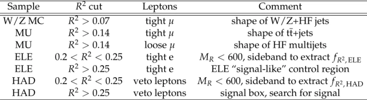
MU box selections with 2b-tagged events, using the sum of two separate exponential terms, as shown in Eq. (5). The fit allows us to obtain a parametric description of the background that is later used in the derivation of the remaining backgrounds, and it also permits the extrapolation of the prediction into the region of higher R and MRvalues. The fit is performed in the region
MR > 400 GeV and is binned in values of R2as shown in Fig. 1. The fit to the simulated data,
which provides a good description of the MRdistribution, is used as the PDF to estimate the
W/Z+b jets background in the signal box.
[GeV] R M 400 600 800 1000 1200 1400 Events / ( 44 GeV ) 1 10 2 10 > 0.07 2 R > 0.14 2 R > 0.20 2 R > 0.30 2 R > 0.38 2 R > 0.50 2 R = 7 TeV s CMS Simulation MU Box
Figure 1: MR distributions for different values of the R2threshold for events passing the MU
box selections in the W/Z+jets MC simulation. The results of the fits (lines) are overlaid with the MRdistributions from the MC simulation (markers).
6.2 tt+jets background estimation
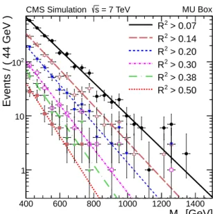
We estimate the tt background from the MU box, using 2b-tagged events in collision data (Sec-tion 4.2) and requiring the presence of a muon passing the tight identifica(Sec-tion requirements (Section 4.1). Based on comparisons with the MC simulation, approximately 90% of the events in this sample are tt. We find empirically from MC simulation studies that the shape of the MR
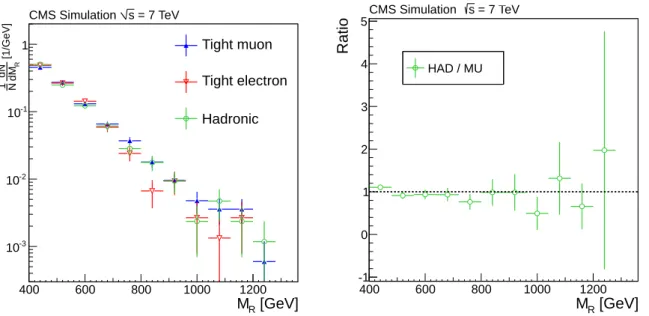
distribution in both the tightly selected MU box and in the HAD box is very similar, as can be seen in Fig. 2. We therefore use the shape derived from the 2b-tagged sample to predict the tt background in the signal region. Additionally, because of a non-negligible contribution of W/Z+HF events in this sample, the imperfections in the W/Z+jets background modeling in the simulation are absorbed into the tt background prediction. In order to derive the tt shape, we constrain the W/Z+jets shape to that obtained from the MC simulation (Section 6.1). We find that a two-exponential function provides a good fit to the observed data in the MU box, as shown in Fig. 3.
6.3 Multijet background
The remaining backgrounds that contribute significantly to the interesting region of high R2 originate from heavy-flavor enriched multijet production. We use events with a loose muon in the MU box to derive the multijets background PDF. According to the MC simulation, this sample is composed 45% of top events, 5% of W/Z+b jet events, and 50% of multijet events.
6.3 Multijet background 9 [GeV] R M 400 600 800 1000 1200 [1/GeV] R dM dN N 1 -3 10 -2 10 -1 10 1 Tight muon Tight electron Hadronic = 7 TeV s CMS Simulation [GeV] R M 400 600 800 1000 1200 Ratio -1 0 1 2 3 4 5 = 7 TeV s CMS Simulation HAD / MU
Figure 2: The MRdistributions (left) in tt MC simulated events selected with either tight MU,
tight ELE and HAD requirements, and (right) the ratio of the number of events selected with the HAD or tight MU selections, as a function of MR.
[GeV] R M 400 600 800 1000 1200 1400 1600 1800 2000 Events / ( 64 GeV ) 1 10 2 10 Observed data Total background + jets t t W/Z + jets = 7 TeV s at -1 CMS 4.8 fb MU Box [GeV] R M 400 600 800 1000 1200 1400 1600 1800 2000 Events / ( 64 GeV ) 1 10 2 10 > 0.14 2 R > 0.20 2 R > 0.30 2 R > 0.38 2 R > 0.50 2 R = 7 TeV s at -1 CMS 4.8 fb MU Box
Figure 3: The result of the fit of the MR distributions (lines) compared to MU box observed
events with R2 >0.14 (left); individual background contributions are not stacked. On the right are shown the MR distributions for different values of the R2 threshold (right) in 2b-tagged
events of the MU box with a tight muon; the results of the fits (lines) are overlaid with the observed distributions (markers).
We proceed to perform the fits, for which the contributions from W/Z+b jets and tt back-grounds are fixed to the PDFs described in Sections 6.1 and 6.2. Based on simulation studies it is found that the parameters of the second component in the fit function (A2and B2in Eq. (5))
are nearly idenical for the multijet and the tt+jets background processes. In order to better con-strain the multijet fit, the parameters of the second component are set equal to those from the
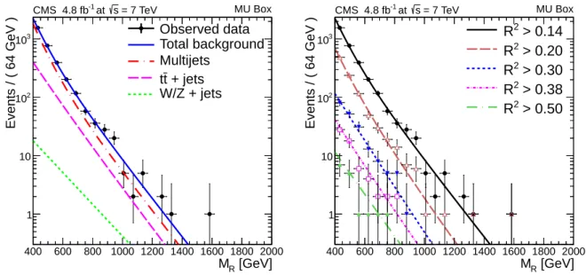
observed events for tt+jets while the parameters of the first component of the multijet PDF are left free. The results of the fit in the 2b-tagged MU box are displayed in Fig. 4, where we find good agreement between the fit results and observed data.
[GeV] R M 400 600 800 1000 1200 1400 1600 1800 2000 Events / ( 64 GeV ) 1 10 2 10 3 10 = 7 TeV s at -1 CMS 4.8 fb MU Box Observed data Total background Multijets + jets t t W/Z + jets [GeV] R M 400 600 800 1000 1200 1400 1600 1800 2000 Events / ( 64 GeV ) 1 10 2 10 3 10 > 0.14 2 R > 0.20 2 R > 0.30 2 R > 0.38 2 R > 0.50 2 R = 7 TeV s at -1 CMS 4.8 fb MU Box
Figure 4: The result of the fit of the MRdistributions (lines) compared to the MU box observed
data for events with R2 >0.14 (left); individual contributions of backgrounds are not stacked. On the right are shown the MR distributions for different values of the R2 threshold (right) in
2b-tagged events of the MU box with a loose muon; the results of the fits (lines) are overlaid with the observed distributions (markers).
6.4 Systematic uncertainties
For the backgrounds estimated from observed events, the uncertainty in the total yield arises from the uncertainties (statistical and systematic) in the fit parameters in Eq. (5). We estimate these uncertainties by varying the R2 threshold values (by ±5%), thus arriving at a new set of Ai and Bi parameters describing the background PDF. The maximum difference observed
between the experimental data and the simulated data in the MU box with tight and loose muon selections is then used as the uncertainty on the shape parameters. This procedure results in a 10% uncertainty in the Aivalues, and 40% in the Bivalues. We also tested the stability of the
fits by varying the initial parameters used to start the fit by±50%, and found that this variation results in stable solutions, returning the same central value for the Aiand Bi parameters.
We generate an ensemble of pseudoexperiments, based on the fit results in the MU box. From each pseudoexperiment a new set of values for the parameters is then obtained, with the corre-sponding uncertainties, and we use the associated PDF results to predict the background yield. The ensemble of pseudoexperiments thus provides a distribution of the expected background yield in the signal regions, with its corresponding uncertainty. This procedure allows us to correctly propagate the systematic uncertainty in the background shape into the prediction of the background. To account for the normalization uncertainty we propagate the uncertainty in the fR2 introduced in Section 5 to the prediction of background yields in the signal region from
control samples in observed events.
The effect of the jet energy scale (JES) and jet energy resolution (JER) uncertainties on the W/Z+jets background estimate and the signal model yields from simulation are taken into
6.5 ELE control region 11
account. These effects are evaluated by repeating the extraction of all background PDFs by first varying the JES/JER by plus or minus one standard deviation in the W/Z+jet background model, and recalculating the E/ and R. These variations correspond to uncertainties as largeT
as 3% in the selection efficiency. We then re-derive the background model PDFs from observed data in the MU box, using the newly obtained W/Z+HF jets model. The new set of PDFs with their corresponding covariance matrices then serve as an alternative background model. We apply a scale factor of about 0.95, that is weakly dependent on jet pT, to account for an
observed difference in tagging efficiency between data and simulation. The uncertainty in the scale factor varies from 0.03 to 0.05 for jets with pTfrom 30 to 670 GeV, and is 0.10 for b jets with
pT > 670 GeV. These uncertainties are measured using a dijet sample with high b-jet purity, as
detailed in Ref. [33].
The uncertainty in the eb1 acceptance due to uncertainties in the parton distribution functions
is calculated using the recommendation from the PDF4LHC group [38]. The parton distri-bution function and the αs variations of next-to-leading (NLO) order in the MSTW2008 [39],
CTEQ6.6 [40], and NNPDF2.0 [41] sets were taken into account and their impact on the signal cross sections was compared with the calculation with CTEQ6L1 [42] that was used in the sim-ulation of the signal samples. From these three sets we evaluate an upper and lower bound on the signal efficiency for each pair of assumed eb1 andχe
0
1 masses, and half of the difference
between the two bounds is used as an estimate of the uncertainty. The theoretical cross section of LQ3production has been calculated using CTEQ6L1 and CTEQ6M [42] at NLO, and the
un-certainty in the prediction of the cross section was estimated by repeating the calculation using the NLO MRST2002 parametrization [43]. This uncertainty was found to vary from 3.5 to 25% for leptoquarks in the mass range considered in this analysis [44].
The systematic uncertainty to the luminosity measurement is taken to be 2.2% [45], which is correlated among all signal channels and the background estimates that are derived from sim-ulations. The uncertainty in trigger efficiency is estimated using a set of prescaled razor triggers with low thresholds, and is found to be 2% for events in the HAD box, and 3% for events in the MU and ELE boxes.
6.5 ELE control region
In order to check that our background shape modeling indeed predicts the observed data ade-quately, we use the PDFs obtained in the steps described above (Sections 6.1-6.3) in an orthog-onal sample in the 2b-tagged ELE box with a tight electron selection, i.e. the sample with a well-identified electron, which is then treated as a neutrino. This signal-depleted sample pro-vides an independent cross-check of our background modeling, and covers the same region in R and MR as the HAD box. Additionally, based on MC simulation studies, the composition
of the tight ELE sample in observed events is similar to that of the HAD sample, consisting of approximately 85% tt, 5% W/Z+HF jets, and 10% multijet events. For comparison, the HAD sample is expected to contain approximately 70%, 5%, and 25% of the respective backgrounds. Using the background model PDFs obtained from the fits, we derive the distribution of the expected shapes in the ELE box using pseudoexperiments. In order to correctly account for correlations and uncertainties in the parameters describing the background model, the shape parameters used to generate each pseudoexperiment data set are sampled from the covariance matrix returned by the fit. The actual number of events in each dataset is then drawn from a Poisson distribution centered on the yield returned by the covariance-matrix sampling. For each pseudoexperiment dataset, the number of events in the sideband and in the high-R2region is found. We then obtain the scale factor fR2, ELE=0.87±0.14 from the sideband region, which
is used to predict the overall yield of background events in the high R2region of the ELE box. The comparison of the predicted MR distribution with the observed events in the ELE box is
shown in Figure 5, and the background model is found to predict the observed data adequately. We also test our ability to correctly predict the yields of SM backgrounds using the scale factor mentioned above. The results are summarized in Table 2. Total background yield in the side-band is normalized to the number of observed data events in the sideside-band, in order to derive the scale factor fR2, ELE, as described in Section 5. The uncertainties in the background yields
shown here represent systematic uncertainties that are estimated by varying the parameters Ai
and Bi, as described in Section 6.4. As can be seen in this comparison, the fR2, ELEobtained from
the sideband allows one to predict the overall normalization of the 2b-tagged sample.
Table 2: Comparison of the yields in the ELE box. The sideband here refers to 2b-tagged events in the ELE box with 400 < MR < 600 GeV and 0.2 < R2 < 0.25, while “signal-like” refers
2b-tagged events with MR > 400 GeV and R > 0.25. The scale factor derived in the sideband
( fR2, ELE=0.87±0.14) is used to normalize the background yield in the signal-like region (third
column), and the uncertainty on the fR2, ELEis propagated into the total background yield.
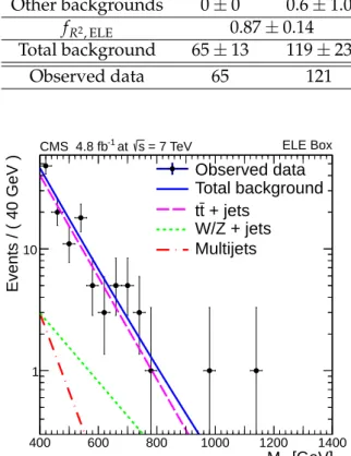
Sideband Signal-like Multijets 12.5±1.9 10±11 W/Z+jets 3.6±1.9 8.8±2.8 tt+jets 58.8±7.7 118.4±9.8 Other backgrounds 0±0 0.6±1.0 fR2, ELE 0.87±0.14 Total background 65±13 119±23 Observed data 65 121 [GeV] R M 400 600 800 1000 1200 1400 Events / ( 40 GeV ) 1 10 Observed data Total background + jets t t W/Z + jets Multijets = 7 TeV s at -1 CMS 4.8 fb ELE Box
Figure 5: The MR distribution for observed data in the 2b-tagged ELE box for events with
R2 > 0.25 compared to the prediction. The background model derived from the MU box is
used to predict the MR shapes of the background processes. The individual contributions are
not stacked.
We perform another check to test whether the R2-dependence is well-described by our back-ground model. This check is needed since in the final signal region we have several signal
13
boxes, each optimized for different signal mass hypotheses. In order to increase the sensitivity for higher masses, a tighter selection on R2is imposed to reduce the backgrounds further, while keeping the signal efficiency high. In order to ensure that our background model adequately describes observed data with higher R2thresholds, we perform the same procedure in the ELE
box. The results are summarized in Table 3. Here, we use the same fR2, ELEderived from the
sideband. As can be seen from these results, this model correctly predicts the total yields for higher R2boxes.
Table 3: Expected and observed yields in the 2b-tagged ELE box for R2selections and a fixed
re-quirement MR>400 GeV. The quoted uncertainties on the expected number of events include
statistical and systematic uncertainties, and the uncertainty on the scale factor fR2, ELE.
R2Cut Expected yields Observed yields
>0.25 119±23 121 0.25–0.30 51±17 48 0.30–0.35 30±10 26 0.35–0.38 9.9±5.2 11 0.38–0.42 11.5±5.0 11 >0.42 16.8±4.8 25
7
Results
We search for LQ3 and eb1 signals in the HAD box data sample using the background PDFs
obtained from the MU box (Sections 6.1-6.3). The predicted background yields and their un-certainties are summarized in Table 4. Total background yield in the 2b-tagged sideband is normalized to the number of observed data events in the sideband, in order to derive the scale factor fR2, HAD =1.10±0.13, as described in Section 5. The distributions of R and MRobserved
in the 2b-tagged HAD box are compared to the background prediction in Fig. 6.
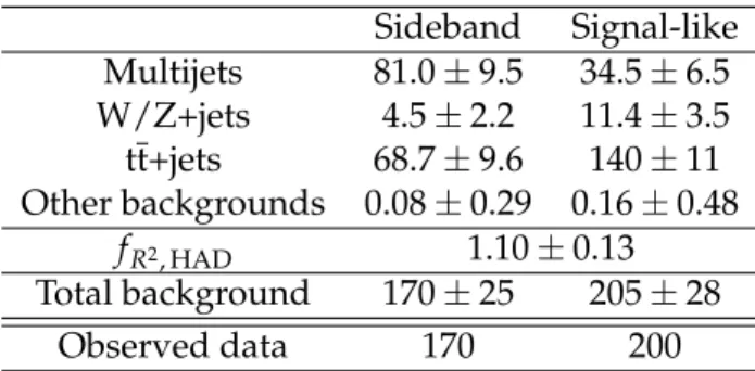
Table 4: Comparison of the yields in the 2b-tagged (signal region) samples in the HAD box. The uncertainties include the systematic uncertainty in the background shapes (Section 6.4) and statistical uncertainties. The uncertainty in the total yield after scaling also includes the jet energy scale uncertainty. The scale factor derived in the sideband ( fR2, HAD = 1.10±0.13) is
used to normalize the background yield in the signal-like region. The uncertainty in fR2, HAD is
propagated and included in the quoted uncertainty in the expected background yields. Sideband Signal-like Multijets 81.0±9.5 34.5±6.5 W/Z+jets 4.5±2.2 11.4±3.5 tt+jets 68.7±9.6 140±11 Other backgrounds 0.08±0.29 0.16±0.48 fR2, HAD 1.10±0.13 Total background 170±25 205±28 Observed data 170 200
As seen in Fig. 6 and Table 4, both the number of observed events and the shapes of the R and MRdistributions are in agreement with the expected SM backgrounds. Therefore, we proceed
to define two signal regions, to enhance the sensitivity for different LQ3 masses. The regions
[GeV] R M 400 600 800 1000 1200 1400 Events / ( 40 GeV ) 1 10 2 10 Observed data Multijets W/Z + jets + jets t t = 350 GeV) 3 LQ (M 3 Background + LQ (550 GeV) 3 LQ Signal 1 b ~ = 100 GeV) 0 1 χ∼ = 300 GeV, M 1 b ~ (M = 7 TeV s at -1 CMS 4.7 fb HAD Box 2 R 0.25 0.3 0.35 0.4 0.45 0.5 Events 0 20 40 60 80 100 120 140 160 180 Observed data Background = 350 GeV) 3 LQ (M 3 Background + LQ Signal 1 b ~ = 100 GeV) 0 1 χ∼ = 300 GeV, M 1 b ~ (M Background Uncertainty = 7 TeV s at -1 CMS 4.7 fb HAD Box
Figure 6: Comparison of the background prediction with the data observed in the 2b-tagged sample in the HAD signal box for the MR(left) and R (right) distributions. The expected
con-tributions from LQ3and eb1signal events with various mass hypotheses are also shown.
on R and MR. We find that MR > 400 GeV provides the best sensitivity for all masses, and
for LQ3 masses below 350 GeV the optimal selection is R2 > 0.25, while for higher masses
R2 > 0.42 provides best sensitivity. Because of the high value assumed for the χe
0
1 mass in
the eb1search, the inclusive selection of MR > 400 GeV and R2 > 0.25 is found to provide the
optimal sensitivity in the mass range considered in this analysis.
Table 5 shows the comparison of the expected background yields in these signal boxes, and agreement of the observed event counts with the expectations is observed. Table 6 shows the efficiency of these selections for several LQ3mass hypotheses, based on MC simulation.
Effi-ciencies for the eb1signal are shown in Fig. 7. Typical efficiencies range from a few percent up to
∼12 percent for eb1 masses between 200 and 500 GeV and smallχe
0
1 mass. The efficiency drops
when the mass of the eb1squark is close to the mass ofχe
0
1, since the resulting b jets are softer in
these scenarios.
Table 5: Expected and observed yields in the 2b-tagged HAD box for various R2selections and a fixed MR>400 GeV requirement. The quoted uncertainties on the expected number of events
include statistical and systematic uncertainties, and the uncertainty from the fR2, HAD. The left
three columns show inclusive yields above the R2 threshold, while the right three columns show the yields in bins of R2.
R2Cut Expected yields Observed yields R2bins Expected yields Observed yields
>0.25 205±28 200 0.25–0.30 105±25 97
>0.30 100±16 103 0.30–0.35 44±11 49
>0.35 56±12 54 0.35–0.38 13±9 14
>0.38 43±9 40 0.38–0.42 18±6 13
>0.42 25±7 27 >0.42 25±7 27
ex-15
Table 6: Summary of the expected LQ3 signal yields and efficiency in the signal region, for
4.7 fb−1of observed data, in events with MR >400 GeV. For LQ3masses below 350 GeV R2 >
0.25 is required, while for heavier masses we require events to pass R2>0.42. All uncertainties are statistical only.
MLQ3 [GeV] σ(pb) Efficiency (%) Number of expected events 200 12 0.33 185±13 250 3.5 1.1 171.2±9.1 280 1.8 1.8 151.4±3.6 320 0.82 3.2 122.8±1.9 350 0.48 1.8 39.2±1.3 450 0.095 4.3 19.17±0.38 550 0.024 5.9 6.59±0.12 [GeV] 1 b ~ M 50 100 150 200 250 300 350 400 450 500
[GeV]
0 1 χ∼M
50 100 150 200 250 300 350 400 450 500 0 0.02 0.04 0.06 0.08 0.1 0.12 = 7 TeV s CMS Simulation 1% 5% 10%Figure 7: Signal efficiency for simulated eb1 signal events with MR > 400 GeV and R2 > 0.25.
White lines show the iso-efficiency contours for 1, 5, and 10% signal efficiency, respectively. pected value equal to the sum of the signal and expected backgrounds. Log-normal priors for the nuisance parameters are used to model the systematic uncertainties listed in Section 6.4. A 95% CL upper limit is set on the potential signal cross section, as summarized in Table 7. The modified frequentist construction CLs[46, 47] is used for limit calculation. These limits are
interpreted in terms of limits of LQ3pair production cross section as shown in Fig. 8. The upper
limits are compared to the NLO prediction of the LQ pair production cross section [44], and we set a 95% CL exclusion on LQ masses smaller than 440 GeV (expected 470 GeV), assuming β=0. We also present the 95% CL limit on β as a function of LQ3mass as shown on the right
side of Fig. 8.
The results of the analysis are interpreted in the context of the simplified supersymmetry model spectra (SMS) [48–50]. In SMS, a limited set of hypothetical particles and decay chains are
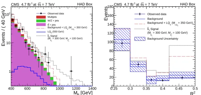
intro-Table 7: Observed and expected 95% CL upper limits on the LQ3pair-production cross section
as a function of the LQ3mass.
MLQ3 [GeV] -2σ -1σ Median expected limit [pb] +1σ +2σ Observed limit [pb] 200 2.0 3.3 4.5 6.2 8.4 4.3 250 0.64 1.1 1.4 2.0 2.6 1.3 270 0.43 0.75 0.97 1.4 1.8 0.90 330 0.18 0.24 0.33 0.46 0.62 0.36 350 0.13 0.17 0.23 0.32 0.42 0.25 450 0.047 0.067 0.092 0.13 0.17 0.10 550 0.037 0.049 0.066 0.094 0.13 0.073 [GeV] 3 LQ M 200 250 300 350 400 450 500 550 [pb] 2 ) β (1-× +X) 3 LQ 3 LQ → (pp σ -2 10 -1 10 1 10 σ Expected 1 σ Expected 2 Observed limit Theory ) -1 D0 exclusion (5.2 fb = 7 TeV s at -1 CMS 4.7 fb [GeV] 3 LQ M 200 250 300 350 400 450 β 1 - 0.3 0.4 0.5 0.6 0.7 0.8 0.9 1 ) -1 D0 exclusion (5.2 fb ) -1 CMS 95% CL Limit (observed, 4.7 fb ) -1 CMS 95% CL Limit (expected, 4.7 fb = 7 TeV s at -1 CMS 4.7 fb
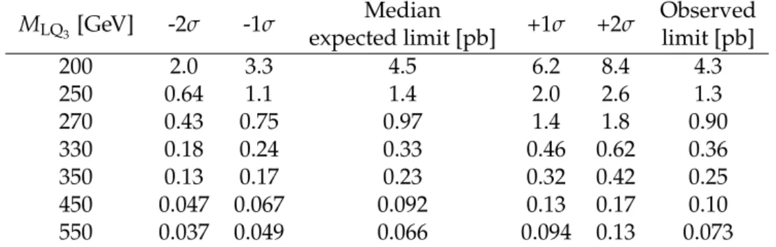
Figure 8: (Left) the expected and observed upper limit at 95% CL on the LQ3 pair production
cross section as a function of the LQ3 mass, assuming β = 0. The systematic uncertainties
reported in Section 6.4 are included in the calculation. The vertical greyed region is excluded by the current D0 limit [12] in the same channel. The theory curve and its band represent, respectively, the theoretical LQ3pair production cross section and the uncertainties due to the
choice of parton distribution functions and renormalization/factorization scales [44]. (Right) minimum β for a 95% CL exclusion of the LQ3 hypothesis as a function of LQ3 mass. The
observed (expected) exclusion curve is obtained using the observed (expected) upper limit and the central value of the theoretical LQ3 pair production cross section. The band around the
observed exclusion curve is obtained by considering the observed upper limit while taking into account the uncertainties on the theoretical cross section. The grey region is excluded by the current D0 limits [12] in the same channel.
duced to produce a given topological signature, such as the E/ plus b jets final state consideredT
in this analysis. We consider a SMS scenario where all supersymmetric particles are set to have a very large mass, except for the eb1andχe
0
1. The pairs of scalar bottom quarks produced
through strong interactions are kinematically allowed to decay only into a b quark and aχe
0 1.
The observed and expected 95% CL upper limits in the ˜b1−χe
0
17 [GeV] 1 b ~ M 100 150 200 250 300 350 400 450 500 550 [GeV]0χ∼1 M 60 80 100 120 140 160 180 200 220 240 forbidden 0 1 χ ∼ b → 1 b ~ (th.)) σ 1 ± Observed Limit ( (exp.)) σ 1 ± Expected Limit ( -1 CDF 2.65 fb -1 D0 5.2 fb ) q ~ ) >> m( g ~ ; m( 0 1 χ∼ b → 1 b ~ = 7 TeV s at -1 CMS 4.7 fb
Figure 9: The expected and observed 95% CL exclusion limits for the eb1pair production SMS
model. The red dashed contour shows the 95% CL exclusion limits based on the NLO+NLL cross section. The red dotted contours represent the theoretical uncertainties from the variation of parton distribution functions, and renormalization and factorization scales. The correspond-ing expected limits are shown with the black dashed contour. The shaded yellow contours represent the uncertainties in the SM background estimates, as reported in Section 6.4.
Fig. 9, where the eb1pair production cross section is calculated at the NLO and
next-to-leading-logarithm (NLL) order [51–56]. Since MRdepends on the squared difference of the masses of eb1
andχe
0
1, at the eb1masses around 400-450 GeV and lowχe
0
1 masses the exclusion limit is almost
independent of the χe
0
1 mass. The signal acceptance in the region with small mass splitting
between the eb1 andχe
0
1 is particularly susceptible to uncertainties associated with initial-state
radiation (ISR). The impact of ISR is estimated by comparing the results of the acceptance cal-culation using PYTHIA with the “power shower” and with moderate ISR settings [19]. If the acceptance varies by more than 25% for a particular choice of eb1andχe
0
1 masses, then no limit
is set for those mass parameters. This procedure results in reduced sensitivity in the region of m(eb1) < 300 GeV and 80 < m(χe01) < 130 GeV, and thus an inability to exclude some of the models in this parameter range.
8
Summary
A search has been performed for third-generation scalar leptoquarks and for scalar bottom quarks in the all-hadronic channel with a signature of large E/ and b-tagged jets. This searchT
is based on a data sample collected in pp collisions at√s = 7 TeV and corresponding to an integrated luminosity of 4.7 fb−1. The number of observed events is in agreement with the predictions for the SM backgrounds. We set an upper limit on the LQ3 pair production cross
section, excluding a scalar LQ3with mass below 450 GeV, assuming a 100% branching fraction
of the LQ3to b quarks and tau neutrinos. We set 95% confidence level upper limits in the ˜b1−χe
0 1
mass plane such that for neutralino masses of 50 GeV, scalar bottom masses up to 410 GeV are excluded. These results represent the most stringent limits on LQ3masses and extend limits on
e
b1masses to much higher values than probed previously.
Acknowledgements
We congratulate our colleagues in the CERN accelerator departments for the excellent perfor-mance of the LHC machine. We thank the technical and administrative staff at CERN and other CMS institutes, and acknowledge support from BMWF and FWF (Austria); FNRS and FWO (Belgium); CNPq, CAPES, FAPERJ, and FAPESP (Brazil); MEYS (Bulgaria); CERN; CAS, MoST, and NSFC (China); COLCIENCIAS (Colombia); MSES (Croatia); RPF (Cyprus); MoER, SF0690030s09 and ERDF (Estonia); Academy of Finland, MEC, and HIP (Finland); CEA and CNRS/IN2P3 (France); BMBF, DFG, and HGF (Germany); GSRT (Greece); OTKA and NKTH (Hungary); DAE and DST (India); IPM (Iran); SFI (Ireland); INFN (Italy); NRF and WCU (Ko-rea); LAS (Lithuania); CINVESTAV, CONACYT, SEP, and UASLP-FAI (Mexico); MSI (New Zealand); PAEC (Pakistan); MSHE and NSC (Poland); FCT (Portugal); JINR (Armenia, Be-larus, Georgia, Ukraine, Uzbekistan); MON, RosAtom, RAS and RFBR (Russia); MSTD (Ser-bia); SEIDI and CPAN (Spain); Swiss Funding Agencies (Switzerland); NSC (Taipei); ThEP, IPST and NECTEC (Thailand); TUBITAK and TAEK (Turkey); NASU (Ukraine); STFC (United Kingdom); DOE and NSF (USA). Individuals have received support from the Marie-Curie programme and the European Research Council (European Union); the Leventis Foundation; the A. P. Sloan Foundation; the Alexander von Humboldt Foundation; the Belgian Federal Science Policy Office; the Fonds pour la Formation `a la Recherche dans l’Industrie et dans l’Agriculture (FRIA-Belgium); the Agentschap voor Innovatie door Wetenschap en Technolo-gie (IWT-Belgium); the Ministry of Education, Youth and Sports (MEYS) of Czech Republic; the Council of Science and Industrial Research, India; the Compagnia di San Paolo (Torino); and the HOMING PLUS programme of Foundation for Polish Science, cofinanced from European Union, Regional Development Fund.
References
[1] J. C. Pati and A. Salam, “Lepton number as the fourth ‘color”’, Phys. Rev. D 10 (1974) 275, doi:10.1103/PhysRevD.10.275.
[2] B. Schrempp and F. Schrempp, “Light leptoquarks”, Phys. Lett. B 153 (1985) 101, doi:10.1016/0370-2693(85)91450-9.
[3] B. Gripaios et al., “Searching for third-generation composite leptoquarks at the LHC”, J. High Energy Phys. 01 (2011) 156, doi:10.1007/JHEP01(2011)156,
arXiv:1010.3962.
[4] S. Dimopoulos and L. Susskind, “Mass without scalars”, Nucl. Phys. B 155 (1979) 237, doi:10.1016/0550-3213(79)90364-X.
[5] S. Dimopoulos, “Technicoloured signatures”, Nucl. Phys. B 168 (1980) 69, doi:10.1016/0550-3213(80)90277-1.
[6] E. Farhi and L. Susskind, “Technicolour”, Phys. Rep. 74 (1981) 277, doi:10.1016/0370-1573(81)90173-3.
[7] J. L. Hewett and T. G. Rizzo, “Low-energy phenomenology of superstring-inspired E6
References 19
[8] S. Davidson, D. C. Bailey, and B. A. Campbell, “Model independent constraints on leptoquarks from rare processes”, Z. Phys. C 61 (1994) 613,
doi:10.1007/BF01552629, arXiv:hep-ph/9309310.
[9] G. R. Farrar and P. Fayet, “Phenomenology of the production, decay, and detection of new hadronic states associated with supersymmetry”, Phys. Lett. B 76 (1978) 575, doi:10.1016/0370-2693(78)90858-4.
[10] J. L. Feng, “Dark matter candidates from particle physics and methods of detection”, Annu. Rev. Astron. Astr. 48 (2010) 495,
doi:10.1146/annurev-astro-082708-101659.
[11] S. Dimopoulos and G. F. Giudice, “Naturalness constraints in supersymmetric theories with non-universal soft terms”, Phys. Lett. B 357 (1995) 573,
doi:10.1016/0370-2693(95)00961-J.
[12] D0 Collaboration, “Search for scalar bottom quarks and third-generation leptoquarks in p¯p collisions at√s=1.96 TeV”, Phys. Lett. B 693 (2010) 95,
doi:10.1016/j.physletb.2010.08.028.
[13] CDF Collaboration, “Search for the production of scalar bottom quarks in pp collisions at√ s =1.96 TeV”, Phys. Rev. Lett. 105 (2010) 081802,
doi:10.1103/PhysRevLett.105.081802.
[14] CMS Collaboration, “Search for pair production of third generation leptoquarks and stops that decay to a tau and a b quark”, (2012). arXiv:1210.5629.
[15] ATLAS Collaboration, “Search for scalar bottom quark pair production with the ATLAS detector in pp collisions at√s=7 TeV”, Phys. Rev. Lett. 108 (2012) 181802,
doi:10.1103/PhysRevLett.108.181802.
[16] CMS Collaboration, “The CMS experiment at the CERN LHC”, J. Instrum. 3 (2008) S08004, doi:10.1088/1748-0221/3/08/S08004.
[17] C. Rogan, “Kinematics for new dynamics at the LHC”, (2010). arXiv:1006.2727. [18] CMS Collaboration, “Inclusive search for squarks and gluinos in pp collisions at√
s =7 TeV”, Phys. Rev. D 85 (2011) 012004, doi:10.1103/PhysRevD.85.012004. [19] T. Sj ¨ostrand, S. Mrenna, and P. Z. Skands, “PYTHIA6.4 physics and manual”, J. High
Energy Phys. 05 (2006) 026, doi:10.1088/1126-6708/2006/05/026.
[20] J. Alwall et al., “MADGRAPH5 : going beyond”, J. High Energy Phys. 06 (2011) 128, doi:10.1007/JHEP06(2011)128.
[21] GEANT4 Collaboration, “GEANT4—a simulation toolkit”, Nucl. Instrum. Meth. A 506 (2003) 250, doi:10.1016/S0168-9002(03)01368-8.
[22] CMS Collaboration, “Measurement of the underlying event activity at the LHC with√ s =7 TeV and comparison with√s =0.9 TeV”, J. High Energy Phys. 09 (2011) 109, doi:10.1007/JHEP09(2011)109.
[24] R. Field, “Studying the underlying event at CDF and the LHC”, in Proceedings of the First International Workshop on Multiple Partonic Interactions at the LHC MPI’08, October 27-31, 2008, P. Bartalini and L. Fan ´o, eds., p. 12. October, 2009. arXiv:1003.4220.
[25] CMS Collaboration, “Comparison of the fast simulation of CMS with the first LHC data”, CMS Detector Performance Summary CMS-DP-2010-039, (2010).
[26] CMS Collaboration, “Tracking and Primary Vertex Results in First 7 TeV Collisions”, CMS Physics Analysis Summary CMS-PAS-TRK-10-005, (2010).
[27] CMS Collaboration, “Missing transverse energy performance of the CMS detector”, J. Instrum. 6 (2011) P09001, doi:10.1088/1748-0221/6/09/P09001.
[28] M. Cacciari, G. P. Salam, and G. Soyez, “The anti-ktjet clustering algorithm”, J. High
Energy Phys. 04 (2008) 063, doi:10.1088/1126-6708/2008/04/063.
[29] CMS Collaboration, “Determination of jet energy calibration and transverse momentum resolution in CMS”, J. Instrum. 6 (2011) P11002,
doi:10.1088/1748-0221/6/11/P11002.
[30] CMS Collaboration, “Commissioning of the Particle-Flow Reconstruction in Minimum-Bias and Jet Events from pp Collisions at 7 TeV”, CMS Physics Analysis Summary CMS-PAS-PFT-10-002, (2010).
[31] CMS Collaboration, “Measurements of inclusive W and Z cross sections in pp collisions at√s=7 TeV”, J. High Energy Phys. 01 (2011) 080, doi:10.1007/JHEP01(2011)080. [32] M. Cacciari and G. P. Salam, “Pileup subtraction using jet areas”, Phys. Lett. B 659 (2008)
119, doi:10.1016/j.physletb.2007.09.077.
[33] CMS Collaboration, “b-Jet Identification in the CMS Experiment”, CMS Physics Analysis Summary CMS-PAS-BTV-11-004, (2011).
[34] CMS Collaboration, “Measurement of the t¯t production cross section and the top quark mass in the dilepton channel in pp collisions at√s =7 TeV”, J. High Energy Phys. 07 (2011) 049, doi:10.1007/JHEP07(2011)049.
[35] W. Verkerke and D. Kirkby, “The ROOFITtoolkit for data modeling”, (2003). arXiv:physics/0306116.
[36] CMS Collaboration, “Study of the dijet invariant mass distribution in W→ `νplus jets events produced in pp collisions at√s =7 TeV”, CMS Physics Analysis Summary CMS-PAS-EWK-11-017, (2011).
[37] CMS Collaboration, “Measurement of the Z/gamma*+b-jet cross section in pp collisions at 7 TeV”, J. High Energy Phys. 06 (2012) 126, doi:10.1007/JHEP06(2012)126. [38] M. Botje et al., “The PDF4LHC working group interim recommendations”, (2011).
arXiv:1101.0538.
[39] A. D. Martin et al., “Parton distributions for the LHC”, Eur. Phys. J. C 63 (2009) 189, doi:10.1140/epjc/s10052-009-1072-5.
[40] P. M. Nadolsky et al., “Implications of CTEQ global analysis for collider observables”, Phys. Rev. D 78 (2008) 013004, doi:10.1103/PhysRevD.78.013004.
References 21
[41] R. D. Ball et al., “A first unbiased global NLO determination of parton distributions and their uncertainties”, Nucl. Phys. B 838 (2010) 136,
doi:10.1016/j.nuclphysb.2010.05.008.
[42] J. Pumplin et al., “New generation of parton distributions with uncertainties from global QCD analysis”, J. High Energy Phys. 07 (2002) 012,
doi:10.1088/1126-6708/2002/07/012, arXiv:hep-ph/0201195. [43] A. D. Martin et al., “Uncertainties of predictions from parton distributions I:
Experimental errors”, Eur. Phys. J. C 28 (2003) 455, doi:10.1140/epjc/s2003-01196-2.
[44] M. Kr¨amer et al., “Pair production of scalar leptoquarks at the LHC”, Phys. Rev. D 71 (2005) 057503, doi:10.1103/PhysRevD.71.057503.
[45] CMS Collaboration, “Absolute Calibration of the Luminosity Measurement at CMS: Winter 2012 Update”, CMS Physics Analysis Summary CMS-PAS-SMP-12-008, (2012). [46] A. L. Read, “Presentation of search results: the CLstechnique”, J. Phys. G 28 (2002) 2693,
doi:10.1088/0954-3899/28/10/313.
[47] T. Junk, “Confidence level computation for combining searches with small statistics”, Nucl. Instrum. Meth. A 434 (1999) 435, doi:10.1016/S0168-9002(99)00498-2. [48] D. Alves et al., “Simplified models for LHC new physics searches”, (2011).
arXiv:1105.2838.
[49] J. Alwall, P. Schuster, and N. Toro, “Simplified models for a first characterization of new physics at the LHC”, Phys. Rev. D 79 (2009) 075020,
doi:10.1103/PhysRevD.79.075020.
[50] J. Alwall et al., “Model-independent jets plus missing energy searches”, Phys. Rev. D 79 (2009) 015005, doi:10.1103/PhysRevD.79.015005.
[51] W. Beenakker et al., “Squark and gluino production at hadron colliders”, Nucl. Phys. B
492(1997) 51, doi:10.1016/S0550-3213(97)00084-9.
[52] A. Kulesza and L. Motyka, “Threshold resummation for squark-antisquark and gluino-pair production at the LHC”, Phys. Rev. Lett. 102 (2009) 111802,
doi:10.1103/PhysRevLett.102.111802.
[53] A. Kulesza and L. Motyka, “Soft gluon resummation for the production of gluino-gluino and squark-antisquark pairs at the LHC”, Phys. Rev. D 80 (2009) 095004,
doi:10.1103/PhysRevD.80.095004.
[54] W. Beenakker et al., “Soft-gluon resummation for squark and gluino hadroproduction”, J. High Energy Phys. 0912 (2009) 041, doi:10.1088/1126-6708/2009/12/041. [55] W. Beenakker et al., “Squark and gluino hadroproduction”, Int. J. Mod. Phys. A 26 (2011)
2637, doi:10.1142/S0217751X11053560.
[56] M. Kr¨amer et al., “Supersymmetry production cross sections in pp collisions at√ s =7 TeV”, (2012). arXiv:1206.2892.
23
A
The CMS Collaboration
Yerevan Physics Institute, Yerevan, Armenia
S. Chatrchyan, V. Khachatryan, A.M. Sirunyan, A. Tumasyan
Institut f ¨ur Hochenergiephysik der OeAW, Wien, Austria
W. Adam, E. Aguilo, T. Bergauer, M. Dragicevic, J. Er ¨o, C. Fabjan1, M. Friedl, R. Fr ¨uhwirth1, V.M. Ghete, N. H ¨ormann, J. Hrubec, M. Jeitler1, W. Kiesenhofer, V. Kn ¨unz, M. Krammer1, I. Kr¨atschmer, D. Liko, I. Mikulec, M. Pernicka†, D. Rabady2, B. Rahbaran, C. Rohringer,
H. Rohringer, R. Sch ¨ofbeck, J. Strauss, A. Taurok, W. Waltenberger, C.-E. Wulz1
National Centre for Particle and High Energy Physics, Minsk, Belarus
V. Mossolov, N. Shumeiko, J. Suarez Gonzalez
Universiteit Antwerpen, Antwerpen, Belgium
M. Bansal, S. Bansal, T. Cornelis, E.A. De Wolf, X. Janssen, S. Luyckx, L. Mucibello, S. Ochesanu, B. Roland, R. Rougny, M. Selvaggi, H. Van Haevermaet, P. Van Mechelen, N. Van Remortel, A. Van Spilbeeck
Vrije Universiteit Brussel, Brussel, Belgium
F. Blekman, S. Blyweert, J. D’Hondt, R. Gonzalez Suarez, A. Kalogeropoulos, M. Maes, A. Olbrechts, S. Tavernier, W. Van Doninck, P. Van Mulders, G.P. Van Onsem, I. Villella
Universit´e Libre de Bruxelles, Bruxelles, Belgium
B. Clerbaux, G. De Lentdecker, V. Dero, A.P.R. Gay, T. Hreus, A. L´eonard, P.E. Marage, A. Mohammadi, T. Reis, L. Thomas, C. Vander Velde, P. Vanlaer, J. Wang
Ghent University, Ghent, Belgium
V. Adler, K. Beernaert, A. Cimmino, S. Costantini, G. Garcia, M. Grunewald, B. Klein, J. Lellouch, A. Marinov, J. Mccartin, A.A. Ocampo Rios, D. Ryckbosch, M. Sigamani, N. Strobbe, F. Thyssen, M. Tytgat, S. Walsh, E. Yazgan, N. Zaganidis
Universit´e Catholique de Louvain, Louvain-la-Neuve, Belgium
S. Basegmez, G. Bruno, R. Castello, L. Ceard, C. Delaere, T. du Pree, D. Favart, L. Forthomme, A. Giammanco3, J. Hollar, V. Lemaitre, J. Liao, O. Militaru, C. Nuttens, D. Pagano, A. Pin, K. Piotrzkowski, J.M. Vizan Garcia
Universit´e de Mons, Mons, Belgium
N. Beliy, T. Caebergs, E. Daubie, G.H. Hammad
Centro Brasileiro de Pesquisas Fisicas, Rio de Janeiro, Brazil
G.A. Alves, M. Correa Martins Junior, T. Martins, M.E. Pol, M.H.G. Souza
Universidade do Estado do Rio de Janeiro, Rio de Janeiro, Brazil
W.L. Ald´a J ´unior, W. Carvalho, A. Cust ´odio, E.M. Da Costa, D. De Jesus Damiao, C. De Oliveira Martins, S. Fonseca De Souza, H. Malbouisson, M. Malek, D. Matos Figueiredo, L. Mundim, H. Nogima, W.L. Prado Da Silva, A. Santoro, L. Soares Jorge, A. Sznajder, A. Vilela Pereira
Instituto de Fisica Teorica, Universidade Estadual Paulista, Sao Paulo, Brazil
T.S. Anjos4, C.A. Bernardes4, F.A. Dias5, T.R. Fernandez Perez Tomei, E.M. Gregores4, C. Lagana, F. Marinho, P.G. Mercadante4, S.F. Novaes, Sandra S. Padula
Institute for Nuclear Research and Nuclear Energy, Sofia, Bulgaria
V. Genchev2, P. Iaydjiev2, S. Piperov, M. Rodozov, S. Stoykova, G. Sultanov, V. Tcholakov, R. Trayanov, M. Vutova
University of Sofia, Sofia, Bulgaria
A. Dimitrov, R. Hadjiiska, V. Kozhuharov, L. Litov, B. Pavlov, P. Petkov
Institute of High Energy Physics, Beijing, China
J.G. Bian, G.M. Chen, H.S. Chen, C.H. Jiang, D. Liang, S. Liang, X. Meng, J. Tao, J. Wang, X. Wang, Z. Wang, H. Xiao, M. Xu, J. Zang, Z. Zhang
State Key Lab. of Nucl. Phys. and Tech., Peking University, Beijing, China
C. Asawatangtrakuldee, Y. Ban, Y. Guo, W. Li, S. Liu, Y. Mao, S.J. Qian, H. Teng, D. Wang, L. Zhang, W. Zou
Universidad de Los Andes, Bogota, Colombia
C. Avila, C.A. Carrillo Montoya, J.P. Gomez, B. Gomez Moreno, A.F. Osorio Oliveros, J.C. Sanabria
Technical University of Split, Split, Croatia
N. Godinovic, D. Lelas, R. Plestina6, D. Polic, I. Puljak2
University of Split, Split, Croatia
Z. Antunovic, M. Kovac
Institute Rudjer Boskovic, Zagreb, Croatia
V. Brigljevic, S. Duric, K. Kadija, J. Luetic, D. Mekterovic, S. Morovic
University of Cyprus, Nicosia, Cyprus
A. Attikis, M. Galanti, G. Mavromanolakis, J. Mousa, C. Nicolaou, F. Ptochos, P.A. Razis
Charles University, Prague, Czech Republic
M. Finger, M. Finger Jr.
Academy of Scientific Research and Technology of the Arab Republic of Egypt, Egyptian Network of High Energy Physics, Cairo, Egypt
Y. Assran7, S. Elgammal8, A. Ellithi Kamel9, A.M. Kuotb Awad10, M.A. Mahmoud10, A. Radi11,12
National Institute of Chemical Physics and Biophysics, Tallinn, Estonia
M. Kadastik, M. M ¨untel, M. Murumaa, M. Raidal, L. Rebane, A. Tiko
Department of Physics, University of Helsinki, Helsinki, Finland
P. Eerola, G. Fedi, M. Voutilainen
Helsinki Institute of Physics, Helsinki, Finland
J. H¨ark ¨onen, A. Heikkinen, V. Karim¨aki, R. Kinnunen, M.J. Kortelainen, T. Lamp´en, K. Lassila-Perini, S. Lehti, T. Lind´en, P. Luukka, T. M¨aenp¨a¨a, T. Peltola, E. Tuominen, J. Tuominiemi, E. Tuovinen, D. Ungaro, L. Wendland
Lappeenranta University of Technology, Lappeenranta, Finland
K. Banzuzi, A. Karjalainen, A. Korpela, T. Tuuva
DSM/IRFU, CEA/Saclay, Gif-sur-Yvette, France
M. Besancon, S. Choudhury, M. Dejardin, D. Denegri, B. Fabbro, J.L. Faure, F. Ferri, S. Ganjour, A. Givernaud, P. Gras, G. Hamel de Monchenault, P. Jarry, E. Locci, J. Malcles, L. Millischer, A. Nayak, J. Rander, A. Rosowsky, M. Titov
Laboratoire Leprince-Ringuet, Ecole Polytechnique, IN2P3-CNRS, Palaiseau, France
S. Baffioni, F. Beaudette, L. Benhabib, L. Bianchini, M. Bluj13, P. Busson, C. Charlot, N. Daci, T. Dahms, M. Dalchenko, L. Dobrzynski, A. Florent, R. Granier de Cassagnac, M. Haguenauer,