Combining Statistical Methodologies in Water
Quality Monitoring in a Hydrological Basin –
Space and Time Approaches
Marco Costa
1and A. Manuela Gonçalves
21
CMAF and Escola Superior de Tecnologia e Gestão de Águeda, Universidade de Aveiro,
2
CMAT and Departamento de Matemática e Aplicações, Universidade do Minho,
Portugal
1. Introduction
As water is a precious asset as well as a potential inducer of riches, water quality monitoring networks are important tools in the management and assessment of surface water quality and they could be improved by means of accurate forecasts of surface water variables. The administration of hydrologic resources has been deserving a special prominence in the context of domestic and international politics in order to solve the complexity and uncertainty of the problems associated with a worldwide and local scale of sustainable administration (environmental, social, and economical) of natural water resources. Directive 2000/60/CE (UE 2000) of the European Parliament and Council (Water Framework Directive - WFD) establishing a framework for the community action in the field of water policy was incorporated into the domestic legislation in 2005 by Law nr 58/2005 and by Decree-Law nr 77/2006. According to this Directive, each member-state has to project, improve and recover all surface waters in order to achieve a good qualitative and quantitative status of all water bodies by 2015 (Machado et al., 2010). The relevance and interest that these subjects have been raising, specially in the Portuguese community, originated an entire group of state strategies and a new legal framework (INAG, 2008a, 2008b) derived from the WFD.
The river basin, which is the primordial unity of water resources planning and management, is usually submitted to pressures and changes due to human activities. Each hydrological basin is unique because it is a system that comprises orographic properties, ecological status, natural and anthropogenic factors, and where a network of water monitoring sites and a network of meteorological stations are integrated, thus allowing a correct monitoring of water quality.
At a river basin scale there is a need to establish a methodology for systematic data monitoring, characterization of surface water quality and a correct analysis of collected data (Vega et al., 1998). Surface water quality monitoring has as its main objective the characterization of water resources, as well as the monitoring of its space-time evolution in order to achieve an appropriate administration.
W
ater quality monitoring is an area encompassing a large set of disciplines. Statistical methodologies have been applied and developed with a particular emphasis on the last decades. Usually, data sets of environmental issues, namely of water quality measurements, have a significant complexity because they may have different properties simultaneously, and this implies a high level of tight, multi-disciplinary connection between water management technical bodies and instruments of analysis for decision-making (Vieira, 2003).Multivariate statistical analyses have become widely applied in water quality assessment and sources apportionment of water over the last years (Wunderlin et al., 2001; Simeonov et al., 2003; Shrestha & Kazama, 2007). In several works, multivariate statistical analyses are applied to sets of water quality variables, usually comprised of quantitative analytical data. If the goal is to investigate the evaluation of water quality temporal or spatial variations as in Helena et al. (2000) or the natural and anthropogenic origin of contaminants in surface or ground water, as in Ato et al. (2010), the most suitable and applied approach is the principal components analysis (Liu et al., 2003; Lischeid, 2009; Varol & Sen, 2009). In some practical studies, there is data from a group of sample sites, usually from water monitoring sites, and in these cases it is useful to compare sampled data by means of several statistical methodologies: for instance, parametric and non-parametric correlation analysis tests (Elhatip et al., 2008).
Water quality data may present diverse dimensions of analysis, as is the case of spatial and time dimensions and multivariate and univariate dimensions. These dimensions can be separately analysed by means of suitable methodologies. However, if one dimension, space or time, is neglected in the analysis of the other, it can limit results and may even misrepresent conclusions. Also, multivariate and univariate dimensions require different approaches and statistical techniques. This aspect is decisive in water quality monitoring in a river basin featuring a set of water monitoring sites located in a main river and in its main adjacent streams.
In this work are discussed some statistical approaches that combine multivariate statistical techniques and time series analysis in order to describe and model spatial patterns and temporal evolution by observing hydrological series of water quality variables recorded in time and space. These approaches are illustrated with a data set collected in the River Ave hydrological basin located in the Northwest region of Portugal.
2. Study area and data description
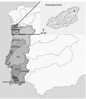
Statistical methodologies will be illustrated based on a rather extended data set relative to the River Ave basin in Northwest Portugal (Figure 1) and consist mainly of monthly measurements of physicochemical and microbiological variables in a network of water quality monitoring sites.
In the last thirty years, the River Ave hydrological basin has been subjected, with the exception of its upstream areas, to a growing rhythm of untreated effluent discharges from industrial activities, namely from the textile sector strongly implanted in this region. This whole situation is instrumental for the water quality deterioration, resulting in inappropriate water for several uses—human consumption, industrial use, recreational uses, fishing and irrigation—, thus posing a serious danger for public health (Oliveira et al., 2005).
Fig. 1. River Ave hydrological basin.
The River Ave hydrological basin has an approximate area of 1390 km2, from its source in Serra da Cabreira to its mouth in Vila do Conde; the main river length is 101 km and the average flow at the mouth is 40 m3/s. In the Northwest region of Portugal summer is dry and winter is mild with plenty of rain. So, the highest levels of precipitation take place between October and March: this represents 75 percent of the yearly precipitation. The main adjacent streams of River Ave are the River Este (flowing from the North) and the Rivers Selho and Vizela (from the South).
The River Ave differs from other Portuguese rivers not only because of its high pollution levels, but also because of the large spatial and temporal variability of pollutants concentration.
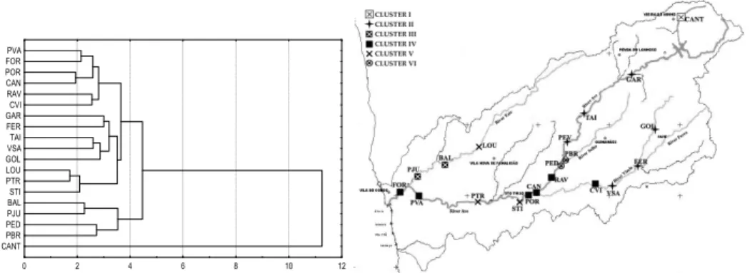
Since 1988, and as part of a national plan, the Central Administration—through the Northern Regional Directory for the Environment and Natural Resources—and the Institute of Water periodically (monthly) monitored the quality of surface water along the River Ave and its main adjacent streams by means of 20 monitoring sites: twelve of them are located in the River Ave’s mainstream: Cantelães (CANT), Garfe (GAR), Taipas (TAI), Pevidém (PEV), Pedome (PED), Riba d’Ave (RAV), Caniços (CAN), Portos (POR), Santo Tirso (STI), Ponte Trofa (PTR), Ponte Velha do Ave (PVA) and Formariz (FOR); Ponte Brandão (PBR) in the terminal segment of the adjacent stream River Selho; five in the adjacent stream River Vizela: Ferro (FER), Golães (GOL), Vizela Santo Adrião (VSA), Caldas de Vizela (CVI); and Louro (LOU), Balazar (BA) and Ponte Junqueira (PJU) in the adjacent stream River Este, (See Figure 2).
The data set comprises 11 quality variables: 10 physicochemical and a microbiological one (although there were more than 23 water quality variables available).
Fig. 2. Spatial distribution of the water quality monitoring sites of River Ave’s hydrological basin.
Physicochemical Variables Measurement Units
pH Sorensen scale
WT – Water Temperature °C(Celsius degrees)
COND – Conductivity μS cm/
TSS – Total Suspended Solids mg l/
DO – Dissolved Oxygen mgO2/l
OD – Oxygen Demand mgO2/l
COD – Chemical Oxygen Demand mgO2/l
BOD5 – 5-day Biological Oxygen Demand mgO2/l
NH4-N – Ammonical Nitrogen mgNH4/l
NO3-N – Nitrate-Nitrogen mgNO3/l
Microbiological Variables
FC – Faecal Coliforms nº/100ml
Table 1. Water quality variables and measurement units.
According to the National Department for Pollution Control, these are relevant variables for the evaluation of surface water quality of rivers subjected to industrial effluent discharges. Table 1 summarizes these water quality variables and their measurement units. An exploratory analysis of all 11 quality variables allowed a general diagnosis of surface water quality of this hydrological basin during the period under observation. The samples presented extreme values (too high or too low) which were not excluded because they can denote serious situations from an environmental point of view. These values were confirmed as far as possible. Taking into consideration that modelling and forecasting procedures will be performed, the data set is divided into two parts: one for modelling proposes (until September 2004) and another part for the forecast and assessment stage (until October 2006).
3. Multivariate statistical analysis
In this section, different methodologies will be applied in the field of Multivariate Statistics—Clusters Analysis (CA) and Principal Component Analysis (PCA)—with the aim of evaluating and interpreting the space-time variations of a large and complex amount of data on surface water quality of any given hydrological basin. These methodologies have allowed the identification of homogeneous regions (i.e., groups of monitoring sites with similar characteristics in terms of quality variables) and the obtention of classification patterns that enabled us to generate hypotheses about the revealed structure involving modifying phenomena and thus better understand the mechanisms responsible for the surface water quality of the River Ave’s basin.
The application of CA and PCA has achieved a meaningful classification of river water samples and has allowed the identification and assessment of spatial/temporal sources of variation affecting river water quality. In particular, cluster analysis (CA) allowed to reduce the large number of monitoring sites into a small number of homogeneous groups.
3.1 Cluster analysis
A first step consists of establishing a strategy to deal with a large data set collected in a group of water monitoring sites: for instance, twenty sites as in the present study case. CA is a group of multivariate techniques whose primary purpose is to assemble objects based on their characteristics (see Kaufman et al., 1990; Gordon, 1999, and Everitt et al., 2001). Hierarchical agglomerative clustering is the most common approach, providing intuitive similarity relationships between any given sample and the entire data set.
The strategy pursued in this paper follows a similar approach to Simeonov et al. (2003), Costa & Gonçalves (2011) and Gonçalves & Alpuim (2011), with the aim of geographically classifying homogenous groups of water quality monitoring sites based on water quality variables assessed by means of cluster analysis.
These approaches present different procedures in order to achieve the classification objectives. The first two papers consider clustering procedures that are implemented with a dissimilarity measure based on Euclidian distance and the last paper is performed with a dissimilarity measure based on Kullback information obtained in the state-space modelling process. It will be developed a discussion of its advantages and difficulties.
3.1.1 Cluster analysis of a global set of variables
In this study, hierarchical agglomerative CA was performed on the normalized data set (the 11 variables mentioned before). For the hierarchical agglomerative CA procedure purposes it will be considered the measure of dissimilarity proposed in Gonçalves & Alpuim (2011). The main problem is that for all locations and variables there are not observations for all months under study.
Therefore, let us consider xikt the value of the quality variable k, measured at location i, in time t. Let Pt be the set of all quality variables measured at the same time t, in sites i and j. The Euclidean distance between locations i and j at time t is given by the expression
CANT PBR PED PJU BAL STI PTR LOU GOL VSA TAI FER GAR CVI RAV CAN POR FOR PVA 0 2 4 6 8 10 12
Fig. 3. Dendrogram of the 11 quality variables without PEV and the spatial representation of River Ave’s clusters.
1 2 2 ( ) ( ) t ij ikt jkt k P dist t x x ∈ = −
. (1)This dissimilarity measure corresponds to the average of this distance over all months t, where there is at least one quality variable with measurements in the two sites, that is
1 2 2 1 ( ) # ij t ij ikt jkt ij t M k P d x x M ∈ ∈ = −
, with ,i j=1,...20 (2)where Mij is the set of all months with at least one variable measured in both sites i e j. The
monitoring sites Pevidém (PEV) and Ponte Trofa (PTR) are the only ones lacking simultaneous measurements for any given quality variable. In order to avoid this problem, in a first phase PEV was dropped from the construction process of the clusters since it was the location with the smallest number of observations. Later, PEV was included in the closest neighbouring cluster. In order to ascertain the dissimilarity between PEV and the cluster including PTR, the latter was not inputted into the calculations. The construction used three different hierarchical cluster methods—Ward’s, complete linkage and the unweighted pair-group average approach—because in this case they rendered well-defined clusters that were according to the reality of this particular river basin. As the results from the three methods are similar, the final result of the obtained groups was discussed according to the complete linkage method: in this method, the distance between the groups is defined as the distance between the most distant pair of objects, one from each group. According to the dendrogram analysis, we decided to form the clusters at a cut distance of d=3.4, thus obtaining six well-differenced clusters. The dendrogram of the monitoring sites obtained by means of the complete linkage method and the clusters geographical representation are shown in Figure 3. The resulting dendrogram has a cophenetic correlation coefficient of 0.85 (correlation coefficient between the original dissimilarity matrix and the “cophenetic matrix”), which validates the clustering procedure. Taking into consideration the quality variables averages within each cluster, they are classified into five
categories according to their pollution levels established by the National Department for Pollution Control (NDPC): "Without Pollution (WP)", "Moderately Polluted (MP)", "Polluted (P)", "Very Polluted (VP)" and "Extremely Polluted (EP)". Each cluster is classified based on the NDPC criteria which are determinated according to the worst value of a given variable observed in the cluster. The resulting classifications of the six clusters confirm the previous knowledge about effluent discharge according to the economic activities located along the basin. Also, the effect of these discharges on water quality varies according to natural and geographical/economical reasons.
Cluster I (consisting of just one monitoring site-CANT) may be characterized as Without Pollution and corresponds to the source of River Ave. Then there is a set of locations which can be defined as Moderately Polluted (Cluster II, composed by GAR, TAI, PEV, GOL, FER and VSA), including 6 sites in both adjacent streams Este and Vizela situated upstream the Rivers Ave and Vizela. These stations receive pollution mostly from domestic wastewater and from agricultural and manure discharges.
Cluster III, classified as Polluted 1 (P1), is composed by BAL and PJU located in River Este, where the quantity of nitrate-nitrogen has been relatively high (the River Este tends to present the largest problems in relation to this quality variable).
In Cluster IV, six of the monitoring sites (RAV, CAN, POR, PVA, FOR, and CVI) are situated in the River Ave and only one, CVI, at the most downstream site of River Vizela. In fact, the polluted area (Cluster IV) corresponds to the segment of the River Ave that goes from around the station RAV down to its mouth. This is a densely populated region, with high industrial productivity, and here the River Ave receives similarly polluted waters (Polluted 2 (P2)) from its adjacent rivers. In Cluster V, with three monitoring sites, LOU (in river Este, downstream of the Municipality of Braga), STI and PTR (located near the most polluted area of the Municipality of Ponte Trofa and Santo Tirso), there is a growing urban population and a high concentration of industrial activity. Cluster V was classified as Very Polluted. Finally, the most polluted cluster, Cluster VI (Extremely Polluted), consists of two monitoring sites, PBR and PED, located near the mouth of the Selho tributary and represents a highly polluted area. These monitoring sites receive pollution from domestic wastewater and industrial effluents located in city areas.
3.1.2 Cluster analysis for DO
As in Section 4, the analysis will focus on the modelling of Dissolved Oxygen (DO) concentration in water (measured in mg/l) because it is one of the most important variables in the evaluation of river water quality and because of its continuity in measurement at all selected water quality monitoring sites under analysis. This methodology intends to classify the water quality monitoring sites into spatial homogeneous groups based on the DO concentration, a variable considered relevant to characterize water quality. Furthermore, this type of analysis allows reducing the number of models in the modelling process. However, in this case the aim is to perform a clustering procedure for a univariate dimension, i.e., for a single water quality variable. Thus, the DO clustering procedure will be performed in an attempt to refine a methodology based on Kullback information measures that are obtained in the state space modelling process, as applied in Costa & Gonçalves (2011).
In order to identify homogeneous groups of water monitoring sites based on similarities in the temporal dynamics, we selected the modelling data sets by means of state space models and Kullback information measure, adapting here the methodology adopted in Bengtsson & Cavanaugh (2008). As the DO concentration showed much diversity regarding tendency and seasonality components in the River Ave and in its main adjacent rivers, we wanted to identify homogenous clusters of water monitoring sites considering the magnitude of DO concentration and then adopted a simple univariate state space model (SSM) for each location that considered DO in its true magnitude. By using a discrepancy measure suggested in Bengtsson & Cavanaugh (2008), we obtained a discrepancy matrix that allowed us to identify homogenous groups by applying clustering techniques.
In this modelling process are considered data series from 16 water monitoring sites (CANT, GAR, TAI, PBR, RAV, CAN, POR, STI, PTR, PVA, FOR, PJU, GOL, FER, VSA and CVI) between 1988 and 2006, because in the remaining four monitoring sites (PEV, PED, LOU, and BAL) the data is so scarce that it difficulted time modelling.
Briefly, it followed the main steps of the clustering proceeding. The discrepancy measure suggested in Bengtsson & Cavanaugh (2008) assumes that the variable Yi t, observed in location i at time t is modelled by a state space model as
, , , i t i t i t Y =X +e , (3) , ( , 1 ) , i t i i i t i i t X −μ φ= X − −μ +ε . (4)
where (3) is the measurement equation and (4) is the transition or state equation. As usually, errors ei t, and εi t, are uncorrelated white noises.
The unknown parameters { , , 2, 2}
i= μ φ σ σi i ε e
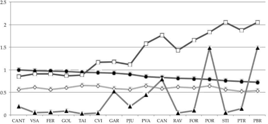
Θ in each location i are estimated by means of Gaussian maximum likelihood performed by EM algorithm (for more details, see subsection 4.1.3). Figure 4 reproduces parameters estimates for the 16 water monitoring sites.
The pseudo-distance between two monitoring sites i and j suggested by
Bengtsson &
Cavanaugh (2008), and
defined as a form of the J-divergence (Kullback, 1978), accounts for the different lengths of each series of data sets by averaging over time1 1
( , ; , ) ( , ; ) ( , ; )
X X X
i i j j i i i j j j j i
J Y Θ Y Θ =N d Y− Θ Θ +N d Y− Θ Θ . (5)
By employing output from the EM algorithm, including the maximum likelihood estimates, the sample J - divergence is given by X
2 2 ( ) ( ) ( ) ( ) ( ) ( ) 11 10 00 11 10 00 2 2 1 1 ˆ ˆ ( , ; , ) ( 2 ) ( 2 ) 1 ˆ ˆ 2 i 2 j j j j i i i X i i j j i i j j j i J Y Y S S S S S S Nσε φ φ Nσε φ φ = − + + − + − Θ Θ (6)
where smoothing quantities ( ) 11k S , ( )
10k S , ( )
00k
S and parameters estimates ˆΘ are computed k
based on the model ( ,Yk Θk). For more details, see Costa & Gonçalves (2011).
By using the parameters estimates of Figure 4 and the partial results of EM algorithm, the calculation of sample values X( ,ˆ ; ,ˆ )
i i j j
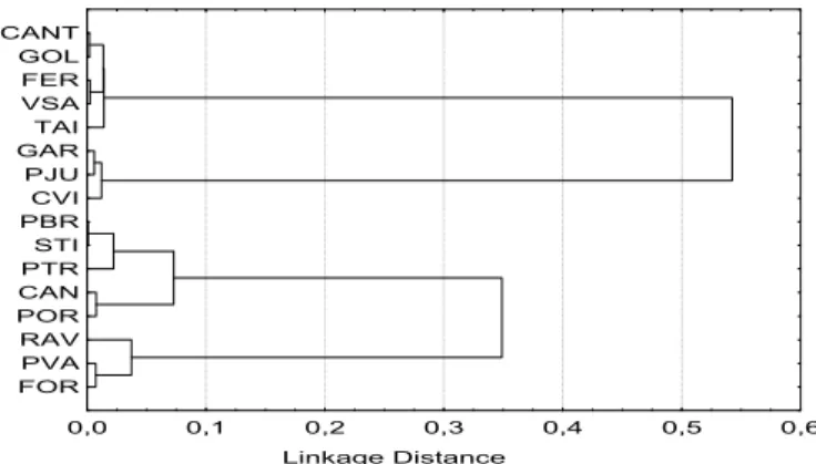
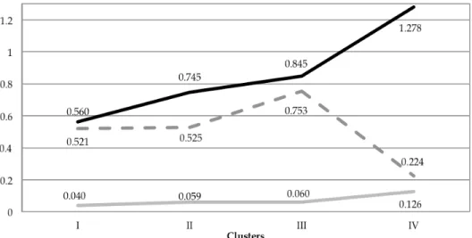
pseudo-distances. The discrepancy matrix was subjected to Ward’s, single linkage and complete linkage clustering procedures (Everitt et al., 2001). Because these three methods produced similar results, we only discussed the results obtaind through Ward’s method. As shown in the dendrogram in Figure 5, the identified clusters are comprised by sites: Cluster I (CANT, TAI, GOL, FER, VSA); Cluster II (GAR, PJU, CVI); Cluster III (RAV, PVA, FOR); and Cluster IV (PBR, CAN, POR, STI, PTR).
0 0.5 1 1.5 2 2.5
CANT VSA FER GOL TAI CVI GAR PJU PVA CAN RAV FOR POR STI PTR PBR
Fig. 4. Graphical representation of the parameters estimates to the 16 water monitoring sites ( - μˆ 10× −1, - φ, - ˆ
e
σ - ˆσε).
Considering the estimates of the processes mean obtained in the estimation procedure, it was clear that the clustering procedure performed a classification of the monitoring sites into a possible water quality scale in what concerns the annual mean DO concentration. In fact, the estimates of the processes mean in Cluster I monitoring sites presented the highest values obtained from DO concentration: the five monitoring sites of Cluster I presented the best water quality annual indicators, while the worst indicators are observed in Cluster IV monitoring sites. On the one hand, this methodology allowed classifying the water monitoring sites in four categories, considering the annual mean DO concentration: from best water quality (Cluster I) to worst water quality (Cluster IV). On the other hand, clustering procedure performs a discrimination of water monitoring sites based on state noise variance. Indeed, Cluster I corresponds to locations with the lowest state noise variances; Cluster II has state noise variances greater than Cluster I, and so on. Since the discrepancy measure tends to compare state densities ( | )f Xi Θi and ( |f X Θ , j j)
it is natural that clustering procedure depicts some patterns on the parameters of these distributions.
It is interesting to note that Cluster IV has water monitoring sites located downstream the confluences of Rivers Selho and Vizela, i.e., where the River Ave receives highly polluted waters from these adjacent streams. The water monitoring sites located in this middle stretch of the River Ave are much more polluted, probably because they are close to densely populated areas with high industrial production units.
Linkage Distance FOR PVA RAV POR CAN PTR STI PBR CVI PJU GAR TAI VSA FER GOL CANT 0,0 0,1 0,2 0,3 0,4 0,5 0,6
Fig. 5. Dendrogram showing the clustering of monitoring sites according to DO characteristics based on Ward’s method.
3.2 Principal Component Analysis
The Principal Component Analysis (PCA) is designed to transform the original variables into new, uncorrelated variables called the principal components (PCs), which are linear combinations of the original variables (see Barnett, 1981, and Johnson et al., 1992). PCA allows us to explain and evaluate the correlation structure between observed variables in water quality sampling stations and to identify relevant factors. The PCA technique is separately applied to the homogeneous groups of water monitoring sites (six clusters), as obtained in the first clustering procedure, by taking into account all 11 water quality variables.
The Kaiser-Meyer-Olkin (KMO) statistics and Bartlett’s test were performed in order to examine the data suitability for PCA. High values (close to 1) generally indicate that the principal component analysis may be useful, as is the case in this study (KMO=0.85). Also, the significance levels for Bartlett’s test under 0.05 in this study indicate that there are significant relationships among variables.
Spearman rank-order correlations were used to study the correlation structure between variables in order to account for non-normal distribution of water quality variables.
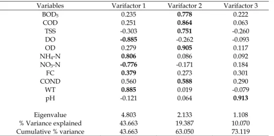
PCA was separately performed on the raw data sets (11 variables) for the six different regions (clusters) WP, MP, P1, P2, VP and EP, as delineated by CA techniques, in order to compare the compositional pattern among the analysed water monitoring sites and to identify the factors influencing each one. To further reduce the contribution of variables with minor significance, the PCs were subjected to varimax rotation (raw) generating varifactors (VFs). The PCA of the six data sets yielded four PCs for the WP and MP monitoring sites, three PCs for the P1, P2, VP and EP monitoring sites with eigenvalues >1, explaining 69.86, 63.52, 69.91, 69.31, 65.66 and 73.12 of the total variance in the respective water quality data sets. An eigenvalue gives a measure of the factor significance: the factors with the highest eigenvalues are the most significant. Eigenvalues of 1.0 or greater are considered significant. Corresponding VFs, variable loadings and explaining variance are obtained for six clusters. In this chapter we will only present the results for Cluster VI (EP), in Table 2, and then their respective interpretation.
Variables Varifactor 1 Varifactor 2 Varifactor 3 BOD5 0.235 0.778 0.222 COD 0.251 0.864 0.063 TSS -0.303 0.751 -0.260 DO -0.885 -0.262 -0.093 OD 0.279 0.905 0.117 NH4-N 0.806 0.086 0.092 NO3-N -0.776 -0.171 0.184 FC 0.379 0.273 0.301 COND 0.560 0.588 0.290 WT 0.885 0.019 -0.079 pH -0.121 0.064 0.913 Eigenvalue 4.803 2.133 1.108 % Variance explained 43.663 19.387 10.070 Cumulative % variance 43.663 63.050 73.119
Table 2. Loadings of experimental variables (11) on the first three rotated PCs for EP sites data set (Bold values indicate the most important loadings).
Concerning the data set pertaining to EP sites, and based on the group of information resulting from the water quality analysis of the monitoring sites PBR (in River Selho) and PED (in River Ave), among the three varifactors kept in the application of ACP, Varifactor 1 explains 43.66 percent of the total variance, has strong negative loadings on the variables DO and nitrate-nitrogen and also strong positive loadings on ammonical nitrogen and temperature variables. This varifactor contains the variables most related to pollution of anthropogenic origin.
The same happens with Varifactor 2, which explains 19.38 percent of the total variance and presents strong positive loadings on BOD5, COD, TSS, OD and COND. This organic factor can be interpreted as representing influences from point sources such as discharges from domestic wastewater and industrial effluents, but it cannot be interpreted only in terms of organic pollution, because it is also participated by the conductivity (mineral composition of the water).
Varifactor 3 explains 10.07 percent of the total variance, with strong positive loadings on pH, and presents the influence of this variable in the chemical processes in extremely polluted waters, from the nitrification processes of the nitrogen to the deposition of heavy metals. It is known that this basin’s water should present low pH values (a natural characteristic of its own geomorphology). It is known that the River Selho is heavily polluted by the urban and industrial sewage of Guimarães and Pevidém, and so this varifactor reflects these modifier phenomena responsible for this serious environmental situation.
The obtained latent multifactors, with hydrochemical meaning, indicate that the responsible variables for the variation of the basin’s water quality are mainly related with effluent discharges of anthropogenic origin (agricultural domestic and industrial origin) along the River Ave and its tributary streams. Only in areas Without Pollution or Moderately Polluted
do latent factors represent the variability inherent to the natural climatic seasonality and the variability associated to the basin’s geomorphological characteristics, both of which naturally influence the hydrochemistry of the rivers’ surface water.
Although the principal component analysis did not result in a significant data reduction— by explaining the correlation among a set of variables in terms of a small number of principal components without losing much information—, nonetheless it helped to extract and identify the factors/sources responsible for variations in the rivers’ water quality at six different sampling sites, and it also allowed to assess associations among variables, since they indicate the participation of individual physicochemical and microbiological variables in several influence factors. Varifactors obtained from component analysis indicate that the quality variables responsible for water quality variations are mainly related to discharge and temperature (natural origin), nutrients and organic pollution in relatively less polluted areas, pollution by organic matter and nutrients from anthropogenic sources (mainly as discharges of industrial and municipal wastewater), and manure affecting the quality and hydrochemistry of river water in highly polluted areas in the basin. For instance, in the less polluted group it is identified the most significant varifactor with positive weights in faecal coliforms (FC), water temperature (WT), and high negative weight in DO concentration. This means that high water temperatures associated with water contamination by organic matter cause an increase in the lack of DO in water. By contrast, in a group classified as “Very Polluted”, the first varifactor (with 45.51 percent of the total variance) incorporates a significant set of organic-type variables, conductivity (COND) and pH variables. Besides representing an organic factor, it indicates anaerobic fermentation, hydrolysis of materials and the presence of mineral products (inorganic). This shows the strong influence of anthropogenic pollution in the much polluted clusters.
4. Statistical modelling of DO concentration
In this section, a temporal statistical analysis is exposed to illustrate the potential of some statistical approaches which, when combined, can be useful in understanding the evolution of water quality within a watershed. The starting point is based on the study case presented in Costa & Gonçalves (2011) that is developed and discussed here. Although there are more water quality variables available, DO concentration was selected due to its continuity in measurement at all selected water quality monitoring sites and to its importance in the evaluation of river water quality. The DO concentration analysis measures the amount of gaseous oxygen (O2) dissolved in an aqueous solution. Oxygen gets into water by diffusion from the surrounding air by aeration and as a waste product from photosynthesis.
The DO in water is one of the most important quality variables to assess the degree of pollution existent in the surface waters of a river’s hydrological basin. Low values indicate bad water quality. Oxygen levels also can be reduced through over-fertilization of water plants by run-off from farm fields containing phosphates and nitrates. DO concentration can be affected by organic pollution, which is the most common type of pollution in the River Ave’s basin, and consequently, a frequent problem is a deficit of DO. This could be aggravated by the existence of a sequence of small dams in the River Ave and in its main adjacent rivers, which limit the oxygen’s transfer by aeration. DO concentration is also affected by temperature: indeed, if water is too warm and there are too many bacteria or aquatic animal in the area, they may overpopulate, using DO in great amounts.
The evolution of DO concentration in the River Ave’s basin is evaluated considering the clustering results presented in subsection 3.1.2. Thus, the modelling procedure will be performed for each cluster.
4.1 Prediction models
In order to satisfy prediction purposes, prediction models as linear regression models and state-space models are considered for each cluster. These approaches allow discussing the mode of incorporating seasonality and trend components in prediction models because state-space models integrate a dynamic structure that incorporates time dependence sometimes presented in environmental data.
Usually, linear models are preferred in respect to more complex models for being a primary tool in the context of environmental problems. Linear models are simple, have good statistical properties and are very robust statistical methods, which makes them a very attractive framework to describe the quality variables under study. However, the standard linear regression model does not include a possible time dependence of data. If errors of the linear models are correlated, the standard deviations of the coefficients given by linear model are not corrected, which may lead to a wrong decision given by the t-test. It is possible to overcome these difficulties considering that errors follow an AR(p) Gaussian stationary process. For more details, see Alpuim & El-Shaarawi (2008). Alternatively, in this work it is considered a linear state-space model whose formulation as presented can be interpreted as a calibration model of seasonal coefficients. As it will be shown, this formulation will allow making some useful interpretations.
4.1.1 Linear regression approach
Standard linear regression models are fitted to DO concentration data. In this case study, the authors consider that the observations at different locations in the cluster are treated as independent observations referenced in time, because there is no measure of space continuity.
Within each cluster it is considered a variable observation ( ) ,i
j t
Y , where i represents the cluster, i=1,2,3,4, j represents the monitoring site running along all sites in the cluster i,
1,2,..., i
j= k and 1,2,.., ( )i j
t= n stands for the month. In order to contemplate both trend and seasonal components, the model in cluster i includes two additive components besides the error, that is,
( ) ( ) ( ) ( ) ,i ti ti i,
j t j t
Y =T +S +e . (7)
After a graphical inspection, the trend is considered a simple linear function of time ( )i ( )i ( )i
t
T =α +β t. The seasonal component ( )i t
S is a periodic function taking 12 different values ( )i
s
λ with s=1,...,12 associated with each month of the year, that is, ( )
1, if date corresponds to month 1, if date corresponds to month 12 0, otherwise i t t s S t = − . (8)
Cluster I Cluster II Cluster III Cluster IV Intercept 9.197 9.867 8.634 7.711 Trend 0.004 -0.009 -0.003 - January 0.960 1.382 2.045 2.540 February 1.117 1.410 2.122 2.457 March 0.602 0.577 0.983 1.323 April - 0.784 0.708 1.027 May - - - - June -0.440 -1.093 -1.025 -1.352 July -1.160 -1.557 -3.143 -3.391 August -1.426 -2.037 -1.755 -1.501 September -0.980 -0.912 -2.441 -3.240 October -0.520 -0.546 -0.780 -1.143 November 0.720 0.711 1.183 1.118 December 1.125 1.281 2.103 2.161 2( ) ˆ i σ 0.854 1.019 1.198 1.766 R2 0.50 0.58 0.69 0.57
Table 3. Results for the linear models adjustment to the four clusters.
Note that the seasonal component is described with 12 dummy variables. In order for these parameters to be estimable, when the model has a constant term it is considered the restriction 12 ( ) 1 0 i s s= λ =
with ( ) 11 ( ) 12i s 1 siλ = −
= λ . The choice of the twelfth month to be written as a linear combination of others is arbitrary. The model includes a stochastic term, e , ( )j ti, which is taken as a sequence of uncorrelated zero mean random variables, with constant variance σ2( )i .In order to ensure the optimality properties of Ordinary Least Squares (OLS) method as the power of the t and F tests performed, a check of residuals shows that there were no significant violations of the normality. In order to obtain the final models, one for each cluster, it is used a backwards elimination procedure to select the significant variables. Thus, at each step, the regressor with the largest p-value for its t-statistics was removed, until all regressors were significant at level 0.05.
Table 3 presents the final results of the linear models’ fitting to the four clusters. Briefly, as expected, the models adjustments show a seasonal pattern with lower values of DO concentration in the warmer months as compared to fall and winter months. Three clusters present weak trends: Cluster I shows a positive trend and Cluster II and III show a weak decreasing trend. The most polluted cluster does not present a significant trend, i.e., it has a stable behaviour, which may be justified if taken the highest error variance estimate into consideration.
4.1.2 State-space approach
State-space models are very versatile and can assume several state-space representations, namely by including linear models. For instance, if regression parameters β of the usual
linear model Y βX= may vary over time, i.e., βt, the model may be treated as a dynamic
model, thus admitting a state-space representation.
In order to identify possible changes over time, namely in trends, it is formulated a linear state-space model that takes into account only a seasonal component, since trends in linear models—even when trend is statistically significant—is very weak.
Thus, for cluster i it is considered the state-space model ( )i ( ) ( )i i ( )i t = t βt + t Y S e (9) ( ) ( ) ( ) ( ) 1 1 ( i 1) i i i t t t β = +φ β− − + ε . (10)
The observation equation (9) relates the ki×1 vector of observed DO concentration in the ki
monitoring sites of cluster i at month t, Yt( )i , with the seasonal coefficient (mean value) of
month t of cluster i, s , by means of a product of a stochastic calibration factor ( )ti β( )ti by
( ) ( ) ( )i
i i
t = n st
S 1 and adding to a zero mean vector error e( )ti . Note that 1( )ni represents a single
matrix column ni×1 with all elements equal to the unity.
It is assumed that the state, or in this case the calibration factor β( )ti , follows a stationary
autoregressive process of order 1, AR(1), i.e., |φ( )i| 1< , with unitary mean, expressed by (10).
Both errors e( )ti and εt( )i are uncorrelated white noises with constant variances
( ) ( ) 2,( ) [ i i] i i
t t e k
Ee e′ =σ I and E[εt2,( )i]=σε2,( )i .
The state-space model (9) – (10) associated to the Kalman filter allows predicting calibration factor values at each month taking into account observed data up to that month (filtered predictions) and, if useful, one-step forecasts. An additional advantage of this approach consists of the filtered prediction of the calibration factor β( )ti as a measure of the
discrepancy between the observed value of the quality variable in a given month and the excepted value (the seasonality mean value) for this month.
For instance, if a calibration factor is predicted at 1.05 it means that this month’s DO concentration value exceeded the seasonal coefficient of 5 percent. Thus, calibration factor predictions allow analysing the temporal dynamic of DO concentration by taking into account the expected structure translated by seasonal coefficients.
For each cluster it is necessary to estimate a set of parameters Θ =( )i {φ σ( )i, e2,( )i,σε2,( )i}. If the errors are normally distributed, the conditional log-likelihood of the random
( ) ( ) ( ) 1 2 (Yi,Yi,...,Yni) can be written as
( )
( )
( ) ( ) ( ) ( ) ( ) ( ) 1,( ) ( ) 1 2 1 1 1 1log ( ; , ,..., ) log 2 log
2 2 2 i i i n n i i i i i i i i i t t t t n t t n L π − = = ′ = − −
−
Θ Y Y Y Ω η Ω η (11) where ( ) ( ) ( ) | 1 i i i t t pt t− t′ Ω =S S and ( ) ( ) ( ) | 1 ˆ i i i t t t tη =Y −Y − is the innovation (note that pt t| 1− and Yˆt t( )| 1i−
are obtained by Kalman filter algorithm: see the Annex).
Thus, it is possible to obtain the maximum likelihood estimates by maximizing the conditional log-likelihood in order to obtain the unknown parameters Θ( )i , for each cluster
1,2,3,4
i= , by using numerical algorithms, namely the EM or the Newton-Raphson algorithms. Figure 6 reproduces estimates obtained in Costa & Gonçalves (2011). It is quite clear that the adopted approach reveals the differences between clusters in the context of DO concentration. As expected, the standard deviations estimated from the calibration factors are lower than the standard deviations resulting from the observation of the equations errors. Indeed, the state-space model separates two sources of variability reflected in two errors: observation and state equations. Thus, it is reasonable that calibration factors have less variability while the observation errors incorporate measurement errors and, most importantly, sporadic and unpredictable events as illegal pollutants discharges, among others. However, Cluster IV stands out from others because it presents the largest variability in error equation as much as in state equation error. So, Cluster IV presents the worst monthly averages of DO concentration but it also shows the highest variability.
Fig. 6. Graphical representation of the four clusters estimated values via Gaussian maximum likelihood ( - ˆφ, - ˆσε, - ˆσe).
4.1.3 Model’s adjustment discussion
As mentioned before, the modelling process focuses on a subset of available data. The remaining data (from October 2004 to October 2006) was used to assess forecast performance of models. Costa & Gonçalves (2011) shows that the state-space approach provides the least Root of the Mean Square Errors of forecasts (RMSE). Indeed, the RMSE obtained in state-space models was RMSE=0.846, while in the linear regression models the result was RMSE=0.961. Thus, the state-space approach improved the forecast accuracy in the sense of the mean square error of forecasts. Besides providing better forecasts of DO concentration, the state-space approach allows analysing temporal evolution in a dynamic way by observing calibration factor predictions. Other potentialities of the state-space models will be explored in the next section.
4.2 Online water quality monitoring by using Kalman filter predictions
The forecast accuracy is not always the most important characteristic of a model. Indeed, in water quality monitoring it is useful to analyse temporal evolution in order to identify possible factors or changes. This analysis can be performed in two ways:
- trends analysis by looking into the historical data; - dynamic or online procedure.
The first approach can be achieved largely through linear regression models by analysing trends parameters and it allows diagnosing any global tendency (linear or other, as exponential, polynomial, etc.) that can be statistically significant.
Thus, the next discussion focuses on the dynamic monitoring procedure based on the state-space approach (associated to the Kalman filter algorithm). Indeed, the state-state-space approach adds a dynamic component to the usual linear models that can be useful in the water quality monitoring procedure. Considering that the DO concentration at each month can be regarded as an updated value of the expected value for a given month st (seasonal
coefficient), that update is done by a multiplicative factor βt by the observation equation t = t tβ + t
Y S e , (12)
and so the online prediction of βt for each month t by Kalman filter algorithm indicates
how much any given monthly DO concentration diverges from the its monthly average. In order to achieve this, it is necessary to compute filtered values of βt (in this case for all
clusters) for all months.
Given the probability distribution of predictor βˆt t|,
(
)
| |
ˆ ~t t N t,pt t
β β , (13)
the 95% point-wise prediction intervals are computed by the boundaries
| |
ˆt t 1.96 pt t
β ± , (14)
where βˆt t| is the filtered value of βt when Yt is observed and p is the estimated MSE of t t| |
ˆt t
β . If the DO concentration measurement shows no statistical change in comparison to the monthly mean, then, according to the statistical inference theory, the unity must be in the point-wise prediction interval corresponding to that month, that is,
| | | |
ˆ ˆ
1∈βt t−1.96 pt t,βt t+1.96 pt t
(15)
considering a significant level of 5%.
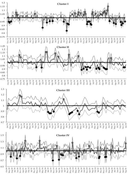
Figure 7 represents the 95% point-wise predictions intervals for the four clusters. This procedure allows revealing the monthly measurements that are statistically different from the global seasonal component, because the value is higher or lower than the expected.
Fig. 7. Graphical representation of the 95% point-wise predictions intervals for the four clusters. Symbols and indicate that DO concentration is statistically higher or lower than the correspondent seasonal coefficient, respectively.
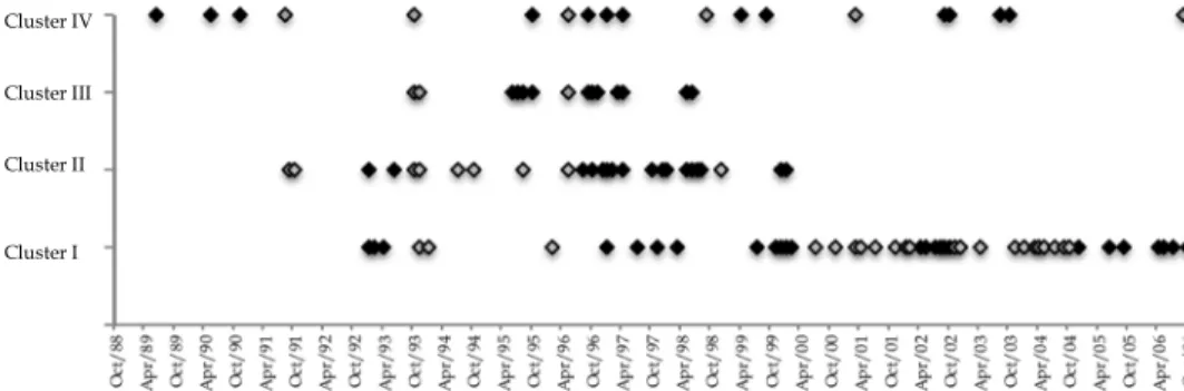
Cluster I results show that there were two periods of high water quality besides the expectation, namely from July 2000 to February 2002, and from November 2002 to October 2004. Since December 2004 some measurements indicate water quality deterioration in comparison to the expected results. For Cluster II, during a significant number of months from August 1996 to August 1998 the DO concentration measurements show lower values than the expected, while up to this time there were some sporadic months with a significant statistical difference in relation to seasonal coefficient. The graphical representation in the case of Cluster III presents two short time periods with lower relative values of DO concentration, from June 1995 to October 1995, and from September 1996 to April 1997. Cluster IV (the most polluted one) does not present evident periods of water quality improvement or deterioration and sporadically shows statistical unexpected values. Table 4 summarizes the percentage of months with DO concentration values that are statistically different from the expected. Clusters I, II and III show higher percentages than Cluster IV. This result is consistent with the linear regression results, in which these clusters present significant linear trends. In order to analyse the four clusters global behaviour, Figure 8 shows a simultaneous graphical representation of the months that were identified in the previous procedure. This representation shows that there are periods with a consistent behaviour in the generality of the clusters: for instance, from October 1993 to January 1994 were identified higher values of DO concentration, or from September 1996 to June 1998, where the DO concentration was lower than the expected in the whole area of the river basin. Cluster - + Total I 15% 13% 28% II 15% 8% 23% III 13% 4% 16% IV 6% 3% 9%
Table 4. Percentages of months during which DO concentration values are statistically different from the seasonal coefficients per cluster. Symbols “+” and “-”indicate whether the difference is by excess or defect, respectively.
Cluster II Cluster IV Cluster III
Cluster I
Fig. 8. Graphical representation of the most significant values for the four clusters over the same time axis. Symbols and indicate that DO concentration is statistically higher or lower than the correspondent seasonal coefficient, respectively.
5. Conclusion
The several statistics techniques applied in this work allow an integrate analysis of some environmental data dimensions, particularly of water quality data. The combination of multivariate statistical methodologies (as, for instance, CA and ACP procedures) with the temporal dimensions (as in linear and state-space approaches) has shown to be very useful in order to obtain global and more accurate results. For instance, hierarchical cluster analysis grouped 20 monitoring sites into six clusters of similar water quality characteristics and, based on the obtained information; it is possible to design a future, optimal spatial sampling strategy which could reduce the number of sampling monitoring sites and associated costs. The results of CA confirm the expected behaviour of the temporal/spatial dynamics of pollutants concentration (along the river and its main streams) and agree with those produced by the performed classification, thus allowing to reduce the large number of monitoring sites into a small number of homogeneous groups and yields an important data reduction.
An important conclusion from the CA procedure is the possibility of obtaining groups that can be classified according to their pollution level, as established from a set of criteria, and taking into account spatial and time dimensions.
The ACP analysis indicates that clusters have distinct factors/sources responsible for variations in River Ave’s water quality and it helps to identify environmental, social and industrial aspects which influence water quality variations. The varifactor analysis shows very clearly that the industrial activity location has an impact on water quality.
Linear models and state-space models showed to be complementary in accordance to the proposed objectives. Linear models are useful when it is needed to identify global trends. State-space models have proven to be more accurate when the main objective is to obtain an accurate forecast of DO concentration. In addition, the state-space approach allows doing an online monitoring procedure to detect DO concentration values that are statistically unexpected. On the other hand, the state-space formulation presented in this work performs the measurement in percentage variation from the observed value of the seasonal coefficient. The statistical modelling procedure was applied to a set of water monitoring sites grouped in homogeneous clusters. However, the modelling methodology can be applied to a single time series of any given quantitative water quality variable in a single location. This combination of statistical methodologies can be applied to other environmental issues, because statistical techniques are very versatile.
6. Annex
Briefly, the Kalman filter is an iterative algorithm that produces an estimator of the state vector
t
X at each time t, which is given by the orthogonal projection of the state vector onto the observed variables up to that time. Considering the general formulation of a state-space model
t= t t+ t
Y H X e . (16)
1
t= t− + t
X ΦX ε . (17)
Let Xˆt t| 1− represent the estimator of Xt based on the information up to time t−1, that is, based on Y1, Y2, …, Yt−1, and let Pt t| 1− be its mean squared error (MSE) matrix. As the orthogonal projection is a linear estimator, the predictor for the next variable, Yt, is given by
| 1 | 1
ˆ ˆ
t t− = t t t−
Y H X . (18)
When, for time t, Yt is available, the prediction error or innovation, ηt=Yt−Yˆt t| 1− , is used
to update the estimate of Xt through the equation
| | 1
ˆ ˆ
t t= t t− + t tη
X X K , (19)
where Kt is called the Kalman gain matrix and is given by
(
)
1 | 1 | 1 t t t t t t t t − − ′ − ′ = + e K P H H P H Σ .
Furthermore, the MSE of the updated estimator X verifies the relationship ˆt t|
| | 1 | 1
t t= t t− − t t t t−
P P K H P . In turn, for time t, the forecast for the state vector Xt+1 is given by the equation Xˆt+1|t=ΦXˆt t| and its MSE matrix is Pt+1|t=ΦP Φt t| ′+ Σε.
This recursive process needs initial values for the state vector, X , and for its MSE, 1|0 P , 1|0 that will be later seen in more detail. As usual, the orthogonal projection corresponds to the best linear unbiased predictor. When the disturbances et and εt are normally distributed,
the state vector and the observed variables are also normal. Therefore, in this case the orthogonal projection is also the conditional mean value and the Kalman filter is optimal.
7. Acknowledgments
This research was partially financed by FEDER Funds through "Programa Operacional Factores de Competitividade – COMPETE" and by Portuguese Funds through FCT - "Fundação para a Ciência e a Tecnologia", within the Project Est-C/MAT/UI0013/2011. A. Manuela Gonçalves was partially financed by FEDER Funds through "Programa Operacional Factores de Competitividade – COMPETE" and by Portuguese Funds through FCT - "Fundação para a Ciência e a Tecnologia", within the Project Est-C/MAT/UI0013/2011. Marco Costa was partially supported by Fundação para a Ciência e a Tecnologia, PEst OE/MAT/UI0209/2011.
8. References
Alpuim, T. & El-Shaarawi, A. (2008). On the efficiency of regression analysis with AR(p) errors. Journal of Applied Statistics, Vol.35, No.7, pp. 717-737
Ato, A., Samuel, O., Óscar, Y. & Moi, P. (2010). Mining and heavy metal pollution: assessment of aquatic environments in Tarkwa (Ghana) using multivariate statistical analysis. Journal of Environmental Statistics, Vol.1, No.4, 1-13
Barnett, V. (1981). Interpreting Multivariate Data, John Wiley & Sons, Sheffield
Bengtsson, T. & Cavanaugh, J.E. (2008). State-space discrimination and clustering of atmospheric time series data based on Kullback information measures. Environmetrics, Vol.19, No.2, pp. 103-121
Costa, M. & Gonçalves, A.M. (2011). Clustering and forecasting of dissolved oxygen concentration on a river basin. Stochastic Environmental Research and Risk Assessment, Vol.25, No.2, pp. 151-163
Elhatip, H., Hinis, M. & Gülbahar, N. (2008). Evaluation of the water quality at Tahtali dam watershed in Izmir-Turkey by means of statistical methodology. Stochastic Environmental Research and Risk Assessment, Vol.22, No.3, pp. 391-400
EU (2000). Directiva 2000/60/CE do Parlamento Europeu e do Conselho, de 23 de Outubro de 2000 (DQA, 2000), Estabelece um Quadro de Acção Comunitária no Domínio da Política da Água. Jornal Oficial das Comunidades Europeias, L327:1-72
Everitt, B., Dunn, G. & Leese, M. (2001). Cluster Analysis, 4th Edition, Arnold, London Gonçalves, A. & Alpuim, T. (2011). Water Quality Monitoring using Cluster Analysis and
Linear Models. Environmetrics, DOI:10.1002/env.1112 Gordon, A. (1999). Classification, Chapman and Hall/CRC, London
Helena, B., Pardo, R., Vega, M., Barrado, E., Fernandez, J. & Fernandez, L. (2000). Temporal evolution of groundwater composition in an alluvial aquifer (Pisuerga river, Spain) by principal component analysis. Water Research, Vol.34, No.3, pp. 807-816
INAG, I.P. (2008a). Tipologia de Rios em Portugal Continental no âmbito da implementação da Directiva Quadro da Água. I-Caracterização Abiótica, Ministério do Ambiente, do Ordenamento do Território e do Desenvolvimento Regional, Instituto da Água, I.P. INAG, I.P. (2008b). Manual para a avaliação biológica da qualidade da água em sistemas
fluviais segundo a Directiva Quadro da Água-Protocolo de amostragem e análise para os macroinvertebrados bentónicos. Ministério do Ambiente, do Ordenamento do Território e do Desenvolvimento Regional, Instituto da Água, I.P.
Johnson, R. & Wichern, D. (1992). Applied Multivariate Statistical Analysis, 3rd Edition, Prentice-Hall
Kaufman, L. & Rousseeuw, P. (1990). Finding Groups in Data: An Introduction to Cluster Analysis, John Wiley & Sons, New York
Lischeid, J. (2009). Non-linear visualization and analysis of large water quality data sets: a model-free basis for efficient monitoring and risk assessment. Stochastic Environmental Research and Risk Assessment, Vol.23, No.7, pp. 977-990
Liu, C.W., Lin, K.H. & Kuo, Y.M. (2003). Application of factor analysis in the assessment of ground-water quality in a blackfoot disease area in Taiwan. The Science of the Total Environment, Vol.313, No.1-3, pp.77-89
Machado, A., Silva, M. & Valentim, H. (2010). Contribute for the evaluation of water bodies status in Northern Region. Revista Recursos Hídricos, Vol.31, No.1, pp. 57-63
Oliveira, R.E.S., Lima, M.M.C.L. & Vieira, J.M.P., (2005). An Indicator System for Surface Water Quality in River Basins. In The Fourth Inter-Celtic Colloquium on Hydrology and Management of Water Resources, Universidade do Minho, Guimarães, Portugal Shrestha, S. & Kazama, F. (2007). Assessment of surface water quality using multivariate
statistical techniques: A case study of the Fuji river basin, Japan. Environmental Modelling & Software, Vol.22, No. 4, 464-475
Simeonov, V., Stratis, J., Samara, C., Zachariadis, G., Voutsa, D., Anthemidis, A., Sofoniou, M. & Kouimtzis, Th. (2003). Assessment of the surface water quality in Northern Greece. Water Research, Vol.37, No.17, 4119-4124
Varol, M. & Sen, B. (2009). Assessment of surface water quality using multivariate statistical techniques: a case study of Behrimaz Stream, Turkey. Environmental Monitoring and Assessment, Vol.159, No.1-4, pp. 543-553
Vega, M., Pardo, R., Barrado, E. & Debán, L. (1998). Assessment of seasonal and polluting effects on the quality of river water by exploratory data analysis. Water Research, Vol.32, No.12, 3581-3592
Vieira, J.M.P. (2003). Water management in national water plan challenges. Revista Engenharia Civil, Vol.16, pp.5-12
Wurderlin, D.A., Diaz, M.P., Ame, M.V., Pesce, S.F., Hued, A.C. & Bistoni, M.A. (2001). Pattern recognition techniques for the evaluation of spatial and temporal variations in water quality. A case study: Suquia river basin (Cordoba-Argentina). Water Research, Vol.35, No.12, pp. 2881-2894