Probing the CP nature of the Higgs coupling in $t{\bar t}h$ events at the LHC

(1)

Probing the CP nature of the Higgs coupling in t¯

th events at the LHC

S. Amor dos Santos1_{, M.C.N. Fiolhais}1,2_{, R. Frederix}3_{, R. Gonçalo}4_{, E. Gouveia}5_{, R.}

Martins5, A. Onofre5, C.M. Pease5, H. Peixoto6, A. Reigoto5, R. Santos5,7,8, J. Silva6

1 _{LIP, Departamento de Física, Universidade de Coimbra, 3004-516 Coimbra, Portugal}

2 _{Department of Science, Borough of Manhattan Community College, City University of New York,}

199 Chambers St, New York, NY 10007, USA

3 _{Physik Department T31, Technische Universität München, James-Franck-Str. 1, D-85748 Garching, Germany}

4 _{LIP, Av.} _{Elias Garcia, 14-1, 1000-149 Lisboa, Portugal}

5 _{LIP, Departamento de Física, Universidade do Minho, 4710-057 Braga, Portugal}

6 _{Centro de Física, Universidade do Minho, Campus de Gualtar, 4710-057 Braga, Portugal}

7 _{Instituto Superior de Engenharia de Lisboa - ISEL, 1959-007 Lisboa, Portugal}

8 _{Centro de Física Teórica e Computacional, Faculdade de Ciências,}

Universidade de Lisboa, Campo Grande, Edifício C8 1749-016 Lisboa, Portugal

Abstract

The determination of the CP nature of the Higgs coupling to top quarks is addressed in this paper, using t¯th events produced

in√s = 13 TeV proton-proton collisions at the LHC. Dileptonic final states are employed, with two oppositely charged leptons

and four jets, corresponding to the decays t → bW+ → b`+

ν`, ¯t → ¯bW− → ¯b`−¯ν` and h → b¯b. Pure scalar (h = H),

pure pseudo-scalar (h = A) and CP-violating Higgs boson signal events, generated with MadGraph5_aMC@NLO, are fully reconstructed through a kinematic fit. We furthermore generate samples that have both a CP-even and a CP-odd component

in the t¯th coupling in order to probe the ratio of the two components. New angular distributions of the decay products, as

well as CP angular asymmetries, are explored in order to separate the scalar from the pseudo-scalar components of the Higgs

boson and reduce the contribution from the dominant irreducible background, t¯tb¯b. Significant differences between the angular

distributions and asymmetries are observed, even after the full kinematic fit reconstruction of the events, allowing to define the best observables for a global fit of the Higgs couplings parameters.

INTRODUCTION

On July 2012, the discovery of a Higgs boson, predicted by the electroweak symmetry breaking mechanism [1] of the Standard Model (SM) of particle physics, with a mass close to 125 GeV, was announced by both ATLAS [2] and CMS [3] collaborations. Since then, studying the Higgs boson properties has motivated many physics analyses at the LHC. So far, the measured properties of the Higgs boson have shown remarkable consistency with those pre-dicted by the SM [4]. Nevertheless, it is by now clear that the SM cannot explain all the observed physical phenom-ena. One of the best known examples is that it fails to explain the matter anti-matter asymmetry of the Uni-verse, for which new sources of CP-violation beyond the SM (BSM) are required. One possibility would be to in-troduce CP violation in the Higgs sector. This is allowed in BSM models, such as supersymmetry and 2-Higgs dou-blets models (2HDM), where the Higgs boson(s) have no definite CP quantum number resulting in a Yukawa cou-pling with two components, one CP-even and one CP-odd (see for instance [5]).

Analyses focusing on the Higgs boson decays to pho-tons, ZZ and W W , as well as on the V H (V = W, Z) as-sociated production have been conducted to measure its spin and parity quantum numbers [6–8]. All the results are consistent with a SM-like spin 0, parity even boson, while the pure pseudoscalar scenario has been excluded at a 99.98% confidence level (CL). However, the possibility of a CP admixture manifestation in the Yukawa couplings remains to be probed directly. So far only CP-odd

com-ponents of the Higgs couplings to the weak gauge bosons were shown to be very small. Within all fermions, the top quark is expected to have the largest Yukawa coupling. Currently, this coupling can be measured indirectly from loop effects in gg → h and h → γγ, which suffer from large systematic uncertainty and require the assumption of no BSM contributions to the loops. This motivates the interest in associated production of the Higgs boson with a top quark pair (t¯th)[9], which allows for a direct measurement of the top Yukawa coupling and provides sensitivity to its CP nature, through the rich kinematics of the events.

The main background contaminating t¯th searches at the LHC is pp → t¯t + jets. In particular, if the domi-nant Higgs decay channel (h → b¯b) is analysed, t¯tb¯b is a challenging irreducible background. Several t¯th decay channels have been studied [10–15]. The very complex fi-nal states, together with the huge backgrounds, make it a particularly difficult Higgs process to study at the LHC. Nevertheless, both the ATLAS and CMS collaborations have reached remarkable sensitivities, with expected up-per limits at 95% CL for the t¯tH signal strength, µ, below 2 in the background-only scenario. The best-fit values ob-tained for µ were 1.7 ± 0.8 by ATLAS [10] and 2.8 ± 1.0 by CMS [14]. Combined results from both collaborations and from the various Higgs analyses were used to fit the signal strengths of five Higgs production processes, while assuming SM-like Higgs branching ratios [16]. The best-fit value obtained for µ(t¯tH) was 2.3+0.7_−0.6.

In the present work, we address the dileptonic final state of t¯t with the Higgs boson decaying through h → b¯b.

(2)

The two leptons in the final state make it a fairly clean channel, with the advantage that they preserve spin in-formation from the top quarks. We investigate possible departures from the SM nature of the Higgs boson by comparing the kinematics of t¯th signal samples with SM Higgs boson (h = H and JCP _{= 0}+_{) to samples of t¯}_th

signal with pure pseudo-scalar Higgs boson (h = A and JCP _{= 0}−_{). Furthermore, we use a general Yukawa}

cou-pling for the top quark defined as

L = κ yt¯t (cos α + iγ5sin α) t h, (1)

where yt is the SM Higgs Yukawa coupling and α

rep-resents a CP phase. This approach allows us to probe the mixing between the CP-even and the CP-odd com-ponents of the top quark Yukawa coupling to the 125 GeV Higgs. Note that with this Lagrangian h has no definite CP quantum number. The SM interaction is recovered for cos α = ±1, while the pure pseudoscalar is obtained by setting cos α = 0.

Several observables in t¯th events, sensitive to the CP nature of the top Yukawa coupling, have been proposed from which we will study in detail the ones presented in [17–19] (other proposals including observables probing the CP nature of the τ+_τ−_{h coupling were also discussed}

in [20, 21]). While some rely on leptons in the dileptonic final state, more general obervables are obtained from the particles at production (t, ¯t and h), only accessible experimentally through a reconstruction algorithm.

A full kinematical reconstruction method is applied to recover the four-momenta of the undetected neutrinos from the W -bosons decays, and a large set of new angu-lar observables is presented. We will show that the infor-mation that is present in the matrix elements partially survives parton showering, detector simulation, event se-lection and event reconstruction. It has been suggested [22, 23] that the different spins of h in signal and g in the t¯tb¯b background (g being a gluon which splits into b¯b) can be exploited for background discrimination, through dif-ferences in angular distributions. In [19], we presented a set of interesting observables for that effect, and we will demonstrate similar discriminating power for some of the observables introduced here. Even though we start by considering only the irreducible t¯tb¯b background, with-out a highly-optimized event reconstruction method, we present results with a complete set of SM backgrounds and argue that our findings are also valid in a more gen-eral and realistic case. For other observables in this set, two signal samples, one with a scalar Higgs H and an-other with a pseudoscalar Higgs A are also differently distributed, suggesting the observables can be used to probe the CP nature of the top Yukawa coupling.

EVENT GENERATION, SIMULATION AND RE-CONSTRUCTION

The t¯th signal events, as well as the domi-nant background process (t¯tb¯b) were generated at next to leading order (NLO) in QCD, using Mad-Graph5_aMC@NLO [24] with the NNPDF2.3 PDF sets [25]. The SM signal was generated using the default sm model in MadGraph_aMC@NLO. The samples in which the Higgs has a non-zero CP-odd component were generated using the HC_NLO_X0 model, described in [26]. Signal samples were generated for values of cos α rang-ing from -1 to 1 (in steps of 0.1). The model also allows the adjustment of effective couplings between the Higgs boson and vector bosons. Since t¯th associated produc-tion with subsequent h → b¯b decay is considered, those were all set to 0 (with the exceptions of Hγγ, Aγγ, HZγ

and AZγ). For this analysis not only contributions from

the dominant background (t¯tb¯b), but also from other SM processes, were taken into account. Samples of t¯t + jets (where jets stands for up to 3 additional c-jets or light-flavoured jets), t¯tV + jets (where V can either be Z or W± and jets can go up to 1 additional jet), single top quark production (t-channel, s-channel and W t with up to 1 additional jet), diboson (W W, W Z, ZZ + jets with up to 3 additional jets), W + jets and Z + jets (with up to 4 additional jets), and W b¯b+jets and Zb¯b+jets (with up to 2 additional jets), were generated at LO with Mad-Graph5_aMC@NLO [24]. While the t¯t + jets sample was normalised to the QCD next-to-next-to leading or-der (NNLO) cross section with next-to-next-to leading logarithmic (NNLL) resummation of soft gluons [25, 27– 30], the single top quark production cross section was scaled to the approximate NNLO theoretical predictions [31, 32], assuming the NNPDF2.3 PDF sets and scaled according to the generated top quark mass, following the prescription defined in [33].

The full spin correlations information of the t → bW+ _{→ b`}+_ν

`, ¯t → ¯bW− → ¯b`−ν¯` and h → b¯b

de-cays, with `± _{∈ {e}±_{, µ}±_{}, is preserved by using}

Mad-Spin [23] to perform the decay chain of top quarks and Higgs bosons. All events were generated for LHC pp col-lisions, with a centre-of-mass energy of 13 TeV, with non-fixed renormalization and factorisation scales set to the sum of the transverse masses of all final state particles and partons. The masses of the top quark (mt), the W

boson (mW) and Higgs bosons (for both scalar, mH, and

pseudo-scalar, mA) were set to 173 GeV, 80.4 GeV and

125 GeV, respectively.

The events were then passed through Pythia6 [34] for parton shower and hadronization. Matching between the generator and the parton shower was performed using the MLM [35] scheme for LO events and the MC@NLO [36] matching for NLO events. The Delphes [37] package was then used for a fast simulation of a general-purpose collider experiment, using the default ATLAS parameter

(3)

card. During detector simulation, jets and charged lep-tons are reconstructed, as well as the transverse missing energy. The efficiencies and resolutions of the detector subsystems are parametrised in segments of pT (or E)

and η. Particle tracking only occurs in the |η| ≤ 2.5 re-gion, and its efficiency for a particle with pT = 1 GeV

is, at least, 85% for charged hadrons and 83% (98%) for electrons (muons). The momentum resolution of a track is at most 5%. Calorimeters are segmented in (η, φ) rectangular cells. In the region with |η| ≤ 2.5, the cells have dimensions (η, φ) = (0.1, 10◦), and for 2.5 < |η| ≤ 4.9, their size is (η, φ) = (0.2, 20◦). Elec-tron and muon identification efficiencies are 95% in the central region |η| ≤ 1.5, 85% in the intermediate region 1.5 < |η| ≤ 2.5 (2.7 for muons), and zero for |η| > 2.5 (2.7 for muons) or pT < 10 GeV. Energy resolution for an

electron with E = 25 GeV and with |η| ≤ 3.0 is 1.5%, and it drops asymptotically to 0.5% for higher energies. The muon momentum resolution is worse for higher pT and

higher |η|, with its maximum at 10%, for pT > 100 GeV

and 1.5 < |η| ≤ 2.5. Jet reconstruction uses the anti-kt algorithm [38] with R parameter set to 0.6. The

ef-ficiency for b-tagging is given separately for b-jets and c-jets, as an asymptotically increasing function of pT.

For b-jets (c-jets), the b-tagging efficiency is limited to 50% (20%) in the |η| ≤ 1.2 region and to 40% (10%) in the 1.2 < |η| ≤ 2.5 region. It is zero for jets with pT ≤ 10 GeV or |η| > 2.5. For any other jet, a constant

b-tagging misidentification rate was set to 0.1%.

The analysis of the generated and simulated events was performed with MadAnalysis 5 [39] in the expert mode [40]. Events are selected if at least four recon-structed jets and exactly two oppositely-charged leptons with transverse momentum pT ≥ 20 GeV and

pseudo-rapidity |η| ≤ 2.5 are present. After selection, 16% (17%) of t¯tH (t¯tA) signal events are accepted. No cuts are applied to the events’ transverse missing energy (/ET).

The full kinematic reconstruction of the four-momenta of the undetected neutrinos is performed by imposing energy-momentum conservation and mass constraints to signal and background events [19]. Mass values are ran-domly generated for the intermediate particles W+_{, W}−_,

t and ¯t, using probability density functions (p.d.f.s) ob-tained from the corresponding generator-level mass dis-tributions. Firstly, a two-dimensional p.d.f. for mt and

m¯t is used to generate random mass values for the top

quarks. Secondly, mW+and m_W−are generated from the two-dimensional p.d.f.s of (mt, mW+) and (m¯t, mW−), re-spectively, such that possible correlations are preserved in the reconstruction. The following mass constraints are then applied to the t¯t system,

(p`++ pν)2 = m2W+, (2) (p`−+ pν¯)2 = m2W−, (3) (pW++ pb)2 = m2t, (4)

(pW−+ p¯_b)2 = m2¯t. (5)

The pband p¯bcorrespond to the four-momenta of the two

b-jets, respectively from the t and ¯t decays. The p`+and

p`− (pν and pν¯) correspond to the four-momenta of the

positive and negative charged leptons (neutrino and anti-neutrino), respectively from the decaying W+ _{and W}−_,

which in turn have momenta pW+ and p_W−. In order to reconstruct the neutrino and anti-neutrino four-momenta (six unknowns, since we set mν = mν¯ = 0), we assume

they fully account for the missing transverse energy, i.e.,

pν_x+ pν_x¯ = /Ex, (6)

pν_y+ pν_y¯ = /Ey. (7)

The /Exand /Ey represent the x and y components of the

transverse missing energy. If a solution is not found for the particular choice of top quark and W -boson masses, the generation of mass values is repeated, up to a maxi-mum of 500, until at least one solution is found. If still no solution is found, the event is discarded as not com-patible with the topology under study.

The kinematic reconstruction based on equations (2)-(7) may result in more than one possible solution for a particular event and choice of masses. We calculate, for each solution, the likelihood (Lt¯th) of it being

con-sistent with a t¯th dileptonic event. This likelihood is computed as the product of one-dimensional probabil-ity densprobabil-ity functions (p.d.f.) built from pT

distribu-tions of the neutrino, neutrino, top quark, anti-top quark, and t¯t system, respectively P (p_{T ν}), P (p_{T ¯}ν),

P (p_{T t}), P (pT ¯t) and P (pT t¯t), all obtained from fits to

the corresponding parton level distributions. The two-dimensional p.d.f. of the top quark masses, P (mt, m¯t),

and the one-dimensional p.d.f. of the Higgs candidate mass, P (mh), are also included. The latter is obtained

at reconstruction level, using a ∆R criterion1 _{to match}

jets to the truth-level b and ¯b partons from the h decay.

Lt¯th ∼

1 p_{T ν}p_{T ¯}ν

P (p_{T ν})P (p_{T ¯}_ν)×

× P (p_{T t})P (pT ¯t)P (pT t¯t)P (mt, m¯t)P (mh). (8)

The momenta of the neutrino and anti-neutrino must accomodate any energy losses in the event (QCD radia-tion, as well as detector effects) in order to reconstruct the top quarks and W bosons masses. This may result in larger estimated neutrino and anti-neutrino pT after

re-construction, relatively to their pT at parton level. In

or-der to compensate for this effect, the factor 1/(p_{T ν}×p_{T ¯}_ν) is introduced in the likelihood, thus favouring solutions with lower neutrino and anti-neutrino pT that better

match parton level. The solution with the largest value

1_{∆R =}p

∆Φ2_{+ ∆η}2_{, where ∆Φ (∆η) correspond to the}

(4)

of Lt¯th is chosen as the correct one. A solution is found

for 70% of truth-matched t¯tH and t¯tA signal events. At reconstruction level (without truth-match), the number of combinations of jets available to reconstruct the top and anti-top quarks, together with the Higgs bo-son, can be overwhelming. Choosing one of the wrong combinations of jets for reconstructing signal events gives rise to combinatorial background, one of the main chal-lenges of this analysis. To reduce the number of pos-sible combinations only the 6 highest pT jets are used

(it was confirmed that in more than 95% of all signal events, for both t¯tH and t¯tA, jets produced from the top quarks and Higgs boson decays are within the 6 high-est pT jets). Furthermore, the jet combinations were

re-quired to verify m`+_b

t < 150 GeV, m`−¯b¯t < 150 GeV and 50 GeV≤ m_b_H¯_b_H ≤ 200 GeV, where btand ¯b¯trefer to the

jets assigned in reconstruction to the hadronization of the b and ¯b quarks from the t and ¯t decays, respectively. At reconstruction level (without truth match), in order to preferentially pick the correct combination among the ones surviving the previous requirements, several multi-variate methods were trained, using TMVA [41]. The correct and wrong jet combinations were labeled respec-tively signal and combinatorial background in the fol-lowing procedure. Nine parton level variables were used as input for the methods: ∆R, lab-frame angles ∆θ and ∆Φ between the particle pairs (bt, `+), (¯b¯t, `−) and

(bH, ¯bH). The invariant masses of the systems composed

of these pairs were also included, but were computed at reconstruction level with truth-match, to take into ac-count detector resolution effects. A sample of t¯th events (with h = H) was used to create both the signal and combinatorial background samples for this training and testing. For the signal sample, the variables were com-puted once per event, using the correct jet combination. For the combinatorial background sample, three differ-ent variable differ-entries took place per evdiffer-ent, each one corre-sponding to a wrong permutation of the 4 b and ¯b par-tons. These three permutations are chosen such that all the variables computed in each permutation are different from the ones in any other, including the correct one. In Figure 1 and Figure 2 (left), distributions of the in-put variables are shown for the signal and combinatorial background training samples. The correlations between variables are shown in Figure 2 (right), for the signal (top) and combinatorial background (bottom) samples. Two boosted decision trees were the most performant, one with an adaptive boost (BDT) and the other with a gradient boost (BDTG). The latter being slightly better, it was used in the full kinematic reconstruction of events in order to increase the correct jet assignment. Figure 2 (middle column) shows the distributions of the BDT (top) and BDTG (bottom) discriminants for the signal and for the combinatorial background, for both the train-ing and test samples. The jet combination chosen is the one returning the highest value of the BDTG

discrim-inant, maximizing signal purity. After event selection, 62% (61%) of t¯tH (t¯tA) signal events are successfully re-constructed. In 31% (34%) of the t¯tH (t¯tA) signal events, the reconstruction without truth-match results in the same jet combination as the truth-matched one. Figure 3 shows, after t¯tH reconstruction without truth match, two-dimensional pT distributions of the W+ (top-left),

the top quark (top-right), the t¯t system (bottom-left) and Higgs boson (bottom-right). The correlation between the parton level pT distributions (x-axis) and reconstructed

ones without truth-match (y-axis), is clearly visible. The neutrino reconstructed pT is compared with the parton

level at NLO+Shower in Figure 4 (left) and the distribu-tion of the reconstructed Higgs boson mass is shown in Figure 4 (right). In spite of the wider spread of values in the neutrino pT distribution, a direct consequence of

the reconstruction of two neutrinos in each one of the events, good correlation between the NLO+Shower dis-tribution and the reconstructed neutrino pT is observed.

The distribution of the Higgs mass has an R.M.S. of or-der 20 GeV. Although reconstruction could be improved by using more elaborate methods, this stays outside the scope of the paper.

t¯tH, t¯tA AND t¯tb¯b ANGULAR DISTRIBUTIONS

As was done in [19], we define θ_YX as the angle be-tween the direction of the Y system in the rest frame of X and the direction of the X system, in the rest frame of its parent system. For the reconstruction of the sig-nal angular distributions, we consider the decay chain that starts with the t¯th system, labeled (123), and goes through successive two-body decays i.e., (123) → 1+(23), (23) → 2 + (3) and (3) → 4 + 5. Three families of observ-ables are constructed: f (θ123

1 )g(θ34), f (θ1231 )g(θ233 ) and

f (θ23

3 )g(θ34), with f, g = {sin, cos}. The (123) system

momentum direction is measured with respect to the lab-oratory frame. Particles 1 to 3 can either be the t or the ¯

t quarks, or even the Higgs boson, without repetition. Particle 4 can be any of the products of the decay of the top quarks and the Higgs boson, including the interme-diate W bosons. The boost of particle 4 to the centre-of-mass of particle 3 can be performed in two different ways: either (i) using the laboratory four-momentum of both particles 3 and 4 (direct boost), or (ii) boosting particles 3 and 4 sequentially through all intermediate centre-of-mass systems until particle 4 is evaluated in the centre-of-mass frame of particle 3 (sequential boost or seq. boost). Due to Wigner rotations, the directions of particle 4 resulting from each of these boosting pro-cedures are different. The observables addressed in this work were studied using both the sequential and direct prescriptions.

(5)

NLO versus LO Comparison

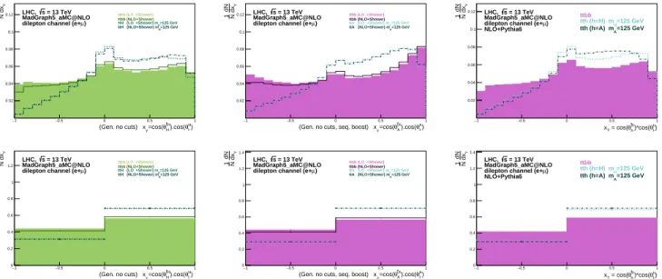
The impact of NLO corrections on the angular distri-butions are shown in Figure 5 (left), by comparing with the LO distributions of xY=cos (θH¯tH) cos (θ`H−), at parton level (including shower effects) without any cuts, both for the SM t¯tH signal and t¯tb¯b background events. NLO (LO) corrections with the impact of shower effects are la-belled NLO+Shower (LO+Shower) through out the text. The same distributions are shown for the t¯tA signal in Figure 5 (middle), with the exception that the sequential prescription was used for the `−. Clear differences are visible between the direct and sequential prescriptions in particular for the background. Figure 5 (right) shows a comparison between t¯tH, t¯tA and t¯tb¯b at NLO+Shower, where the different possible natures of the signal (t¯tH or t¯tA) do not seem to affect significantly the shape of the distribution. In the bottom plots, the correspond-ing distributions with 2 bins are shown, displaycorrespond-ing the differences in forward-backward asymmetries.

t¯tH and t¯tA Signals at NLO+Shower

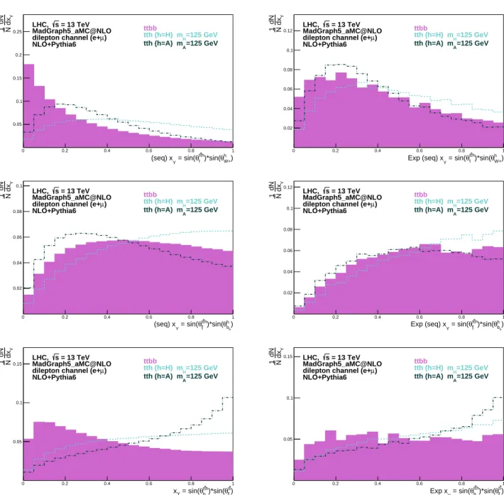
Exploring kinematic differences between t¯tH and t¯tA is of utmost importance in order to find a set of good discriminating variables that may be sensitive to the na-ture of top quark Yukawa coupling. In fact, differences between the scalar and pseudo-scalar are visible through angles between particle directions (t, ¯t and h), already at production. Figure 6 (left) shows, at NLO+Shower, the angle between the top quark and Higgs boson directions (x-axis) versus the angle between the anti-top quark and Higgs boson directions (y-axis), all evaluated in the t¯tH centre-of-mass system. The same distribution is shown for the pseudo-scalar signal t¯tA in Figure 6 (right). In Figure 7, the angle between the top quark direction in the t¯th centre-of-mass frame and the t¯th direction in the lab frame (y-axis), is plotted against the angle between the Higgs direction, in the ¯th rest frame, and the direction of three decay products, all boosted to the h rest frame (x-axis): (left) b quark from Higgs boson, (middle) `+_from

top quark and (right) `− from ¯t. In the top (bottom) row, the t¯tH (t¯tA) signal is shown, without any cuts. Differences between the scalar and pseudo-scalar signals are clearly visible.

Angular Distributions after Reconstruction

Signal distributions are distorted due to cuts from the necessary selection cuts applied to events and the kine-matic fit. The shape of the distributions, although af-fected by the significant reduction on the total number of events, is nevertheless largely preserved. In Figure 8 the same angular distributions as those shown in Figure 7 are

represented, after selection cuts and full kinematic recon-struction. The density of points shows a similar pattern of that from Figure 7. Even after kinematic reconstruc-tion, clear differences between the different signal natures are visible.

Forward-backward asymmetries associated to each of the observables under study, were defined according to [19]

AYF B =

σ(xY > 0) − σ(xY < 0)

σ(xY > 0) + σ(xY < 0)

, (9)

where σ(xY > 0) and σ(xY < 0) correspond to the total

cross section with xY above and below zero, respectively.

The asymmetries are evaluated at NLO+Shower and af-ter the kinematic fit, for different choices of the variable xY (found to provide a significant difference between the

signals and dominant backgound): cos (θ¯th_h) cos (θh_`−) for A

`−(h) F B , b4= (pzt.p z ¯ t)/(|~pt|.|~p¯t|), as defined in [17], for A b4 F B, sin (θt¯th h ) sin (θ ¯ t ¯ bt¯) for A ¯ bt¯(¯t) F B (seq. boost), sin (θt¯th h ) cos (θ ¯ t bh) for A bh(¯t) F B (seq. boost), sin (θt¯th t ) sin (θW +h ) for A W +(h) F B (seq. boost), sin (θt¯¯tth) sin (θ h bh) for A bh(h)

F B (seq. boost) and

sin (θt¯th

h ) sin (θ¯tt¯t) for A ¯ t(t¯t)

F B .

The angular distributions from which each asymmetry was computed are represented in Figures 5 and Figures 9-11. In Table I we show the NLO+Shower values of the asymmetries without any selection applied and after full kinematic reconstruction.

Asymmetries NLO+Shower After selection and

(no cuts applied) reconstruction

t¯tH/t¯tA t¯tb¯b t¯tH/t¯tA t¯tb¯b A`−(h)_{F B} +0.37/+0.41 +0.17 +0.42/+0.39 +0.24 Ab4 F B +0.35/−0.10 +0.33 +0.16/−0.17 +0.12 A¯bt¯(¯t) F B (seq. boost) +0.28/+0.33 −0.17 +0.25/+0.28 +0.03 Abh(¯t) F B (seq. boost) −0.65/−0.77 −0.62 −0.78/−0.83 −0.76 AW +(h)_{F B} (seq. boost) −0.03/−0.46 −0.60 +0.17/−0.06 −0.04 Abh(h) F B (seq. boost) +0.25/−0.08 +0.07 +0.37/+0.16 +0.23 A¯t(t¯_{F B}t) +0.16/+0.37 −0.21 +0.23/+0.31 +0.01

TABLE I: Asymmetry values for t¯tH, t¯tA and t¯tb¯b at

NLO+Shower (without any cuts) and after applying the se-lection criteria and kinematic reconstruction, are shown.

(6)

OBSERVABLES SENSITIVE TO THE CP NATURE OF THE TOP YUKAWA COUPLING

In the previous sections, we identified angular observ-ables for which the distributions of t¯tb¯b events and signal (t¯tH and t¯tA) events show important differences. For many such observables, the distributions of the t¯tH and t¯tA samples are very similar (see the plot on the right of Figure 5 as an example). These observables are ideal to implement a search for (or set limits to) the total t¯th production cross-section, since they have the desirable feature of being insensitive to the CP nature of the Higgs-top coupling. However, within the set of new angular ob-servables, many result in incompatible distributions be-tween t¯tH and t¯tA samples at reconstruction level with-out truth-match. This suggests that they are useful for experimentally measuring (or setting limits to) a pseudo-scalar component of the top Yukawa coupling.

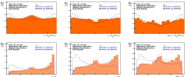
Observables in t¯th events with this same purpose have been previously proposed, for example, in [17, 22, 23]. The observables proposed in these works, for the t¯tH and t¯tA signal samples as well as for the t¯tb¯b background, were studied in reconstructed events. For brevity, we show re-sults for two of the most compelling observables. The authors of [18] proposed the observable β_b¯_b∆θ`h_(`+_{, `}−_),

where θ`h_(`+_{, `}−_{) is the angle between the `}+ _{and `}−

di-rections, projected onto the plane perpendicular to the h direction in the lab frame, and β is defined as the sign of ( ~pb− ~p_b) · ( ~p`− × ~p_`+) (b and ¯b result from the t and ¯t decays, respectively). The other observable is b4, already introduced in the previous section, and first

proposed in [17]. An important remark is that b4, like

many other observables in the referred publications, re-quires the reconstruction of the t and ¯t four-momenta, only achievable through a kinematic fit such as the one used in this work. In Figure 9, distributions are presented of β_b¯_b∆θ`h_(`+_{, `}−_{) (top) and b}

4 (bottom), for t¯tH, t¯tA

and t¯tb¯b samples. They are shown at NLO+Shower with-out cuts (left), with cuts (middle), and at reconstruction level without truth-match, after additionally requiring at least 3 b-tagged jets and |m``− mZ| > 10 GeV (right).

While it is evident that detector simulation and recon-struction degrade the discriminating power of these ob-servables, the most dramatic effect on the distribution shapes comes from applying the acceptance cuts. Af-ter these cuts, the distributions at NLO+Shower already exhibit roughly the same behaviour as the distributions after reconstruction. Optimisation of the selection crite-ria is thus quite important, but stays largely outside the scope of this paper.

In figure 10, distributions of sin (θt¯_hth) sin (θt¯ ¯ bt¯ ) (top) and sin (θt¯th h ) cos (θ ¯ t

bh) (bottom) are shown. These are among the investigated angular observables for which the t¯tb¯b background sample was least compatible with both t¯tH and t¯tA samples. The distributions are represented

at NLO+Shower without cuts (left), after selection cuts (middle), and after full kinematic reconstruction and the additional requirements of |m``− mZ| > 10 GeV and at

least 3 b-tagged jets (right). The dashed line represents the t¯tH distribution and the dashed-dotted line corre-sponds to t¯tA. The shadowed region corresponds to the t¯tb¯b dominant background.

Figure 11 shows distributions of three angular observ-ables among the ones for which the t¯tH and t¯tA samples were least compatible at the reconstruction level with-out truth-match. They are represented at NLO+shower without cuts (left) and at reconstruction level without truth-match, after the previously mentioned cuts on b-tag multiplicity and m`` (right). Distributions of t¯tb¯b

events are also included for completeness. The discrimi-nating performance of these observables is comparable to that of the ones proposed in the literature. Computing the angular observables also requires full reconstruction of t and ¯t. Again, applying the acceptance cuts, detector simulation and kinematic reconstruction visibly degrades the discrimination between t¯tH and t¯tA samples.

ANALYSIS AND RESULTS

In order to estimate the experimental sensitivity of an analysis employing the observables under study, further selection criteria was applied, as mentioned previously. Depletion of the Z+jets background is accomplished by selecting events with a dilepton invariant mass m``such

that |m`+_`−− m_Z| > 10 GeV. This selection was applied in all dilepton flavour categories (ee, µµ and eµ). Most backgrounds, notably t¯t+jets, are then mitigated by se-lecting events with at least 3 b-tagged jets.

Table II shows the expected effective cross-sections in f b, at several levels of the event selection, for dileptonic signal and SM backgrounds. The t¯tA pseudo-scalar sig-nal was scaled to the t¯tH scalar cross-section for compar-ison purposes.

In Figure 12, the expected number of events from the different SM processes are shown, including the Higgs signal, for a luminosity of 100 fb−1at the LHC, for events with at least 3 b-jets (left) and at least 4 b-jets (right). As expected, the composition of backgrounds changes quite significantly after event selection.

The fake data points correspond to one particular pseudo-experiment randomly created from the expected Standard Model t¯tH signal and background distribu-tions. Its purpose is only to guide the reader through the total number of expected events and related statistical uncertainties, after event selection and full reconstruc-tion.

Several kinematic properties of the events, including the new angular distributions introduced in this paper, were tested with several multivariate methods. A boosted decision tree with gradient boost (BDTG) has

(7)

Njets≥ 4 Kinematic mZ Nb Nb

Nlep≥ 2 Fit cut ≥ 3 ≥ 4

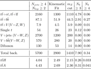
t¯t+c¯c, t¯t+lf 2160 1300 1110 4.78 0.06 t¯t+b¯b 87.1 51.9 44.5 2.91 0.27 t¯t+V (V =Z, W ) 7.9 4.5 3.9 0.09 0.01 Single t 54 26 23 0.12 0.00 V +jets (V =W, Z) 2700 1200 200 0.00 0.00 V +b¯b(V =W, Z) 570 280 20 0.00 0.00 Diboson 130 53 14 0.00 0.00 Total back. 5700 2900 1410 7.90 0.34 t¯tH 4.04 2.49 2.15 0.26 0.033 t¯tA 4.43 2.69 2.36 0.31 0.041

TABLE II: Expected cross-sections (in f b) as a function of selection cuts, at 13 TeV, for dileptonic signal and background events at the LHC.

the best performance among the methods investigated. Its output was used to test the analysis sensitivity to probe the scalar versus pseudo-scalar component of the top-Higgs couplings, as a function of cos α. From the long set of variables tried, the 15 best ranked by the multivariate method, after reconstruc-tion, were: the b4 and Higgs mass (mb¯b); the angular

distributions with direct boost i.e., cos(θ¯th

h ) cos(θh`−), sin(θ_ht¯th) sin(θt¯¯tt) and the variables with sequential

boost sin(θt¯th ¯ t ) sin(θ h bh)(seq.), sin(θ t¯th h ) cos(θ ¯ t bh)(seq.), sin(θt¯th h ) sin(θ ¯ t ¯_b_¯ t)(seq.), sin(θ t¯th

t ) sin(θhW+)(seq.); the ∆η between the jets with maximum ∆η (∆ηmax ∆η_jj ) and the invariant mass of the two b-tagged jets with lowest ∆R

(mmin ∆R_bb ); the ∆R between the Higgs candidate and the

closest (∆Rmin ∆R_hl ) and farthest (∆Rmax ∆R_hl ) leptons; the ∆R between the b-tagged jets with highest pT

(∆Rmax pT

bb ) and the invariant mass of the two jets with

closest value to the Higgs mass (mclosest to 125 GeV_jj ); the jets aplanarity.

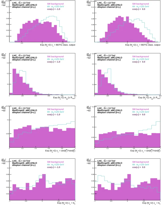
In Figure 13, normalized distributions of the BDTG output classifier (first row) and three of the input vari-ables (remaining rows) used in the multivariate method are shown for the pure scalar (left plots) and pseudo-scalar (right plots) Higgs bosons. It should be noted that the BDTG used for the limit extraction at a given cos(α) has been trained on a signal sample generated with that same value cos(α). This justifies the different SM background shapes between the left and right plots of the first row in Figure 13. The invariant mass of the two b-tagged jets with minimum ∆R (mmin ∆R

bb ) (second

row), the sin(θt¯th h )sin(θ

t¯t ¯

t) (third row) and the b4variable

(fourth row) are also shown for completeness. Shape dif-ferences between signal and background are clearly vis-ible, and they are different for the scalar and

pseudo-scalar cases. In these figures, the line corresponds to the signal distribution and the shaded region corresponds to the full SM background at the LHC.

Expected limits at 95% confidence level (CL) for σ × BR(h → b¯b) and for signal strength µ, in the background-only scenario, were extracted, using the BDTG output distribution. Several signal samples were used, with val-ues of cos(α) ranging from -1 to 1 (in steps of 0.1). Fig-ure 14, first row, shows these limits, for integrated lu-minosities of 100, 300 and 3000 fb−1. Although data taking for large values of luminosity is expected to oc-cur with√s=14 TeV, we show the results at 3000 fb−1

for comparison. Sensitivity to SM t¯tH production at the µ=1 should be attained shortly after the 300 fb−1 mile-stone, using this channel alone. Combining the dileptonic channel with other decay channels should allow to de-crease significantly the luminosity necessary to probe the structure of the top quark Yukawa couplings to the Higgs boson. Figure 14, second and third row, show limits on σ ×BR(h → b¯b) at 300 fb−1, obtained from fits to the fol-lowing individual distributions: sin(θt¯th

h )sin(θt¯¯tt) (center

left), β_b¯_b∆θ`h(`+, `−) (center right); mmin ∆R_bb (bottom left), and b4 (bottom right). The results show that the

different distributions used as input to the BDTG, al-though with the same general dependence on cos(α), can have different sensitivities. A common feature to all vari-ables is a better 95% CL limit on σ × BR(h → b¯b) as we approach the pure pseudo-scalar region. In Figure 15, a comparison is shown between limits on σ × BR(h → b¯b), at 300 fb−1, obtained from each one of the individual dis-tributions used in the BDTG multivariate discriminant. Additionally, the limits corresponding to the BDTG it-self are shown, as well as those from the β_b¯_b∆θ`h_(`+_{, `}−₎

distribution, which is not included in the BDTG, and is only shown for completeness. Figure 15 (left) includes the limits from the angular observables, β_b¯_b∆θ`h_(`+_{, `}−_{), b}

4

and m_b¯_b. Figure 15 (right) shows the limits from all the other individual observables used as input for the BDTG method. The ratios with respect to the limit obtained from the BDTG distribution are also represented. While most individual angular variables result in limits 15 to 20% worse than the BDTG method for the pseudo-scalar case, the other variables tend to be in the 20 to 25% re-gion, with the exception of mmin ∆R

bb , which clearly shows

a better discriminating power (as expected from the plots in Figure 13).

CONCLUSIONS

In this paper, studies of the t¯th production, for scalar and pseudo-scalar Higgs bosons, at a centre-of-mass en-ergy of 13 TeV at the LHC, are considered for differ-ent luminosities. Dileptonic final states from t¯th decays (t → bW+_{→ b`}+_ν

`, ¯t → ¯bW− → ¯b`−ν¯` and h → b¯b) are

(8)

re-constructs the four momenta of the undetected neutrinos. New angular distributions and asymmetries are proposed to allow better discrimination between signals of differ-ent nature (scalar or pseudo-scalar) and backgrounds at the LHC. Using fully reconstructed t¯th events, it is pos-sible to obtain relevant spin information of signal and background processes, through the measurements of new angular distributions and asymmetries. Even after event selection and full kinematical reconstruction, the spin in-formation is largely preserved, opening a window for spin measurements and a better understanding of the nature of the top-Higgs Yukawa coupling and t¯th production at the LHC. Expected limits at 95% CL were extracted on the σ×BR(h → b¯b) and signal strength µ using a boosted decision tree. A comparison between the sensitivities of the individual variables as a function of cos(α) was also performed, showing that a multivariate method combin-ing all the variables can improve the individual limits up to 25%. It should be stressed that some of the angular distributions investigated in this work were used in addi-tion to the kinematical distribuaddi-tions commonly discussed in the literature, yielding at least the same sensitivity to the nature of the top quark Yukawa coupling to Higgs boson, if not better. The fact the expected limits do not exhibit a too strong dependence on the particular choice of the CP-phase (α), makes the analysis of the SM Higgs case (CP-even) a good starting point for any other case, where mixtures with CP-odd contributions are probed. Also, it was found that the invariant mass distribution of the two b-tagged jets with the lowest ∆R between them shows a particularly interesting behaviour. All results presented so far were obtained using the dileptonic final states of t¯th events alone. These are expected to be im-proved when other decay channels are combined, using fully reconstructed final states.

Acknowledgements

This work was partially supported by Fundação para a Ciência e Tecnologia, FCT (projects CERN/FIS-NUC/0005/2015 and CERN/FP/123619/2011, grant SFRH/BPD/100379/2014 and contract IF/01589/2012/CP0180/CT0002). The work of R.S. is supported in part by HARMONIA National Science Center - Poland project UMO-2015/18/M/ST2/00518. The work of R.F. is supported by the Alexander von Humboldt Foundation in the framework of the Sofja Kovalevskaja Award Project “Event Simulation for the Large Hadron Collider at High Precision”. Special thanks goes to our long term collaborator Filipe Veloso for the invaluable help and availability on the evaluation of the confidence limits discussed in this paper.

[1] P. W. Higgs, Phys. Lett. 12, 132 (1964), Phys. Rev. Lett. 13, 508 (1964) and Phys. Rev. 145, 1156 (1964); F. En-glert and R. Brout, Phys. Rev. Lett. 13, 321 (1964); G.S. Guralnik, C.R. Hagen and T.W. Kibble, Phys. Rev. Lett. 13, 585 (1964).

[2] G. Aad et al. [ATLAS Collaboration], Phys. Lett. B 716 (2012) 1, arXiv:1207.7214 [hep-ex];

[3] S. Chatrchyan et al. [CMS Collaboration], Phys. Lett. B 716 (2012) 30, arXiv:1207.7235 [hep-ex];

[4] G. Aad et al. [ATLAS Collaboration], Phys. Lett. B 726 (2013) 88 [Erratum-ibid. B 734 (2014) 406], arXiv:1307.1427 [hep-ex]; G. Aad et al. [ATLAS Collab-oration], Phys. Lett. B 726, 120 (2013), arXiv:1307.1432

[hep-ex]; G. Aad et al. [ATLAS Collaboration],

arXiv:1501.04943 [hep-ex]; V. Khachatryan et al. [CMS Collaboration], arXiv:1412.8662 [hep-ex]; S. Chatrchyan et al. [CMS Collaboration], Nature Phys. 10, 557 (2014) arXiv:1401.6527 [hep-ex];

[5] D. Fontes, J. C. Romão, R. Santos and J. P. Silva, JHEP 1506, 060 (2015) doi:10.1007/JHEP06(2015)060 [arXiv:1502.01720 [hep-ph]].

[6] V. Khachatryan et al. [CMS Collaboration],

arXiv:1411.3441 [hep-ex].

[7] V. Khachatryan et al. [CMS Collaboration], Phys. Lett. B 759, 672 (2016) doi:10.1016/j.physletb.2016.06.004 [arXiv:1602.04305 [hep-ex]].

[8] G. Aad et al. [ATLAS Collaboration], Eur. Phys. J. C 75, no. 10, 476 (2015) Erratum: [Eur. Phys. J. C 76, no. 3, 152 (2016)] doi:10.1140/epjc/s10052-015-3685-1, 10.1140/epjc/s10052-016-3934-y [arXiv:1506.05669 [hep-ex]].

[9] J. N. Ng and P. Zakarauskas, Phys. Rev. D 29, 876 (1984); Z. Kunszt, Nucl. Phys. B 247, 339 (1984); W. J. Marciano and F. E. Paige, Phys. Rev. Lett. 66, 2433 (1991); J. F. Gunion, Phys. Lett. B 261, 510 (1991); J. Goldstein et al., Phys. Rev. Lett. 86, 1694 (2001), [hep-ph/0006311]; W. Beenakker et al., Phys. Rev. Lett. 87, 201805 (2001), [hep-ph/0107081] and Nucl. Phys. B 653, 151 (2003), [hep-ph/0211352]; L. Reina and S. Dawson, Phys. Rev. Lett. 87, 201804 (2001), [hep-ph/0107101]; S. Dawson et al., Phys. Rev. D 67, 071503 (2003), [hep-ph/0211438]; S. Dawson et al., Phys. Rev. D 68, 034022 (2003) [hep-ph/0305087]; S. Dittmaier, M. Kramer, and M. Spira, Phys. Rev. D 70, 074010 (2004) [hep-ph/0309204]; R. Frederix et al., Phys. Lett. B 701, 427 (2011) [arXiv:1104.5613 [hep-ph]]; M. V. Garzelli et al., Europhys. Lett. 96 (2011) 11001 [arXiv:1108.0387 [hep-ph]]; H. B. Hartanto et al., arXiv:1501.04498 [hep-ph]; S. Frixione, V. Hirschi, D. Pa-gani, H. S. Shao and M. Zaro, JHEP 1409 (2014) 065 [arXiv:1407.0823 [hep-ph]]; Y. Zhang, W. G. Ma, R. Y. Zhang, C. Chen and L. Guo, Phys. Lett. B 738 (2014) 1 [arXiv:1407.1110 [hep-ph]].

[10] G. Aad et al. [ATLAS Collaboration], JHEP 1605, 160 (2016) doi:10.1007/JHEP05(2016)160 [arXiv:1604.03812 [hep-ex]].

[11] G. Aad et al. [ATLAS Collaboration] Phys. Lett. B 740 (2015) 222, arXiv:1409.3122 [hep-ex].

[12] G. Aad et al. [ATLAS Collaboration], Phys. Lett. B 749, 519 (2015) doi:10.1016/j.physletb.2015.07.079 [arXiv:1506.05988 [hep-ex]].

(9)

[13] G. Aad et al. [ATLAS Collaboration], arXiv:1503.05066 [hep-ex].

JHEP 1409, 087 (2014) Erratum: [JHEP

1410, 106 (2014)] doi:10.1007/JHEP09(2014)087,

10.1007/JHEP10(2014)106 [arXiv:1408.1682 [hep-ex]].

arXiv:1502.02485 [hep-ex].

[16] G. Aad et al. [ATLAS and CMS Collaborations], JHEP 1608, 045 (2016) doi:10.1007/JHEP08(2016)045 [arXiv:1606.02266 [hep-ex]].

[17] J. F. Gunion and X. G. He, Phys. Rev. Lett.

76 (1996) 4468 doi:10.1103/PhysRevLett.76.4468 [hep-ph/9602226].

[18] F. Boudjema, R. M. Godbole, D. Guadagnoli and K. A. Mohan, arXiv:1501.03157 [hep-ph];

[19] S. P. A. dos Santos, J. P. Araque, R. Cantrill, N. F. Cas-tro, M. C. N. Fiolhais, R. Frederix, R. Gonçalo and R. Martins et al., Phys. Rev. D 92, 034021 (2015), arXiv:1503.07787 [hep-ph].

[20] S. Berge, W. Bernreuther and S. Kirchner, Eur. Phys. J. C 74, no. 11, 3164 (2014), arXiv:1408.0798 [hep-ph]; S. Berge, W. Bernreuther and H. Spiesberger, arXiv:1208.1507 [hep-ph]; S. Berge, W. Bernreuther, B. Niepelt and H. Spiesberger, Phys. Rev. D 84,

116003 (2011), arXiv:1108.0670 [hep-ph]; S. Berge,

W. Bernreuther and J. Ziethe, Phys. Rev. Lett. 100, 171605 (2008), arXiv:0801.2297 [hep-ph]; S. Khatibi and M. M. Najafabadi, Phys. Rev. D 90 (2014) 7, 074014 [arXiv:1409.6553 [hep-ph]].

[21] [21] G. Brooijmans et al., arXiv:1405.1617 [hep-ph]. [22] J. Ellis et al., JHEP 1404, 004 (2014) [arXiv:1312.5736

[hep-ph]]; S. Biswas et al., JHEP 1407, 020 (2014) [arXiv:1403.1790 [hep-ph]]; F. Demartin et al., Eur. Phys. J. C 74, no. 9, 3065 (2014) [arXiv:1407.5089 [hep-ph]];

[23] P. Artoisenet et al., JHEP 1303, 015 (2013),

arXiv:1212.3460 [hep-ph].

[24] J. Alwall et al., JHEP 1407, 079 (2014), arXiv:1405.0301 [hep-ph].

[25] R. D. Ball et al., Nucl. Phys. B 867, 244 (2013) [arXiv:1207.1303 [hep-ph]].

[26] P. Artoisenet et al., JHEP 1311 (2013) 043

doi:10.1007/JHEP11(2013)043 [arXiv:1306.6464

[hep-ph]].

[27] M. Czakon and A. Mitov, Comput. Phys.

Com-mun. 185 (2014) 2930 doi:10.1016/j.cpc.2014.06.021 [arXiv:1112.5675 [hep-ph]].

[28] M. Botje et al., arXiv:1101.0538 [hep-ph].

[29] A. D. Martin, W. J. Stirling, R. S. Thorne and G. Watt, Eur. Phys. J. C 64, 653 (2009) [arXiv:0905.3531 [hep-ph]].

[30] J. Gao et al., Phys. Rev. D 89, no. 3, 033009 (2014) [arXiv:1302.6246 [hep-ph]].

[31] N. Kidonakis, Phys. Rev. D 81, 054028 (2010)

[arXiv:1001.5034 [hep-ph]].

[32] N. Kidonakis, Phys. Rev. D 83, 091503 (2011)

[arXiv:1103.2792 [hep-ph]].

[33] M. Czakon, P. Fiedler and A. Mitov, Phys. Rev. Lett. 110, 252004 (2013) arXiv:1303.6254 [hep-ph].

[34] T. Sjostrand, S. Mrenna and P. Z. Skands, JHEP 0605, 026 (2006), hep-ph/0603175.

[35] J. Alwall et al., Eur. Phys. J. C 53 (2008) 473

doi:10.1140/epjc/s10052-007-0490-5 [arXiv:0706.2569

[hep-ph]].

[36] S. Frixione and B. R. Webber, JHEP 0206 (2002) 029 doi:10.1088/1126-6708/2002/06/029 [hep-ph/0204244] [37] J. de Favereau et al. [DELPHES 3 Collaboration], JHEP

1402, 057 (2014), arXiv:1307.6346 [hep-ex].

[38] M. Cacciari, G. P. Salam and G. Soyez, JHEP

0804 (2008) 063 doi:10.1088/1126-6708/2008/04/063 [arXiv:0802.1189 [hep-ph]].

[39] E. Conte, B. Fuks and G. Serret, Comput. Phys. Com-mun. 184, 222 (2013), arXiv:1206.1599 [hep-ph]. [40] E. Conte et al., Eur. Phys. J. C 74, no. 10, 3103 (2014),

arXiv:1405.3982 [hep-ph].

[41] A. Hoecker, P. Speckmayer, J. Stelzer, J. Therhaag, E. von Toerne, and H. Voss, “TMVA: Toolkit for Multivariate Data Analysis,” PoS A CAT 040 (2007) [physics/0703039].

(10)

) t R(l+,b ∆ 1 2 3 4 5 6 0.116 / (1/N) dN 0 0.1 0.2 0.3 0.4 0.5 0.6 0.7 _Signal Background U/O-flow (S,B): (0.0, 0.0)% / (0.0, 0.0)% ) t R(l+,b ∆ Input variable: ) t (l+,b θ ∆ 0.5 1 1.5 2 2.5 3 0.0623 / (1/N) dN 0 0.1 0.2 0.3 0.4 0.5 0.6 0.7 U/O-flow (S,B): (0.0, 0.0)% / (0.0, 0.0)% ) t (l+,b θ ∆ Input variable: ) t (l+,b Φ ∆ 3 − −2 −1 0 1 2 3 0.128 / (1/N) dN 0 0.05 0.1 0.15 0.2 0.25 U/O-flow (S,B): (0.0, 0.0)% / (0.0, 0.0)% ) t (l+,b Φ ∆ Input variable: ) H b , H R(b ∆ 1 2 3 4 5 6 0.121 / (1/N) dN 0 0.1 0.2 0.3 0.4 0.5 U/O-flow (S,B): (0.0, 0.0)% / (0.0, 0.0)% ) H b , H R(b ∆ Input variable: ) H b , H (b θ ∆ 0.5 1 1.5 2 2.5 3 0.0627 / (1/N) dN 0 0.1 0.2 0.3 0.4 0.5 0.6 U/O-flow (S,B): (0.0, 0.0)% / (0.0, 0.0)% ) H b , H (b θ ∆ Input variable: ) H b , H (b Φ ∆ 3 − −2 −1 0 1 2 3 0.128 / (1/N) dN 0 0.02 0.04 0.06 0.08 0.1 0.12 0.14 0.16 0.18 0.2 0.22 U/O-flow (S,B): (0.0, 0.0)% / (0.0, 0.0)% ) H b , H (b Φ ∆ Input variable:

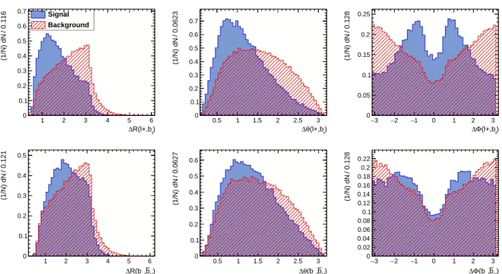
FIG. 1: Distributions of TMVA input variables for right (filled blue, labelled "Signal") and wrong combinations (red shaded,

labelled "Background") of jets and leptons from the same parent decaying particle: ∆R(`+, bt) (top left) and ∆R(bH, ¯bH)

(bottom left); ∆θ(`+, bt) (top middle) and ∆θ(bH, ¯bH) (bottom middle); ∆Φ(`+, bt) (top right) and ∆Φ(bH, ¯bH) (bottom

right), see text for details.

)[GeV] t m(l+,b 100 200 300 400 500 600 13.2 / (1/N) dN 0 0.002 0.004 0.006 0.008 0.01 0.012 0.014 U/O-flow (S,B): (0.0, 0.0)% / (0.0, 0.1)% )[GeV] t Input variable: m(l+,b BDT response 0.4 − −0.2 0 0.2 0.4 dx / (1/N) dN 0 1 2 3 4 5 6

7 _{Signal (test sample)}

Background (test sample)

Signal (training sample) Background (training sample) Kolmogorov-Smirnov test: signal (background) probability = 0.019 ( 0.14)

U/O-flow (S,B): (0.0, 0.0)% / (0.0, 0.0)%

TMVA overtraining check for classifier: BDT

100 − 80 − 60 − 40 − 20 − 0 20 40 60 80 100 ) t R(l+,b ∆ ) t b R(l-, ∆ ) H b , H R(b ∆ ) t (l+,b Φ ∆ ) t b (l-, Φ ∆ ) H b , H (b Φ ∆ ) t (l+,b θ ∆ ) t b (l-, θ ∆ ) H b , H (b θ ∆ )[GeV] t m(l+,b )[GeV] t b m(l-, )[GeV] H b , H (b rec m ) t R(l+,b ∆ ) t b R(l-, ∆ ) H b , H R(b ∆ ) t (l+,b Φ ∆ ) t b (l-, Φ ∆ ) H b , H (b Φ ∆ ) t (l+,b θ ∆ ) t b (l-, θ ∆ ) H b , H (b θ ∆ )[GeV] t m(l+,b )[GeV] t b m(l-, )[GeV] H b , H (b rec m

Correlation Matrix (signal)

100 13 12 -1 69 9 9 34 -1 13 100 11 9 69 8 -1 35 -2 12 11 100 10 9 63 -1 13 -1 100 -2 -1 -2 100 -1 100 69 9 10 -1 100 7 13 27 9 69 9 7 100 13 28 -1 9 8 63 -1 13 13 100 10 34 -1 27 100 35 -1 28 100 -1 -1 -2 13 -1 10 -1 100 Linear correlation coefficients in %

)[GeV] H b , H (b rec m 100 200 300 400 500 600 700 800 16.2 / (1/N) dN 0 0.002 0.004 0.006 0.008 0.01 0.012 0.014 0.016 0.018 0.02 U/O-flow (S,B): (0.0, 0.0)% / (0.0, 0.0)% )[GeV] H b , H (b rec Input variable: m BDTG response 1 − −0.8 −0.6 −0.4 −0.2 0 0.2 0.4 0.6 0.8 dx / (1/N) dN 0 2 4 6 8 10 12

Signal (test sample) Background (test sample)

Signal (training sample) Background (training sample) Kolmogorov-Smirnov test: signal (background) probability = 0.082 ( 0.14)

U/O-flow (S,B): (0.0, 0.0)% / (0.0, 0.0)%

TMVA overtraining check for classifier: BDTG

100 − 80 − 60 − 40 − 20 − 0 20 40 60 80 100 ) t R(l+,b ∆ ) t b R(l-, ∆ ) H b , H R(b ∆ ) t (l+,b Φ ∆ ) t b (l-, Φ ∆ ) H b , H (b Φ ∆ ) t (l+,b θ ∆ ) t b (l-, θ ∆ ) H b , H (b θ ∆ )[GeV] t m(l+,b )[GeV] t b m(l-, )[GeV] H b , H (b rec m ) t R(l+,b ∆ ) t b R(l-, ∆ ) H b , H R(b ∆ ) t (l+,b Φ ∆ ) t b (l-, Φ ∆ ) H b , H (b Φ ∆ ) t (l+,b θ ∆ ) t b (l-, θ ∆ ) H b , H (b θ ∆ )[GeV] t m(l+,b )[GeV] t b m(l-, )[GeV] H b , H (b rec m

Correlation Matrix (background)

100 2 4 71 2 4 59 1 2 2 100 3 1 71 3 59 1 4 3 100 3 3 70 2 1 60 100 2 -3 2 100 -3 100 71 1 3 100 11 12 46 1 2 2 71 3 11 100 12 1 47 1 4 3 70 12 12 100 3 3 47 59 2 46 1 3100 3 5 1 59 1 1 47 3 3 100 4 2 1 60 2 1 47 5 4 100 Linear correlation coefficients in %

FIG. 2: Mass distributions (left) for right (filled blue, signal) and wrong (red shaded, background) combinations of jets and

leptons from the same parent decaying particle: (upper-left) the m(`+, bt) and (lower-left) m(bH, ¯bH); (middle-top) BDT and

(middle-bottom) BDTG TMVA methods response for signal and background; (right-top) TMVA input variables correlations for signal and (right-bottom) background.

(11)

0.0002 0.0004 0.0006 0.0008 0.001 0.0012 0.0014 0.0016 (W+) [GeV] T (NLO+Shower) P 0 50 100 150 200 250 300 350 400 (W+) [GeV] T

(rec. w/o truth match) P

0 50 100 150 200 250 300 350 400 = 13 TeV s LHC, MadGraph5_aMC@NLO 2 ) T N(dP N 2 d =125 GeV H H events, m t t ) µ dilepton channel (e+

0.1 0.2 0.3 0.4 0.5 0.6 0.7 3 − 10 × (t) [GeV] T (NLO+Shower) P 0 50 100 150 200 250 300 350 400 (t) [GeV] T

0.0002 0.0004 0.0006 0.0008 0.001 0.0012 0.0014 ) [GeV] t (t T (NLO+Shower) P 0 50 100 150 200 250 300 350 400 ) [GeV]t (tT

0.0002 0.0004 0.0006 0.0008 0.001 0.0012 0.0014 0.0016 0.0018 0.002 (h) [GeV] T (NLO+Shower) P 0 50 100 150 200 250 300 350 400 (h) [GeV] T

FIG. 3: Two-dimensional distributions of pT in t¯tH events. The horizontal axes represent variables recorded at NLO+Shower,

and the vertical axes represent the corresponding variables recorded at reconstruction level without truth-match. Upper-left:

distribution for W+. A similar distribution is obtained for W−, but is not shown here. Upper-right: distribution for t. A

similar distribution is obtained for ¯t, but is not shown here. Lower-left: distribution for t¯t. Lower-right: distribution for H.

0.05 0.1 0.15 0.2 0.25 0.3 0.35 0.4 0.45 3 − 10 × ) [GeV] l ν ( T (NLO+Shower) P 0 10 20 30 40 50 60 70 80 90 100 ) [GeV]l ν ( T

0 10 20 30 40 50 60 70 80 90 100 = 13 TeV s LHC, MadGraph5_aMC@NLO 2 ) T N(dP N 2 d =125 GeV H H events, m t t ) µ dilepton channel (e+

[GeV] H m 50 100 150 200 dm dN N 1 0.005 0.01 0.015 0.02 0.025 0.03 0.035 0.04 0.045 = 13 TeV s pp @ MadGraph5_aMC@NLO

H (rec. w/o truth-match) t

t

FIG. 4: Two-dimensional distribution of the neutrino pT in t¯tH events (left): the NLO+Shower pT (x-axis) against the

reconstructed pT without match (y-axis) is shown. Distribution of the reconstructed Higgs boson mass without

(12)

) l-H θ ).cos( H H t θ =cos( Y (Gen. no cuts) x 1 − −0.5 0 0.5 1 Y dx dN N 1 0.02 0.04 0.06 0.08 0.1 0.12 LHC, s = 13 TeV

MadGraph5_aMC@NLO ttbb (LO +Shower)ttbb (NLO+Shower)

=125 GeV H ttH (LO +Shower) m =125 GeV H ttH (NLO+Shower) m ) µ

dilepton channel (e+

) l-A θ ).cos( A A t θ =cos( Y

(Gen. no cuts, seq. boost) x

1 − −0.5 0 0.5 1 Y dx dN N 1 0.02 0.04 0.06 0.08 0.1 0.12 LHC, s = 13 TeV

MadGraph5_aMC@NLO ttbb (LO +Shower)ttbb (NLO+Shower) =125 GeV A ttA (LO +Shower) m

=125 GeV

A

ttA (NLO+Shower) m

)

µ

) l-h θ )*cos( h h t θ = cos( Y x 1 − −0.5 0 0.5 1 Y dx dN N 1 0.02 0.04 0.06 0.08 0.1 0.12 LHC, s = 13 TeV MadGraph5_aMC@NLO NLO+Pythia6 ttbb =125 GeV H tth (h=H) m =125 GeV A tth (h=A) m ) µ

) l-H θ ).cos( H H t θ =cos( Y (Gen. no cuts) x 1 − −0.5 0 0.5 1 Y dx dN N 1 0 0.2 0.4 0.6 0.8 1 1.2 = 13 TeV s LHC,

MadGraph5_aMC@NLO ttbb (LO +Shower)ttbb (NLO+Shower)

=125 GeV H ttH (LO +Shower) m =125 GeV H ttH (NLO+Shower) m ) µ

) l-A θ ).cos( A A t θ =cos( Y

(Gen. no cuts, seq. boost) x

1 − −0.5 0 0.5 1 Y dx dN N 1 0 0.2 0.4 0.6 0.8 1 1.2 1.4 = 13 TeV s LHC,

MadGraph5_aMC@NLO ttbb (LO +Shower)ttbb (NLO+Shower) =125 GeV A ttA (LO +Shower) m

=125 GeV

A

ttA (NLO+Shower) m

)

µ

) l-h θ )*cos( h h t θ = cos( Y x 1 − −0.5 0 0.5 1 Y dx dN N 1 0 0.2 0.4 0.6 0.8 1 1.2 1.4 = 13 TeV s LHC, MadGraph5_aMC@NLO NLO+Pythia6 ttbb =125 GeV H tth (h=H) m =125 GeV A tth (h=A) m ) µ

FIG. 5: NLO+Shower versus LO+Shower behaviour of the distribution of xY=cos (θ¯tHH ) cos (θ

H

`−) at parton Level with shower

effects, without any selection cuts nor reconstruction, for the SM signal t¯tH (left) and for the t¯tA signal (middle), each one

against the main background t¯tb¯b. Notice that, for the middle plots, the sequential boost prescription was employed for the

lepton. The differences between the LO+Shower and NLO+Shower angular distributions are shown on top. Asymmetries

around xY = 0 are visible in the 2 binned distributions (bottom). The t¯tH, t¯tA and t¯tb¯b angular distributions at NLO are

compared (top right), and the corresponding 2 binned distributions show the asymmetries (bottom right).

0.0002 0.0004 0.0006 0.0008 0.001 0.0012 0.0014 0.0016 0.0018 ,H) t ( H t t θ ∆ 0 0.5 1 1.5 2 2.5 3 (t,H) Ht t θ∆ 0 1 2 3 = 13 TeV s LHC, MadGraph5_aMC@NLO =125 GeV H H events, m t t ) µ

0.0002 0.0004 0.0006 0.0008 0.001 0.0012 ,A) t ( A t t θ ∆ 0 0.5 1 1.5 2 2.5 3 (t,A) At t θ∆ 0 1 2 3 = 13 TeV s LHC, MadGraph5_aMC@NLO =125 GeV A A events, m t t ) µ

FIG. 6: Angle between the t quark and Higgs boson (x-axis) at NLO+Shower effects plotted against the angle between the ¯t

quark and Higgs boson (y-axis), in the t¯tH centre-of-mass system. The SM Higss boson (H) distribution (left) and the pure

(13)

0.05 0.1 0.15 0.2 0.25 0.3 0.35 0.4 0.45 3 − 10 × H b H θ 0 0.5 1 1.5 2 2.5 3 t Ht t_θ 0 1 2 3 = 13 TeV s LHC, MadGraph5_aMC@NLO =125 GeV H H events, m t t ) µ

0.1 0.2 0.3 0.4 0.5 0.6 3 − 10 × l+ H θ 0 0.5 1 1.5 2 2.5 3 t Ht t_θ 0 1 2 3 = 13 TeV s LHC, MadGraph5_aMC@NLO =125 GeV H H events, m t t ) µ

0.0002 0.0004 0.0006 0.0008 0.001 l-H θ 0 0.5 1 1.5 2 2.5 3 t Ht t_θ 0 1 2 3 = 13 TeV s LHC, MadGraph5_aMC@NLO =125 GeV H H events, m t t ) µ

0.05 0.1 0.15 0.2 0.25 0.3 0.35 0.4 0.45 3 − 10 × A b A θ 0 0.5 1 1.5 2 2.5 3 t At t_θ 0 1 2 3 = 13 TeV s LHC, MadGraph5_aMC@NLO =125 GeV A A events, m t t ) µ

0.1 0.2 0.3 0.4 0.5 0.6 3 − 10 × l+ A θ 0 0.5 1 1.5 2 2.5 3 t At t_θ 0 1 2 3 = 13 TeV s LHC, MadGraph5_aMC@NLO =125 GeV A A events, m t t ) µ

0.0002 0.0004 0.0006 0.0008 0.001 0.0012 0.0014 0.0016 l-A θ 0 0.5 1 1.5 2 2.5 3 t At t_θ 0 1 2 3 = 13 TeV s LHC, MadGraph5_aMC@NLO =125 GeV A A events, m t t ) µ

FIG. 7: Two dimensional distribution at NLO+Shower of the angle between the top quark, in the t¯th centre-of-mass frame,

and the t¯th direction in the lab frame (y-axis) plotted against the angle between the Higgs direction, in the ¯th rest frame, and

the direction of several decay products (all boosted to the Higgs centre-of-mass): (left) b quark from h, (middle) `+ from top

quark and (right) `−from ¯t. The top (bottom) distributions correspond to t¯tH (t¯tA), without any cuts.

0.0001 0.0002 0.0003 0.0004 0.0005 0.0006 0.0007 0.0008 0.0009 0.001 H b H θ Exp 0 0.5 1 1.5 2 2.5 3 t Ht t_θ Exp 0 1 2 3 = 13 TeV s LHC, MadGraph5_aMC@NLO =125 GeV H H events, m t t ) µ

0.0002 0.0004 0.0006 0.0008 0.001 0.0012 l+ H θ Exp 0 0.5 1 1.5 2 2.5 3 t Ht t_θ Exp 0 1 2 3 = 13 TeV s LHC, MadGraph5_aMC@NLO =125 GeV H H events, m t t ) µ

0.0002 0.0004 0.0006 0.0008 0.001 0.0012 0.0014 0.0016 0.0018 0.002 l-H θ Exp 0 0.5 1 1.5 2 2.5 3 t Ht t_θ Exp 0 1 2 3 = 13 TeV s LHC, MadGraph5_aMC@NLO =125 GeV H H events, m t t ) µ

0.1 0.2 0.3 0.4 0.5 0.6 0.7 0.8 3 − 10 × A b A θ Exp 0 0.5 1 1.5 2 2.5 3 t Att θ Exp 0 1 2 3 = 13 TeV s LHC, MadGraph5_aMC@NLO =125 GeV A A events, m t t ) µ

0.0002 0.0004 0.0006 0.0008 0.001 l+ A θ Exp 0 0.5 1 1.5 2 2.5 3 t Att θ Exp 0 1 2 3 = 13 TeV s LHC, MadGraph5_aMC@NLO =125 GeV A A events, m t t ) µ

0.0002 0.0004 0.0006 0.0008 0.001 0.0012 0.0014 0.0016 0.0018 0.002 l-A θ Exp 0 0.5 1 1.5 2 2.5 3 t Att θ Exp 0 1 2 3 = 13 TeV s LHC, MadGraph5_aMC@NLO =125 GeV A A events, m t t ) µ

(14)

(l+,l-) lh θ ∆ b b β = Y x 2 − 0 2 Y dx dN N 1 0.02 0.04 0.06 0.08 0.1 = 13 TeV s LHC, MadGraph5_aMC@NLO NLO+Pythia6 ttbb =125 GeV H tth (h=H) m =125 GeV A tth (h=A) m ) µ

(l+,l-) lh θ ∆ b b β = Y x 2 − 0 2 Y dx dN N 1 0.02 0.04 0.06 0.08 0.1 LHC, s = 13 TeV MadGraph5_aMC@NLO NLO+Pythia6 ttbb =125 GeV H tth (h=H) m =125 GeV A tth (h=A) m ) µ

(l+,l-) lh θ ∆ b b β = Y Exp x 2 − 0 2 Y dx dN N 1 0.02 0.04 0.06 0.08 0.1 0.12 _LHC,_s_{= 13 TeV} MadGraph5_aMC@NLO NLO+Pythia6 ttbb =125 GeV H tth (h=H) m =125 GeV A tth (h=A) m ) µ

4 = b Y x 1 − −0.5 0 0.5 1 Y dx dN N 1 0.05 0.1 0.15 0.2 0.25 = 13 TeV s LHC, MadGraph5_aMC@NLO NLO+Pythia6 ttbb =125 GeV H tth (h=H) m =125 GeV A tth (h=A) m ) µ

4 = b Y x 1 − −0.5 0 0.5 1 Y dx dN N 1 0.02 0.04 0.06 0.08 0.1 0.12 0.14 = 13 TeV s LHC, MadGraph5_aMC@NLO NLO+Pythia6 ttbb =125 GeV H tth (h=H) m =125 GeV A tth (h=A) m ) µ

4 = b Y Exp x 1 − −0.5 0 0.5 1 Y dx dN N 1 0.02 0.04 0.06 0.08 0.1 0.12 = 13 TeV s LHC, MadGraph5_aMC@NLO NLO+Pythia6 ttbb =125 GeV H tth (h=H) m =125 GeV A tth (h=A) m ) µ

FIG. 9: Normalised β∆θ`h_{(`+, `−) distributions at NLO+Shower without cuts (top left), with cuts (top middle) and after}

cuts and full kinematic reconstruction (top right). The NLO+Shower b4 distribution is also shown at parton level without cuts

(bottom left), with cuts (bottom middle) and after cuts and full kinematic reconstruction (bottom right). The dashed line

represents the t¯th SM model signal (h = H and CP = +1) and the dashed-dotted line corresponds to the pure pseudo-scalar

distribution t¯th (h = A and CP = −1). The shadowed region corresponds to the NLO+Shower t¯tb¯b dominant background.

) t b t θ )*sin( h h t t θ = sin( Y (seq) x 0 0.2 0.4 0.6 0.8 1 Y dx dN N 1 0.02 0.04 0.06 0.08 0.1 0.12 = 13 TeV s LHC, MadGraph5_aMC@NLO NLO+Pythia6 ttbb =125 GeV H tth (h=H) m =125 GeV A tth (h=A) m ) µ

) t b t θ )*sin( h h t t θ = sin( Y (seq) x 0 0.2 0.4 0.6 0.8 1 Y dx dN N 1 0.02 0.04 0.06 0.08 0.1 0.12 LHC, s = 13 TeV MadGraph5_aMC@NLO NLO+Pythia6 ttbb =125 GeV H tth (h=H) m =125 GeV A tth (h=A) m ) µ

) t b t θ )*sin( h h t t θ = sin( Y Exp (seq) x 0 0.2 0.4 0.6 0.8 1 Y dx dN N 1 0.02 0.04 0.06 0.08 0.1 LHC, s = 13 TeV MadGraph5_aMC@NLO NLO+Pythia6 ttbb =125 GeV H tth (h=H) m =125 GeV A tth (h=A) m ) µ

) h b t θ )*cos( h h t t θ = sin( Y (seq) x 1 − −0.5 0 0.5 1 Y dx dN N 1 0.05 0.1 0.15 0.2 _LHC,_s_{= 13 TeV} MadGraph5_aMC@NLO NLO+Pythia6 ttbb =125 GeV H tth (h=H) m =125 GeV A tth (h=A) m ) µ

) h b t θ )*cos( h h t t θ = sin( Y (seq) x 1 − −0.5 0 0.5 1 Y dx dN N 1 0.05 0.1 0.15 0.2 LHC, s = 13 TeV MadGraph5_aMC@NLO NLO+Pythia6 ttbb =125 GeV H tth (h=H) m =125 GeV A tth (h=A) m ) µ

) h b t θ )*cos( h h t t θ = sin( Y Exp (seq) x 1 − −0.5 0 0.5 1 Y dx dN N 1 0.05 0.1 0.15 0.2 = 13 TeV s LHC, MadGraph5_aMC@NLO NLO+Pythia6 ttbb =125 GeV H tth (h=H) m =125 GeV A tth (h=A) m ) µ

FIG. 10: Distributions of xY=sin (θht¯th) sin (θ

¯ t ¯

bt¯) (top) and xY=sin (θ

t¯th

h ) cos (θ

¯ t

bh) (bottom). The distributions at NLO+Shower

(left), after cuts (middle) and after cuts and full kinematic reconstruction (right), are shown. The dashed line represents the

t¯th SM model signal (h = H and CP = +1) and the dashed-dotted line corresponds to the pure pseudo-scalar distribution t¯th

(h = A and CP = −1). The shadowed region corresponds to the NLO+Shower t¯tb¯b dominant background. The laboratory

(15)

) W+ h θ )*sin( t h t t θ = sin( Y (seq) x 0 0.2 0.4 0.6 0.8 1 Y dx dN N 1 0.05 0.1 0.15 0.2 0.25 = 13 TeV s LHC, MadGraph5_aMC@NLO NLO+Pythia6 ttbb =125 GeV H tth (h=H) m =125 GeV A tth (h=A) m ) µ

) W+ h θ )*sin( t h t t θ = sin( Y Exp (seq) x 0 0.2 0.4 0.6 0.8 1 Y dx dN N 1 0.02 0.04 0.06 0.08 0.1 0.12 = 13 TeV s LHC, MadGraph5_aMC@NLO NLO+Pythia6 ttbb =125 GeV H tth (h=H) m =125 GeV A tth (h=A) m ) µ

) h b h θ )*sin( t h t t θ = sin( Y (seq) x 0 0.2 0.4 0.6 0.8 1 Y dx dN N 1 0.02 0.04 0.06 0.08 0.1 = 13 TeV s LHC, MadGraph5_aMC@NLO NLO+Pythia6 ttbb =125 GeV H tth (h=H) m =125 GeV A tth (h=A) m ) µ

) h b h θ )*sin( t h t t θ = sin( Y Exp (seq) x 0 0.2 0.4 0.6 0.8 1 Y dx dN N 1 0.02 0.04 0.06 0.08 0.1 0.12 = 13 TeV s LHC, MadGraph5_aMC@NLO NLO+Pythia6 ttbb =125 GeV H tth (h=H) m =125 GeV A tth (h=A) m ) µ

) t t t θ )*sin( h h t t θ = sin( Y x 0 0.2 0.4 0.6 0.8 1 Y dx dN N 1 0.05 0.1 0.15 = 13 TeV s LHC, MadGraph5_aMC@NLO NLO+Pythia6 ttbb =125 GeV H tth (h=H) m =125 GeV A tth (h=A) m ) µ

) t t t θ )*sin( h h t t θ = sin( Y Exp x 0 0.2 0.4 0.6 0.8 1 Y dx dN N 1 0.05 0.1 0.15 _LHC, _s_{= 13 TeV} MadGraph5_aMC@NLO NLO+Pythia6 ttbb =125 GeV H tth (h=H) m =125 GeV A tth (h=A) m ) µ

FIG. 11: NLO+Shower angular distributions at parton level before selection cuts (left) and after all cuts and full kinematic

reconstruction (right) of: (top) xY=sin (θtt¯tH) sin (θW +H ), (middle) xY=sin (θt¯¯ttH) sin (θ

H

bH) and (bottom) xY=sin (θ

t¯tH

H ) sin (θtt¯¯t).

The dashed line represents the t¯th SM model signal (h = H and CP = +1), the dashed-dotted line corresponds to the pure

pseudo-scalar distribution t¯th (h = A and CP = −1) and the shadowed region corresponds to the NLO+Shower t¯tb¯b dominant