MODELLING AIR TEMPERATURE IN BRAZILIAN NORTHEAST TO EVALUATE CHANGE PATTERNS FROM 2000 TO 2017
Daniel Moraes1 Dr. Sara Ribeiro1 Dr. Ana Cristina Costa1
1Nova Information Management School (NOVA IMS), Universidade Nova de Lisboa, Portugal ABSTRACT
Air temperature influences a variety of environmental processes, having a significant impact on the conditions of living of humans and other life forms. The Brazilian Northeast is a region that comprises a diversity of ecosystems, but it is most known as a semi-arid area characterized by severe environmental conditions. This work proposes to model air temperature in Brazilian Northeast to evaluate changing patterns between 2000 and 2017 using two interpolation techniques and comparing them. Monthly average temperature data from meteorological stations were gathered and used to compute the average annual temperature. Then, the timeframe was divided into 2 periods: 2000 to 2008 (1) and 2009 to 2017 (2), and the average temperature of each period was computed based on the annual average. Descriptive statistics analysis and exploratory spatial data analysis were performed, providing insights on the temperature patterns and distribution. In addition, interpolated surfaces were generated using the Inverse Distance Weighting and Ordinary Kriging methods for each period, and results were compared using error statistics derived with cross-validation. The results revealed that for both periods the highest temperatures are exhibited in the northern and central regions, whereas the lowest values occur in the south and east. In terms of change, an overall increase in the average temperature was noticed from period 1 to 2, although in some areas the increase was greater than in others. There was an increase of 0,37ºC in the mean, 1,37ºC in the maximum and 0,18ºC in the minimum temperature over the study region. Furthermore, Ordinary Kriging produced better results in terms of the bias of the predictions. The interpolated surfaces allow to visually notice the change in the average temperature between the periods. This study contributes to a better understanding of the temperature variability in the Brazilian Northeast in the 21st century.
Keywords: Brazil, climate variability, interpolation, ordinary kriging INTRODUCTION
The study of air temperature is extremely valuable. It is the primary descriptor of terrestrial environment conditions and it is integrated in all ecological and environmental processes [1]. Monitoring air temperature is important to know local variability and how it can affect people and natural resources, particularly when the air temperature values get extreme. Ground meteorological stations provide important local data of air temperature, but to have an overview of the whole perspective in the form of a continuous surface it is necessary to utilize interpolation methods. In this context,
Geographic Information Systems (GIS) provide powerful tools, such as spatial interpolation techniques [2]. There are some differences among geostatistical methods and deterministic approaches, mainly because the former is based on the spatial autocorrelation principle. This characteristic gives the geostatistical approaches the capability to produce prediction surfaces based on the structural proximity between observations and the location being predicted. Selecting the best interpolator technique is a key factor for a particular situation [3]. Two of the main surface interpolators available in commercial GIS software are Inverse Distance Weighted (IDW) and Ordinary Kriging. The former is deterministic, and the latter is a geostatistical method. Different spatial interpolation techniques have different performance depending on the type of attribute, geometrical configuration of the samples, spatial resolution, world region, etc. (e.g., [4], [5], [6]).
Brazilian Northeast is an interesting study area for climate variability assessment because it is a semiarid region, near equator and had several climate-derived problems. During the selected period (2000-2017) severe droughts occurred in this area, affecting society and economy [7]. It is important to distinguish climate variability from climate change. The former relates to variations in the average state and other climate statistics on all temporal and spatial scales, other than those of individual weather events. It can be caused by natural internal processes within the climate system, i.e. internal variability, or by variations in natural or anthropogenic external forces (external variability). Climate change, on the other hand, relates to all changes in climate over time, whether caused by natural variability or anthropogenic forces [8]. Climate studies, either on climate variability or climate change, get high attention from the scientific community because of the climatic impacts on humans and on biodiversity. This study’s goal is not to assess climate impacts or to justify climate change, but rather to acquire more knowledge about the climate variability on a region that suffers from climate change [9], namely the Brazilian Northeast. Hence, this study aims at assessing climate variability in this region between two periods, 2000-2008 and 2009-2017, based on interpolated surfaces of average air temperature. Moreover, the results of IDW and Ordinary Kriging methods are compared.
STUDY REGION
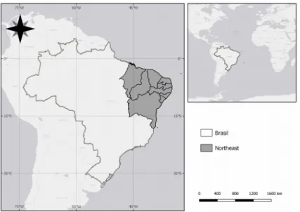
The study region is the Brazilian Northeast, commonly known as “Northeast”, which is an official political region of the country (Figure 1). The area of the region is approximately 1,56 million km² and the estimated population in 2018 was 56,76 million inhabitants [10]. The region is located between latitude 1° and 18° 30’ S and longitude 34° 20’ and 48° 30’ W and is constituted by nine states: Piauí, Ceará, Paraíba, Pernambuco, Alagoas, Sergipe, Maranhão, Rio Grande do Norte and Bahia. It stretches from the Atlantic seaboard in the northeast and southeast, northwest and west to the Amazon Basin and south through the Espinhaço highlands in southern Bahia. The Northeast is in a tropical zone and is characterized by diverse types of vegetation, such as Atlantic Forest and Caatinga, the latter being an ecosystem that thrives in a semi-arid region.
The Northeast region is characterized by high rates of illiteracy, low-income levels, migration to urban centers, social exclusion, among others. Besides cultural and economic differences, the region is affected by land degradation and desertification
exacerbated by anthropogenic factors. In climatic terms, the region is vulnerable to observed extremes of interannual climate variability, mainly droughts. In particular, the semi-arid region in the Northeast has been suffering from extremes of climate variability at various time scales, which have affected natural and social systems, especially people in socio-economic vulnerability conditions. Besides, climate change scenarios indicate that the region will be affected by rainfall deficit and increased aridity in the second half of 21st century [7].
Figure 1: Location of the study domain (Brazilian Northeast). METHODS AND DATA
We collected monthly data from 94 meteorological stations of the Brazilian National Meteorology Institute (INMET). The stations provide information about their latitude and longitude, elevation and average monthly temperature in Celsius degrees. Stations data from years 2000 to 2017 were selected for this study. The data are available online at the INMET website.
The data pre-processing consisted in transforming stations data into a more appropriate format for the analysis. Stations’ monthly average temperature were used to compute the average annual temperature. Since some stations had missing data for some months, a criterion of at least 9 months of data was used in order to compute the average annual temperature for each station. Hence, years that had less than 9 months of data have been left out of the analysis. After computing the average annual temperature for each station, the 2000-2017 timeframe was divided into two periods: Period 1 (2000-2008) and Period 2 (2009-2017). Then, based on the annual temperature, the average temperature was calculated for each of the stations and periods. The data were then exported to a shapefile format, with the spatial information being based on the stations’ latitude and longitude. Two datasets were created, one for each period. Hence, stations could be represented by points, having within their attribute table the value of average temperature for the corresponding period.
After the pre-processing, the analysis consisted in firstly performing an Exploratory Spatial Data Analysis (ESDA) of the average temperature for both periods. The ESDA
stage included calculating descriptive statistics, examining the spatial distribution using data posting, identifying clusters and outliers using the Local Moran’s I statistic, and testing the existence of a spatial autocorrelation pattern in the study domain based on the Global Moran’s I statistic. In a second stage, interpolated surfaces were produced using IDW and Ordinary Kriging. Afterwards, these interpolation methods were compared, as well as the surfaces from both periods, in order to evaluate possible changes in temperature patterns.
RESULTS
Descriptive statistics and exploratory spatial data analysis
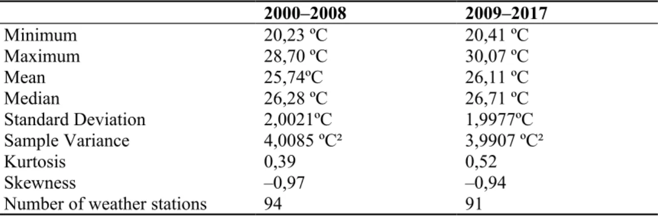
Descriptive statistics were computed to evaluate its behavior and check for inconsistencies (Table 1). There was an increase of 1,37ºC in the maximum, 0,18ºC in the minimum and 0,37ºC in the mean average temperature when comparing the two periods.
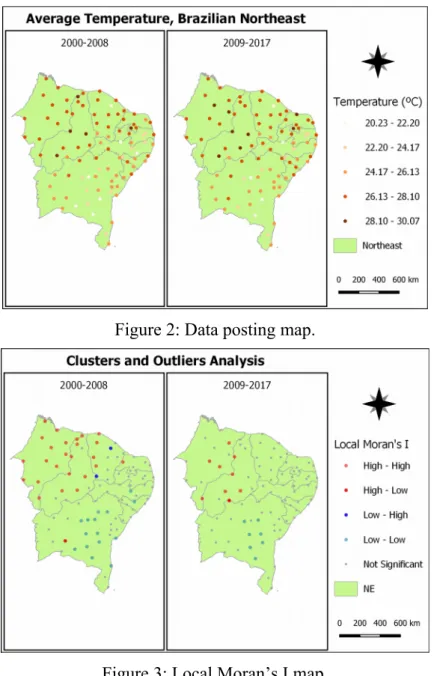
The data posting map (Figure 2) exhibits the distribution of the stations within the study region. It reveals that the lowest temperatures are concentrated in the southern part of the study region, whereas the highest appear to be in the center and in the north. Such pattern is fairly the same for both periods. The lower temperatures are concentrated mainly in the South of the study area, whilst the higher are located in the middle and in the north. In addition, there is an apparent trend in the data, since the temperature increases in the direction south-north, i.e. as it gets closer to the equator the temperature rises. However, there is no evidence of anisotropy, so for kriging interpolation purposes the attribute will be assumed isotropic.
Table 1: Descriptive statistics of the average temperature in weather stations.
2000–2008 2009–2017 Minimum 20,23 ºC 20,41 ºC Maximum 28,70 ºC 30,07 ºC Mean 25,74ºC 26,11 ºC Median 26,28 ºC 26,71 ºC Standard Deviation 2,0021ºC 1,9977ºC Sample Variance 4,0085 ºC² 3,9907 ºC² Kurtosis 0,39 0,52 Skewness –0,97 –0,94
Number of weather stations 94 91
The Local Moran’s I map (Figure 3) identifies spatial clusters and outliers. The results confirm that the lower values cluster in the south, and the higher in the center and north. The cluster pattern is similar for both periods analyzed. Furthermore, there is evidence of spatial outliers (i.e. high values correlate with low neighboring values, or vice versa). These are probably an expression of natural variation in the temperature within the region caused by the relief. The results of the Global Moran’s I statistics (Table 2) suggest that both 2000-2008 and 2009-2017 datasets exhibit (positive) spatial autocorrelation (given that the p-values are smaller than 0,01, the likelihood that the observed pattern could be the result of random chance is less than 1%).
Figure 2: Data posting map.
Figure 3: Local Moran’s I map. Table 2: Global Moran’s I statistics.
Moran’s Index Expected Index Variance z-score p-value
2000-2008 0,295 -0,011 0,0038 4,980 0,000001
2009-2017 0,248 -0,011 0,0037 4,281 0,000019
Difference in average temperature
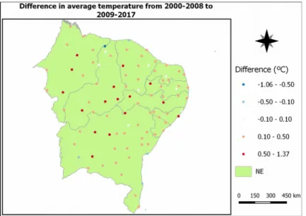
Figure 4 shows how the average temperature computed for each station varied between the two periods. Results indicate that 61 stations exhibited an increase of more than 0,1ºC, and 16 exhibited an increase of more than 0,5ºC. In addition, 9 stations had no significant change, i.e. the increase or decrease was lower than 0.1ºC, and only 5 stations featured a decrease greater than 0.1ºC. Therefore, there was an overall raise in the average temperature considering the periods of 2000-2008 and 2009-2017. In terms
of the intensity of the increase, the northwest, central and western regions seem to exhibit the most intense increase.
Figure 4: Difference in average temperature. Interpolated surfaces
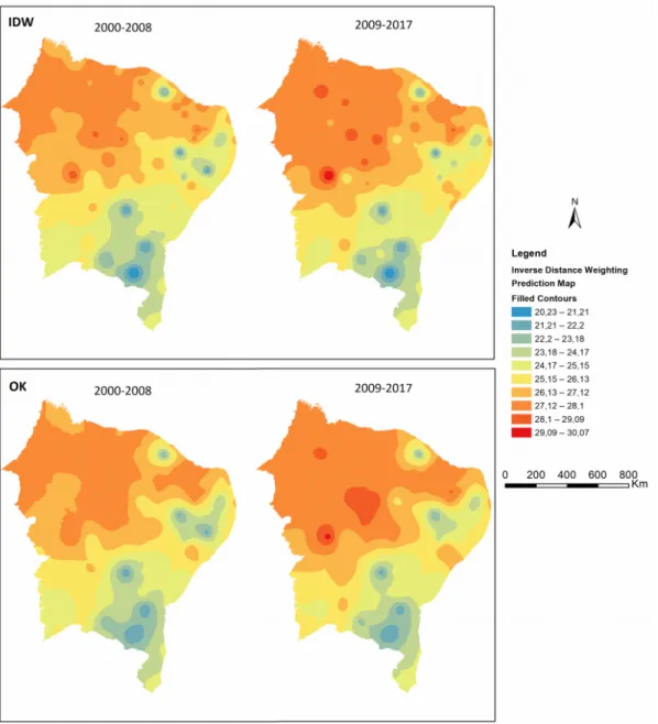
The data from the stations were used to produce interpolated surfaces of the average temperature in the study region. Figure 5 exhibits the predicted surfaces using the IDW method (top) and Ordinary Kriging (bottom). The semivariogram parameters used in kriging are detailed in Table 3, and the cross-validation error statistics are presented in Table 4.
Table 3: Semivariogram parameters.
2000-2008 2009-2017
Model Exponential Exponential
Nugget 0,35 0,35
Range (Km) 300 350
Total Sill 3,77 3,805
The methods have yielded reasonable results in terms of the error statistics. When comparing accuracy, IDW and kriging had similar values of the Root Mean Square Error. Regarding the biasedness of the predictions, kriging produced better results than the IDW (i.e., the Mean Errors were closer to zero). It is also noticeable that kriging generated smoother surfaces, reducing some of the bullseye aspect that IDW presented. Therefore, Ordinary Kriging performed better than IDW in both periods.
Table 4: Cross-validation error statistics.
IDW Ordinary Kriging
2000-2008 2009-2017 2000-2008 2009-2017
Mean Error -0,04569 -0,0416 -0,00789 -0,00653
In terms of change in the patterns of average temperature, the surfaces generated by both methods reveal that there was an overall increase in temperature. In the second period, the area representing the second warmest class (28,1 – 29,09ºC) spreads and covers areas that were previously cooler, especially in the north. Although changes are more noticeable in the north/northwest, the central and western regions of the study domain also exhibit an increase of temperature.
Figure 5: Interpolated surfaces of the average temperature. CONCLUSION
This work proposed to study temperature variability in the Northeast of Brazil. The analysis of the meteorological stations’ average temperature, in 2000-2008 and 2009-2017, revealed that the higher values are in the northern and central regions, whereas the lower values occur in the south and in the east. This pattern is identical for the two periods. However, observational data exhibit an overall increase of temperature values
within the whole study region, although in some areas the increase was more intense than in others. Furthermore, IDW and Ordinary Kriging methods were used to generate a continuous surface of the average temperature in each period. The Ordinary Kriging method produced better results than IDW in terms of unbiasedness of the predictions. Regarding the accuracy, the methods yielded similar results and it is not possible to affirm that one method was superior to the other based on this criterion. The temperature surfaces provide evidence of an increase in the extent of the area with higher temperatures in the 2009-2017 period, when compared with 2000-2008.
REFERENCES
[1] Cristóbal, J., Ninyerola, M., Pons, X., Modeling air temperature through a combination of remote sensing and GIS data, Journal of Geophysical Research:
Atmospheres, 113(D13106), 2008.
[2] Burrough, P. A., McDonnell, R. A., Principles of Geographical Information
Systems, Oxford University Press, 1998.
[3] Bhowmik, A. K., Costa, A. C., Representativeness impacts on accuracy and precision of climate spatial interpolation in data scarce regions, ‐ Meteorological Applications, vol. 22/issue 3, pp. 368-377, 2015.
[4] Martínez-Cob, A., Multivariate geostatistical analysis of evapotranspiration and precipitation in mountainous terrain, Journal of Hydrology, vol. 174/issue 1-2, pp 19-35, 1996.
[5] Goovaerts, P., Geostatistical approaches for incorporating elevation into the spatial interpolation of rainfall, Journal of Hydrology, vol. 228/issue 1-2, pp 113-129, 2000. [6] Haberlandt, U., Geostatistical interpolation of hourly precipitation from rain gauges and radar for a large-scale extreme rainfall event, Journal of Hydrology, vol. 332/issue 1-2, pp 144-157, 2007.
[7] Marengo, J., Alves Lincoln, M., Alyala, C. S., Cunha, A., Brito, S., Moraes, O., Climatic characteristics of the 2010-2016 drought in the semiarid Northeast Brazil region, Anais da Academia Brasileira de Ciências, vol. 90/issue 2, pp. 1973-1985, 2018.
[8] Selvaraju, R., Baas, S., Climate variability and change: adaptation to drought in
Bangladesh: A resource book and training guide, Italy, vol. 9, 2007.
[9] Marengo, J., Torres, R. R., Alves, L. M., Drought in Northeast Brazil – past, present and future, Theoretical and Applied Climatology, vol. 129/issue 3-4, pp. 1189-1200, 2017.
[10] Instituto Brasileiro de Geografia e Estatística, Estimativas da População Residente
no Brasil e Unidades da Federação, available online at ftp://ftp.ibge.gov.br/Estimativas_de_Populacao/Estimativas_2018/estimativa_dou_2018