Phylogenetic diversity of bird assemblages along different land-use gradients: regional and continental analysis

(1)

UNIVERSIDADE DE LISBOA

FACULDADE DE CIÊNCIAS

DEPARTAMENTO DE BIOLOGIA ANIMAL

Phylogenetic diversity of bird assemblages along different land-use

gradients: regional and continental analysis

Margarida Ladeira Felício Gonçalves

Dissertação

Mestrado em Biologia da Conservação

(2)

UNIVERSIDADE DE LISBOA

FACULDADE DE CIÊNCIAS

DEPARTAMENTO DE BIOLOGIA ANIMAL

Phylogenetic diversity of bird assemblages along different land-use

gradients: regional and continental analysis

Margarida Ladeira Felício Gonçalves

Dissertação orientada por Professor Dr. Roland Brandl, Departamento de

Ecologia,Phillips-Universität Marburg e Professor Dr. Carlos Fernandes, Departamento

de Biologia Animal, FCUL

Mestrado em Biologia da Conservação

(3)

Dedicatória

À minha mãe.

Embora ausente, o teu amor é a minha força, iluminando o meu caminho.

(4)

Thankful note/Agradecimentos

Primarily I would like to thank PhD Prof. Roland Brandl from Philipps-Universität Marburg for accepting me as his Master student, accompanying me and teaching me throughout my ERASMUS placement. For his patience, total availability, tolerance and dedication put upon my work.

To his workgroup, a special thanks to Eugene Egorov for all the patience, data and information provided and to Maike Franzen for all the co-work, company and friendship.

Um agradecimento ao Prof. Dr. Carlos Fernandes, da FCUL, por me ter aceitado como sua orientanda, pela disponibilidade e dedicação, sobretudo nos últimos meses de trabalho.

À sua equipa, queria agradecer pessoalmente ao André Silva pela disponibilidade e prontidão.

Ao meu Pai, pela força, esperança e amor. Por acreditar sempre em mim e no meu trabalho.

Aos meus irmãos, sobrinhos, cunhados e tios-avós pela força, apoio e preocupação.

(5)

Summary

Land-use intensification leads to the transformation of natural habitats into antrhopogenic ones, such as farmland and meadows or, in its widest sense, into urban areas. These habitats act as environmental filters, selecting only those species whose traits enables them to survive, and although a potential species richness increase, such species belong only to a set of a few lineages. Following an evolutionary conservative approach, it is thus expected a decrease of phylogenetic diversity of assemblages with increasing amount of transformed habitats.

The present study evaluates the phylogenetic diversity (mean phylogenetic and mean nearest neighbour distance) of native breeding bird assemblages, considering the impact of land-use at regional and continental scale, using Generalized Additive Models (GAMs); species richness was used for comparative reasons only. Regionally, across Bavaria, it was used presence/absence maps within 34 km2 grids and different land-use types; in a European-wide study it was analysed which factors contribute to this assemblage composition, in general and which of them differ between natural and antrhopogenic sites.

Overall it was found that the occurrence of bird species is driven by habitat filtering and not competition, regardless the scale of analysis. Within regional analysis although species richness increased with increasing percentage of anthropogenic land-use, both measures of phylogenetic diversity showed an overall decrease. For European-wide analysis, overall diversity was positivivelly related to area and climate. Natural and anthropogenic sites show

(7)

2 no significant differences, except only for species richness regarding body mass (g) and percentage of insectivores.

In a world where urbanization is increasing at an exponential rate it is important to analyse and recognize what processes and which factors contribute the most for shaping animal assemblages. These results confirm the elevated impact that anthropogenic habitats, especially urban areas, have upon shaping bird assemblages, acting as strong environmental filters, with a powerful evolutionary force.

Key-words: phylogenetic structure, habitat filtering, urbanization, Generalized

(8)

3

Resumo

A diversidade filogenética foi primariamente aplicada ao estudo da conservação, sendo que as espécies prioritárias eram seleccionadas com base na sua taxonomia. Hoje-em-dia, a importância da aplicação desta medida de biodiversidade extende-se também ao estudo das comunidades, promovendo o conhecimento dos processos evolutivos que levam à composição da sua estrutura filogenética, bem como da interacção existente entre as espécies constituintes. Dois processos são vistos como centrais nesta temática: (1) exclusão competitiva entre espécies que limita a sua coexistência a longo prazo; e (2) filtragem ambiental de espécies que persistem numa comunidade devido à sua tolerância a factores abióticos. O primeiro processo leva a uma sobre-dispersão filogenética, que tende a limitar a coexistência de espécies relacionadas entre si, conduzindo a uma diversidade filogenética superior à esperada sob condições aleatórias de estrutura comunitária. Pelo contrário, o segundo processo leva a um agrupamento filogenético, no qual espécies relacionadas tendem a coexistir e a diversidade filogenética revela-se menor que o esperado.

A intensificação do uso-da-terra tem, nas últimas décadas, levado à transformação do ambiente em habitats antropogénicos, nomeadamente em terrenos agrícolas e de pastoreio, ou num sentido mais extremo, em áreas urbanas. É do conhecimento geral que tais habitats altamente modificados actuam como filtros ambientais, selecionando apenas algumas espécies com determinadas características que lhes permitem sobreviver e que pertencem assim, a apenas deteterminadas linhagens. Seguindo um contexto evolutivo

(9)

4 conservacionista espera-se que, em áreas antropogénicas as espécies tendam a coexistir, levando à diminuição da diversidade filogenética, mesmo quando um aumento da riqueza específica se poderá também verificar.

Como tal, o presente estudo avalia a diversidade filogenética de comunidades de aves nativas nidificantes, considerando o impacte do uso-da-terra, tanto a nível regional como a nível continental. A diversidade filogenética foi calculada usando duas medidas diferentes: distância filogenética média, mais sensível a padrões que se verificam a nível geral, em toda a árvore; e a distância média ao vizinho mais próximo, mais sensível a padrões que ocorrem nas extremidades da árvore filogenética. Para a análise foram usados modelos estatísticos, nomeados Modelos Aditivos Generalizados (GAMs), nos quais a função de ligação dos Modelos Lineares é substituída por uma função não paramétrica, estimada através de curvas de alisamento que permitem descrever a forma da função e revelar possíveis não linearidades nas relações estudadas. A riqueza específica foi também incorporada, apenas para termos comparativos.

Regionalmente, o estudo foi efectuado no estado alemão da Baviera, usando dados de presença/ausência de espécies, recolhidos entre 1996 e 1999 em mapas com grelhas de cerca de 34 km2 e testando a influência da percentagem de diferentes tipos de uso-da-terra. A nível continental, foram usados estudos de presença/ausência documentados em vinte-e-dois países europeus entre 1973 e 2008, testando a influência da área de estudo e variação temporal na comunidade de aves europeias, bem como os diferentes factores que contribuem para a composição desta comunidade, em geral e os

(10)

5 que induzem a possíveis disparidades que se observam na composição entre a comunidade existente em ambientes naturais e a comunidade antropogénica.

Os resultados provenientes da distribuição espacial das espécies demostram que a ocorrência das espécies de aves analisadas é determinada por filtragem ambiental e não exclusão competitiva, independentemente da escala analisada. Isto leva a um processo de agrupamento filogenético e a uma menor diversidade filogenética do que seria de esperar sob condições neutrais. Na Baviera, como esperado, apesar de registado um aumento da riqueza específica com o aumento da percentagem de todos os tipos de uso-de-terra definidos, foi igualmente verificado um decréscimo da diversidade filogenética, para ambas as medidas calculadas. A nível europeu a riqueza específica e ambas as medidas de diversidade filogenética foram positivamente relacionadas com o aumento da área de estudo e clima, nomeadamente o aumento da temperatura. Contrariamente ao esperado, não foram detectadas diferenças significativas a nível filogenético entre ambientes naturais e antropogénicos; estas diferenças só ocorreram para a riqueza específica relativamente a duas variáveis: massa corporal (g) e percentagem de espécies insectívoras.

Estes resultados mostram, primariamente, a importância de incorporar não só diversas medidas de diversidade, bem como diferentes escalas de observação em estudos relativos à análise e gestão de comunidades. Mostram também o impacte que diferentes tipos de uso-da-terra, nomeadamente zonas urbanas, têm na organização e estruturação destas comunidades, actuando como ambientes filtradores que seleccionam as espécies com características que lhes permitem sobreviver e adaptar à presença constante do Homem. A

(11)

6 nível europeu, os resultados enfatizam a importância que áreas contínuas e de grande dimensão têm na gestão das comunidades de aves, sobretudo em zonas com condições climáticas favoráveis à reprodução e nidificação destas espécies, como por exemplo, em países do sul da Europa. Contrariamente ao esperado, não foram detectadas diferenças significativas entre comunidades europeias naturais e antropogénicas, no espaço temporal analisado; apenas foram detectadas diferenças em relação à riqueza específica, com maior número de espécies de menores dimensões e aumento do número de espécies com uma maior percentagem de aves insectívoras em zonas antropogénicas. A longo prazo, este processo selectivo poderá levar a um fenómeno de homogeneização biótica, intimamente ligado à perda de biodiversidade a nível global.

Este estudo promove, assim, a aplicação de acções de gestão que mantenham as espécies existentes e que aumentem a diversidade filogenética das comunidades analisadas, podendo os resultados ser abrangidos a outras regiões com características semelhantes, assim como a outros taxa existentes. Num futuro onde a urbanização crescerá a níveis exponenciais, é importante perceber as condições que estes habitats proporcionam e o potencial oferecido em termos de biodiversidade.

Palavras-chave: estrutura filogenética, filtragem ambiental, urbanização,

(12)

7

1. Introduction

1.1 Phylogenetic diversity and conservation

Understanding the mechanisms and processes that shape the distribution of phylogenetic diversity along environmental gradients can become crucial to the study of the potential effects of global change, identification of vulnerable ecosystems or species and the proposal of meaningful conservation measures to mitigate the current diversity crisis (Winter et al. 2013). Successful conservation strategies should thus retain as large an amount of phylogenetic diversity as available resources permit (Faith et al. 2004) and this parameter can be targeted directly into conservation planning (Rodrigues & Gaston 2002; Rolland et al. 2012).

Faith (1992) was among the first researcher that quantified phylogenetic diversity (PD) as the cumulative length of the branches connecting the root of the phylogenetic tree, representing the common ancestral lineage, to the evolving tips, represented by species. Phylogenetic branch lengths are a continuous metric of relatedness and this measure was primarily applied to conservation, where the priority taxa to be protected reflected a certain value of biodiversity (Minh et al. 2006). With the increasing availability of phylogenetic information it is now possible to develop more sophisticated methods to infer processes that structure the composition of species assemblages at different scales (Pavoine et al. 2005; Webb et al. 2002).

Conservation research has been primarily focused on a global-scale of phylogenetic diversity loss; however the loss of PD at smaller spatial scales is

(13)

8 of equal concern, since losing diversity at any scale can lead to a reduced potential for assemblages to respond to changing environmental conditions, through a reduction of genetic diversity (Morlon et al. 2011). Also, assemblages share a greater fraction of PD than species, suggesting that single isolated areas can be more efficient at preserving phylogenetic diversity than species richness (Swenson 2009).

1.2 Processes structuring assemblages

Species’ features are known to influence their interaction with other species and with the environment. If, on the one hand, phylogenetically closely related species are ecologically similar and therefore tend to co-occur, it is also expected that related species compete with each other, which constrains their coexistence (Losos 2008). In this way, depending on scale, bird assemblages are structured by a series of processes that can range from neutral or niche-based processes at small scales to speciation and global extinction at larger scales (Cavender-Bares et al. 2009). Such processes are expected to leave a distinct signal in the phylogenetic structure of assemblages (Cadotte et al. 2010) since ecologically similar species also tend to be phylogenetically related and therefore ecological factors of assembly composition are reflected in phylogenetic patterns (Helmus et al. 2007).

Niche-based processes may be divided into competitive interactions and environmental filtering. Assuming that phylogenetically related species occupy similar niches, competitive interactions should lead to assemblages in which species are phylogenetically less related (phylogenetic overdispersion) whereas

(14)

9 environmental filtering should lead to assemblages in which species are phylogenetically more related (phylogenetic clustering) when compared to assemblages solely structured by neutral processes (Burns & Strauss 2011; Emerson & Gillespie 2008; Kluge & Kessler 2011).

About 60 years ago researchers started to use the species to genus ratio as a simple measure of phylogenetic structure to search for competitive interactions, a niche-based process (Elton 1946). These competitive interactions should be particularly important between closely related species and therefore assemblages structured by competition should lead to a lower species to genus ration than expected by chance (Mayfield & Levine 2010).

The importance of the various processes that structure a community depends on spatial (and temporal) scale (Devictor et al. 2010). By previous studies (Vamosi et al. 2009) it is known that competitive interactions may become important on small scales whereas habitat filtering may be important on larger scales. Nevertheless, in a recent study (Gotelli et al. 2010) it has been shown for birds across Denmark, that competitive interactions leave a signal in the co-occurrence of species analysed on a grain size up to four orders of magnitude larger than the territory size, slightly contradicting previous statements.

1.3 Effect of anthropogenic land-use on phylogenetic diversity

Beside biotic processes, the most important determinant of specie’s distribution is the scattering of habitat across a landscape (Franklin 2009; Peres-Neto et al. 2012). Furthermore, the characteristics, distribution and area

(15)

10 of the various habitats are influenced by human activities, thereby changing the habitat that is available for the species across that landscape (Butler et al. 2010).

Anthropogenic land-use, defined as special human created habitats, such as farmland, meadows and urban areas, covers growing proportions of the global landscape (Filippi-Codaccioni et al. 2010). Particularly, agriculture and urbanization lead to fragmentation of natural areas, offering a set of special conditions for birds and other wildlife species by modifying processes like predation, interspecific competition and diseases, which structure bird assemblages. Only a subset of species may be able to cope with such special conditions (Alberti 2005). Consequently, one of the most recognized disturbances that may lead to niche-based processes in assemblages is human changed land-cover and land-use (Fuller & Gaston 2009). However, it is also known that anthropogenic habitats can accommodate an astonishingly rich flora and fauna, which can achieve large population sizes (Chiari et al. 2010; Hole et al. 2005; Rodewald & Shustack 2008).

1.3.1 Agriculture

Agriculture is considered the most important type of land use in Europe; however, nowadays it is also acknowledge that agricultural intensification is the major cause of decline in the abundance and diversity of bird species in this continent since the 1970’s (Donald et al. 2001). This intensification has led to the fragmentation and simplification of habitat, with increasing monocultures and fewer non-cultivated land, due to increased use of agrochemicals and

(16)

11 machinery, which reduces food and nest availability for birds (Batáry et al. 2007; Belfrage et al. 2005).

Nevertheless, a range of birds are still known to depend on agricultural land, especially in winter (Atkinson et al. 2005) and more than 50% of the existing habitats in Europe occur in farmland (Söderström et al. 2001), supporting more bird species of conservation concern than any other habitat type (Wilson et al. 2005). This is possible because throughout European countries one can find different farming systems and management practices [e.g. organic vs. conventional farming (Darnhofer et al. 2010; Fuller et al. 2005); set-aside land (Buskirk & Willi 2004); and agri-environment schemes (Donald & Evans 2006)], which result in a vast spectrum of specie’s responses (Reidsma et al. 2006).

1.3.2 Urbanization

Urbanization is a complex process of land conversion and it is now considered the fastest growing land-cover type, showing an exponential growth in Europe since the end of the 19th century (Antrop 2004). This process affects bird species through profound and permanent changes in the habitat (Bowman & Marzluff 2001).

However, much like agriculture, cities may also benefit birds through higher resource abundance, lower predator pressure (Jokimäki & Huhta 2000; Shochat et al. 2010), ameliorated climatic conditions, increased water availability and increased habitat availability that results from edge effects and ornamental vegetation (Marzluff 2005). Therefore, considered at the landscape

(17)

12 scale, cities may have a positive effect on species richness (Kühn et al. 2004; Mehr et al. 2011), especially due to an increasing adaptation from exotic species (Loss et al. 2009).

1.4 Aims

In a previous study, Pfeifer et al. (2009) evaluated bird species assemblages across Bavaria and discovered that species richness increased with increasing proportion of anthropogenic habitats, such as cities or industrial areas, when species richness was evaluated on a grain of approximately 34 km2. Similarly, a study on bats for the same area found also an increase of species richness with increasing percentage of anthropogenic habitats; however a decrease of phylogenetic relatedness between species (Riedinger et al. 2013). This leads to the idea that such modified habitats may have contrasting effects on species richness and phylogenetic diversity.

Following this, the main goal of the present study is to understand what phylogenetic signals anthropogenic habitats leave on native breeding bird assemblages, when focusing on different scales. At the regional scale across Bavaria on a grain of 34 km2 and by using broad habitat types, labelled

land-cover types; at the continental scale across Europe, along a spatial and

temporal gradient, using a grain from 1.04 and 108 333 km2 during thirty-five years, and also testing which factors contribute to significant differences between natural and anthropogenic assemblages.

More specifically it aims to 1) test the hypothesis that competitive interactions influence the distribution of native breeding bird species across

(18)

13 Bavaria, in particular and Europe, in general; 2) evaluate the phylogenetic structure of both assemblages, determining if they are more (phylogenetic clustering) or less related (phylogenetic overdispersion) than expected when compared with an assemblage structured by neutral processes; 3) test the hypothesis of an expected decrease of phylogenetic diversity with increasing proportion of anthropogenic habitats at regional scale; 4) evaluate wich factors contribute to the phylogenetic structure of European’s bird assemblage in general; and 5) test the hypothesis that natural and antrhopogenic areas within Europe present significant differences regarding some or all of these factors.

(19)

14

2. Methods

2.1 Data collection

Data collection was performed differently for both parts of the study, since they differ in the scale of analysis. Both regional and continental studies were thought considering the information available for bird community ranges and data resolution concerning land-use types, climate and ecological variables.

Regional analysis was performed in Bavaria, a federal state in the south east of Germany, covering an area of 70 547.82 km², half of which is classified as agricultural land. Annual mean temperature varies from 14.4 ˚C and 2.1 ˚C and mean annual precipitation between 850 mm and 1000 mm (Bezzel et al. 2005). Bird’s distribution originated from the same mapping project used by Pfeifer et al. (2009), using grid maps with information recorded between 1996 and 1999 collected by Bavaria’s Environmental State Secretary, Ornithology Station Garmisch-Partenkirchen (Bezzel et al. 2005). Each grid covered an average area of 33.9 km2 (minimum 32.9 km2; maximum 35.1 km2), and only grids fully within the Bavarian borders were used (1927 grid cells out of a total of 2285 – Appendix A). The presence/absence of native breeding bird species was recorded across these grids and only those who represented > 5% of total observations were used for the analysis, with the exception of those whose genera wasn’t represented yet, so that all genera recorded were present in the data (in total 157 species - Appendix B).

Continental analysis was achieved with a total of 127 studies reporting the presence/absence of bird species from 22 European countries collected

(20)

15 between 1973 and 2008 (Appendix C). Species were only selected if considered native and breeding within the country where they were present. Studies were categorized according to the level of human impact/urbanization of the site where they were performed: pristine sites to small fields, including several types of habitats (e.g. mountains, river sides and forests) were classified as Natural (80 studies); agricultural areas and villages with more than 1 000 inhabitants to capital cities were classified as Anthropogenic areas (47 studies). Species selection was the same as for Bavaria: only species with more than 5% of total observations were used for the analysis, with the exception of those whose genera wasn’t represented yet, so that all genera recorded were present in the data (in total 297 species - Appendix D).

2.2 Phylogeny

The basis for the evaluation of phylogenetic relatedness within assemblages was a phylogeny retrieved from a global phylogeny of birds (Jetz et al. 2012b). For both assemblages studied it was obtained a phylogeny corresponding to the species sampled in each matrix data, after the following process. First, for the species recorded in each assembalge a set with 100 phylogenies was retrieved from www.birstree.org using the Ericson All Species Source Tree [10 000 trees covering 9 993 species each (Jetz et al. 2012a)]. For each tree a distance matrix was calculated between species using the function

distTips in the add-on package adephylo in R (Jombart 2013) and after, the

mean distance across all 100 matrices. These matrices constitute an estimate of the phylogenetic distance between species and the distance was about twice

(21)

16 to the common ancestor. The final tree for each phylogeny (Appendix E & F) constituted the hierarchical cluster analysis of the previous calculated mean, using the un-weighted average linkage algorithm.

2.3 Spatial distribution of species

In order to test the hypothesis that competitive interactions influence the distribution of species for both assemblages, it was used the function

comm.phylo.cor in the add-on package picante in R (Kembel 2010) with 999

randomizations to evaluate significance. This function characterizes the distributional overlap across a community, checking for a correlation between co-occurrence patterns of species and phylogenetic distance between them.

This index is based upon Schoener’s index, originally used to measure overlap in habitat use or diet (Schoener 1970). An index of 0 indicates that two species never occur together in the same grid and an index of 1 indicates that the two species always occur together. Other available indexes were used (Jaccard, Checkerboard and DOij indexes), since they only differ by the way co-occurrence is estimated and therefore provide almost the same results (Hardy 2008).

2.4 Phylogenetic structure of assemblages

After this, and also using the add-on package picante in R, it was evaluated the phylogenetic structure of the assemblages, using the matrix of average phylogenetic distance and by calculating the standardized effect size of

(22)

17 the mean phylogenetic distance (SESMPD) and of the mean nearest neighbour

distance (SESMNTD), whose functions are as follows:

( )

where index.obs is, respectively, the observed mean phylogenetic distance or mean nearest neighbour distance in communities; index.rand.mean is the mean distance calculated from a null model and index.rand.st is the standard deviation of the index across null communities. Values < 0 indicate phylogenetic under-dispersion (clustering) whereas values > 0 indicate phylogenetic over-dispersion. The null model was obtained by reshuffling species names across the tips of the phylogeny, using 999 runs. This model keeps the occurrence, as well as recorded number of species within grids unchanged.

2.5 Effects of anthropogenic land-use on phylogenetic diversity

2.5.1 Definition of land-use, bioclimatic and trait variables

To test for the hypothesis of a decrease phylogenetic diversity with increasing proportion of anthropogenic land-use types at regional scale and evaluate the factors that contribute to European assemblage as well as for differences between natural and antrhopogenic sites, it was analysed the response of the effect size of the mean phylogenetic distance as well as the effect size of the mean nearest neighbour distance to different land-use variables and both area and time variation. It was also analysed the response of

(23)

18 space (Latitude and Longitude), bioclimatic and trait variables as control. This process was achieved using Generalized Additive Models – GAMs.

For Bavaria, it was used the same land-use (habitat) and climate data as both Pfeifer et al. (2009) and Riedinger et al. (2013). Data included one set that characterized the climate, extracted from the 19 bioclimatic variables available in WorldClim (http://www.worldclim.org) using a spatial resolution of 30 seconds. The second set of data consisted of percentages of area covered by broad habitat types in each grid and its location (Latitude and Longitude). This land-cover was derived from the land-cover classes after the European wide mapping project CORINE (Coordinated Information of the European Environment), which uses LANDSAT-7 satellite images (scale 1:100 000) collected in 2000 (http://www.corine.dfd.dlr.de). Several classes were grouped into seven broad land-use types (Table 1), which were used in subsequent analysis. Both data sets were read into ArcGis 10.2.

For continental analysis each study was characterized by both a spatial compoent, representing the dimension of the study-area in km2, with a minimum area of 1.04 km2 and a maximum area of 108 333 km2 and a temporal component, represented by the average year of each study, along thirty-five years. Land-use was performed by quantatively selecting the study-site as natural or anthropogenic, as mentioned earlier and climate was analysed using only 4 of the 19 bioclimatic variables from WordClim, since only these were thought to best define the seasonality differences that occur intra-continent (bio5, bio6, bio13 and bio14). Climate data was also read into ArcGis 10.2.

(24)

19

Table 1. Land-use types formed from the CORINE land-cover classes. For each class it was

given the code used by the CORINE web site.

Land-use types Code CORINE land-cover classes

Farmland

211 Non-irrigated arable land

221 Vineyards

222 Fruit trees and berry plantations

Meadow

231 Pastures

243 Agricultural land with areas of natural vegetation

321 Natural grassland

Wetland

322 Moors and heathland

411 Inland marshes

412 Peat bogs

331 Beaches, dunes, sand

511 Water courses

512 Water bodies

Deciduous forest 311 Broadleaf forest

Coniferous forest 312 Coniferous forest

Mix forest 313 Mix forest

Anthropogenic habitats

121 Industrial, commercial and public units

124 Airport

131 Mineral extraction sites

132 Dump sites

111 Continuous urban fabric 112 Discontinuous urban fabric

123 Port areas

133 Construction sites

141 Green urban areas

142 Sport and leisure facilities

122 Road and rail networks and associated land

For both assemblages it was also added a trait set characterizing biological variables for each species analysed, including body mass (g), trophic niche, clutch size (Cramp et al. 1994; Dunning 1993) and population size

(25)

20 (retrieved from http://www.iucnredlist.org and http://birdlife.org) since all of them contribute for specie’s sensitivity to human impact and consequent priority for management planning. All of these variables, although specie’s specific were converted into assembalge based, in order to minimize within site/study variation due to specie’s trait differences. This was accomplished by calculating the logarithmic mean of body mass (g), clutch size (per year) and population size (pairs x 10000), averaged across all species that were present on each site or study and average percentage of species with each diet category (e.g. carnivores) (Table 2 & 3).

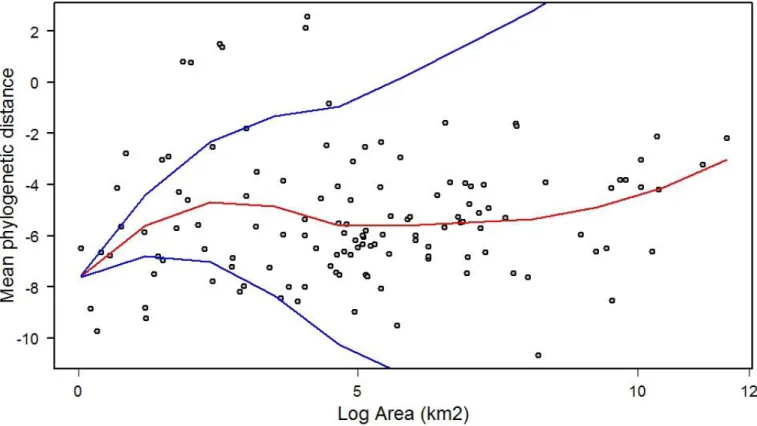
Table 2. Trait variables analyse for Bavarian assemblage. SD stands for standard deviation;

also included the 25% and 97.5% range of each trait sample.

Bavaria Mean ± SD 25% 97.5% Body mass (g) 48.36 ± 9.446 42.439 67.046 % Carnivores 9.890 ± 2.899 7.828 15.058 % Insectivores 44.46 ± 3.629 42.169 51.341 % Omnivores 27.17 ± 3.223 25 34.311 % Piscivores 1.583 ± 1.380 0 4.440 % Granivores 16.890 ± 2.605 15.068 22.346 % Scavengers 0.295 ± 0.605 0 1.754

Clutch size (year) 5.980 ± 0.228 5.835 6.456

(26)

21

Table 3. Trait variables analyse for natural and anthropogenic sites within European-wide

assemblage. SD stands for standard deviation; also included the 25% and 97.5% range of each trait sample.

Since the bioclimatic set contained a large amount of data and variables were highly correlated, this set was summarized with principal component analysis based on the correlation matrix for each assemblage and then the first two principal components where used for further analysis (Appendix G). Both components summarized together an average of 70% of the total variance. In a general way, PC1 is a measure of annual temperature and precipitation whereas PC2 measures the seasonal variability of the climate.

Before anyfurther analysis it is important to test the existence of collinearity between response variables in order to prevent weak results and facilitate variables’ relation prediction (Dormann et al. 2013). Collinearity was tested with simple pairwise correlation coefficient (r) for each variable within each assemblage and the threshold was set at r > 0.7.

European natural sites European anthropogenic sites

Mean ± SD 25% 97.5% Mean ± SD 25% 97.5% Body mass (g) 73.99 ± 42.078 52.374 163.589 50.28 ± 13.070 41.761 75.041 % Carnivores 10.5 ± 4.060 8.649 18.193 8.575 ± 2.881 5.742 12.617 % Insectivores 49.17 ± 4.848 45.213 60.031 47.13 ± 4.933 43.584 52.549 % Omnivores 23.98 ± 4.132 20.572 31.119 26.25 ± 4.361 23.181 35.635 % Piscivores 3.143 ± 2.890 1.127 12.071 1.579 ± 1.364 0 4.85 % Granivores 13.880 ± 3.704 11.746 21.966 15.840 ± 3.967 12.596 22.228 % Scavengers 0.710 ± 0.760 0 2.592 0.189 ± 0.350 0 0.959

Clutch size (year) 5.633 ± 0.415 5.384 6.333 5.830 ± 0.252 5.652 6.256

Population size (pairs

(27)

22 For both Bavarian and European assemblages it was found a high correlation between Latitude and PC1 (Bavarian r = 0.71; Anthropogenic sites r = 0.85; P < 0.001) and clutch size and population size (Bavarian r = 0.77; Anthropogenic sites r = 0.99; P < 0.001), so both Latitude and clutch size were removed from both data. Only for Europe, the percentage of Piscivores and body mass were highly related (r = 0.75; P < 0.001), so the first variable was removed from this data.

2.5.2 Generalized Additive Models

Generalized Additive Models – GAMs – were first introduced by Hastie & Tibshirani (1986) and are extensions of Generalized Linear Models (GLMs) where the linear predictor is given by a specified sum of smooth functions of covariates. It can be simply defined as follows:

( ) ( ) ( )

where the response variable

y

i can be defined by smooth functions k1 and k2 of covariates

x

1 and

x

2. It predicts some known smooth monotonic function of the expected value of the response variable, which may follow any exponential family distribution, permitting the use of a quasi-likelihood approach (Wood 2006).

The effect sizes of the mean phylogenetic distance and of the mean nearest neighbour distance were used as response variables for statistical analysis using function gam from package mgcv in R (Wood 2013). For

(28)

23 comparative reasons it is also used the value of species richness. This package solves the smoothing parameter estimation problem using the Generalized Cross Validation (GSV) criterion, based upon the number of data, deviance and effective degrees of freedom of the implemented model. The lower the GSV score the better the model, with higher percentage of deviance explained.

For Bavaria, land-use data, both principal components of the climate data and trait data were used as independent variables; for European-wide assemblage it was the same, except for the land-use data analysis, which was characterized by a factor that indicated if a study belonged to the natural or

antrhopogenic data set and the addition of both spatial and temporal

components within each site. This method of Generalized Additive Models allows fitting curvilinear relationships and for this analysis it was used thin plate splines as smoothers, starting with the default settings (k = 10) for Bavaria and decreasing it to 5 for European-wide assemblage to obtain more robust models, since the number of replicates was lower. Also, for European analysis the land-use factor was added to the model in two different ways: individually, without a smooth function describing it; and as a by-function for each independent variable, allowing testing for significant differences between data-sets, within Europe.

Furthermore, trait data can sometimes present a high correlation with phylogenetic measures and space data always shows spatial autocorrelation, which compromises additionally hypothesis testing. To remove the first correlation, it was increased the default of the dimension of the basis used to represent the smooth terms for trait variables and to control for spatial autocorrelation it was also included the factor space in the gam models [see

(29)

24 also Dormann et al. (2007)]. For Bavaria the default of the dimension used to represent the smooth term was increased to 40 and for European assemblage to 10.

Also, the available significance tests for the smoothers are only aproximate, and so it was followed a conservative approach, accepting significance only if P < 0.01.

(30)

25

3. Results

3.1 Spatial distribution of species

The correlation between the phylogenetic distance averaged across all 100 distance matrices of the bird species with their co-occurrence was significantly negative for both assemblages (Bavaria matrix correlation = - 0.29; European matrix correlation = - 0.22; P ≈ 0.001). This means that phylogenetic related species tend to co-occur more than expected, regardless the scale of analysis.

Calculating this matrix correlation using distance matrices of each of the 100 trees retrieved for each assemblage analysed, also showed a negative correlation for all matrices, with similar average numbers (Figure 1).

Figure 1. Histograms showing the distribution of matrix correlations for all 100 trees for both Bavarian

(31)

26

3.2 Phylogenetic structure of assemblages

The effect size of the mean phylogenetic distance and of the mean nearest neighbour distance were moderately correlated for Bavaria and European-wide assemblages (Bavarian r = 0.19; P < 0.001; European-wide r = 0.28; P < 0.01; both not corrected for spatial autocorrelation). The effect size of the mean phylogenetic distance also showed a moderate to low correlation with species richness for both assemblages (Bavarian r = 0.12; P < 0.001; European r = 0.18; P < 0.05; both not corrected for spatial autocorrelation).

Averaged across all grids and studies, the effect sizes of the mean phylogenetic distance as well as of the mean nearest neighbour distance were negative for both assembalges and differed significantly from zero (Bavarian SESMPD = - 4.37; t = -138.7; P < 0.01; Bavarian SESMNTD = -1.24; t = - 42; P <

0.001; European SESMPD = - 5.31; t = - 24.2; P < 0.001; European SESMNTD = -

1.88; t = - 19.6; P < 0.001), indicating community clustering in respect to phylogeny at both tree-wide and closer-to-tips phylogenetic scale, regardless of scale.

3.3 Effects of anthropogenic land-use on phylogenetic diversity

Considering Bavaria, GAMs results showed a relationship between land-use variables and both measures of phylogenetic diversity, as well as species richness (Table 4). The effect size of the mean phylogenetic distance was related to meadows and anthropogenic habitats, presenting a decrease with the increasing percentage of both (Figure 2).

(32)

27

Table 4. Results from Generalized Additive Models performed for Bavarian assemblage using species richness and both measures of phylogenetic

diversity as response variables. Est. Std. represents the estimated standard deviation; Std. Error the estimated error. Edf represents the estimated degrees of freedom for each independent variable; Ref. df the estimated residual degrees of freedom for each variable. For each response variable is also presented the R-square adjusted value - R-sq (adj) –, the GSV score and the explained deviation of each model. Significant values (P < 0.01) are highlighted. For the land-use types, highlighted F values show an increase of the response variable with that land-use type variable.

Species richness Mean phylogenetic distance Mean nearest neighbour distance

Est. Std. Std. Error t-value P Est. Std. Std. Error t-value P Est. Std. Std. Error t-value P Intercept 72.315 0.199 361.700 < 0.001 -4.368 0.012 -362.900 < 0.001 -1.241 0.017 -74.200 < 0.001

Edf Ref. df F P Edf Ref. df F P Edf Ref. df F P

PC1 climate 3.378 4.287 15.260 < 0.001 1.000 1.000 2.681 0.102 1.000 1.000 20.227 < 0.001

PC2 climate 5.453 6.610 9.014 < 0.001 3.492 4.442 4.404 < 0.001 1.000 1.000 0.266 < 0.01

Space 22.755 27.640 3.473 < 0.001 8.919 11.156 20.976 < 0.001 2.374 3.039 3.765 0.010

Farmland 1.473 1.810 21.270 < 0.001 4.044 5.013 1.566 0.166 1.000 1.000 0.112

(33)

28

Species richness Mean nearest neighbour distance Mean phylogenetic distance

Meadow 1.000 1.000 44.479 < 0.001 3.880 4.834 8.384 < 0.001 3.438 4.313 2.891 0.020 Wetland 4.351 5.283 8.388 < 0.001 1.000 1.000 0.740 0.390 1.960 2.469 7.823 < 0.001 Coniferous forest 3.021 3.817 6.204 < 0.001 3.183 4.017 5.058 < 0.001 4.449 5.500 1.008 0.412 Deciduos forest 1.588 1.972 6.447 < 0.001 1.012 1.024 2.802 0.093 2.120 2.659 3.099 0.032 Mix forest 1.000 1.000 4.364 0.037 1.000 1.000 23.676 < 0.001 2.982 3.737 1.989 < 0.001 Anthropogenic habitats 1.077 1.150 89.362 < 0.001 1.000 1.000 39.900 < 0.001 4.126 5.124 4.338 < 0.001 Body mass 4.708 5.919 22.361 < 0.001 5.109 6.377 480.892 < 0.001 5.305 6.609 1.258 0.268 Pop. size 14.380 17.330 5.587 < 0.001 12.843 15.555 4.342 < 0.001 2.558 3.099 34.201 < 0.001 Carnivores 9.303 11.605 5.642 < 0.001 35.842 37.525 3.839 < 0.001 12.807 15.841 1.928 0.015 Insectivores 4.679 5.995 16.566 < 0.001 12.366 15.202 4.755 < 0.001 1.000 1.000 6.166 0.013 Omnivores 14.982 18.459 6.633 < 0.001 5.587 7.122 7.071 < 0.001 7.566 9.527 3.198 < 0.001 Piscivores 20.512 24.551 7.954 < 0.001 8.176 10.008 4.380 < 0.001 1.000 1.000 63.091 < 0.001

(34)

29

Species richness Mean nearest neighbour distance Mean phylogenetic distance

Granivores 12.376 15.215 5.236 < 0.001 10.348 12.801 2.481 < 0.01 2.565 3.481 1.438 0.222

Scavengers 8.715 10.566 21.144 < 0.001 3.795 4.630 25.324 < 0.001 3.344 4.054 5.698 < 0.001

R-sq (adj.) 0.724 0.854 0.228

GSV score 82.872 0.298 0.557

(35)

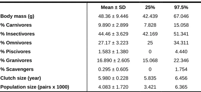
30 The effect size of the mean nearest neighbour distance was related to wetlands and anthropogenic habitats. It showed a moderate decrease with the increasing percentage of the first and with the second presented a hump-Figure 2. Scatterplots of the Generalized Additive Model for Bavarian assemblage relative to the

effect size of mean phylogenetic distance versus percentage of anthropogenic habitats (on top) and percentage of meadows (on bottom). Red line represents the fit evaluated at the mean of the independent variable and blue lines represent the fitted lines of ± two times the standard error of the independent variable.

(36)

31 shaped relationship, where nearest neighbour distance increased slightly until the percentage of anthropogenic habitats reached about 15% and beyond this point it decreased (Figure 3).

Figure 3. Scatterplots of the Generalized Additive Model for Bavarian assemblage relative

to the effect size of mean nearest neighbour distance versus percentage of wetlands (on top) and percentage of anthropogenic habitats (on bottom). Red line represents the fit evaluated at the mean of the independent variable and blue lines represent the fitted lines of ± two times the standard error of the independent variable.

(37)

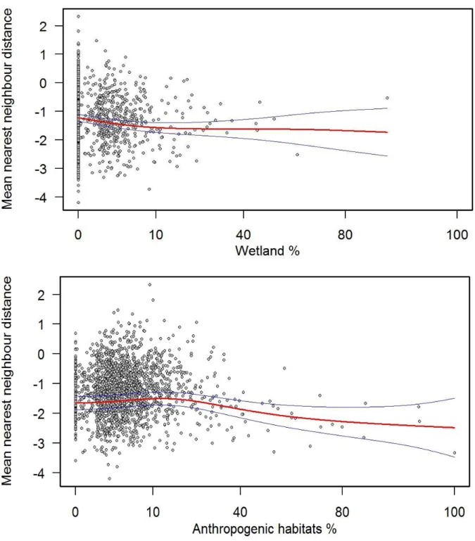
32 Species richness increased with the increased percentage of wetlands, meadows (Figure 4), farmland and anthropogenic habitats (Figure 5).

Figure 4. Scatterplots of the Generalized Additive Model for Bavarian assemblage relative to

species richness versus percentage of wetlands (on top) and percentage of meadows (on bottom). Red line represents the fit evaluated at the mean of the independent variable and blue lines represent the fitted lines of ± two times the standard error of the independent variable.

(38)

33 Influence of climate variables and of total or single trait variables were always significant for all three response variables (Table 4).

Figure 5. Scatterplots of the Generalized Additive Model for Bavarian assemblage relative to

species richness versus percentage of farmland (on top) and percentage of anthropogenic habitats (on bottom). Red line represents the fit evaluated at the mean of the independent variable and blue lines represent the fitted lines of ± two times the standard error of the independent variable.

(39)

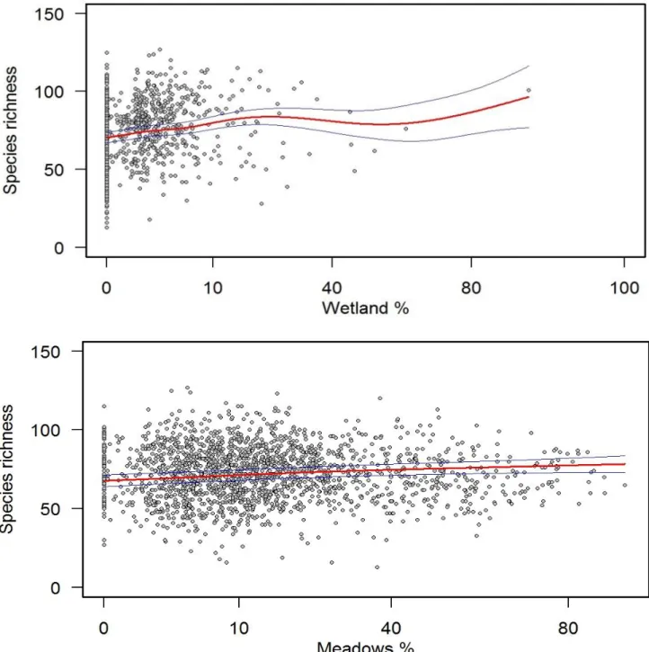
34 Considering European-wide assemblage, Generalized Additive Models results presented significant relationship between the spatial component and the effect size of the mean phylogenetic distance, as well as with species richness (Table 5), with increased phylogenetic diversity (Figure 6) and number of species (Figure 7) with area (km2).

Climate was significantly related to all three response variables, with increasing species richness and overall phylogenetic diversity with increasing mean annual temperature and low precipitation (PC1). Space had no influence in any of the variables; total or single trait variables were always significant for all three response variables.

Figure 6. Scatterplot of the Generalized Additive Model for European-wide assemblage relative to the

effect size of mean phylogenetic distance versus area (log in km2). Red line represents the fit evaluated at the mean of the independent variable and blue lines represent the fitted lines of ± two times the standard error of the independent variable.

(40)

35

Table 5. Results from Generalized Additive Models performed for European-wide assemblage using species richness and both measures of

phylogenetic diversity as response variables. Est. Std. represents the estimated standard deviation; Std. Error the estimated error. Edf represents the estimated degrees of freedom for each independent variable; Ref. df the estimated residual degrees of freedom for each variable. For each response variable is also presented the R-square adjusted value - R-sq (adj) –, the GSV score and the explained deviation of each model. Significant values (P < 0.01) are highlighted. Regarding the independent variables, highlighted F values show an increase of the response variable with that independent variable. It is also showen the results of the land-use factor interaction with each independent variable, allowing a between natural and anthropogenic sites interpretation.

Est. Std. Std. Error t value |t| Est. Std. Std. Error t value |t| Est. Std. Std. Error t value |t| Intercept 123.785 5.257 23.546 < 0.001 -5.434 0.268 -20.270 < 0.001 -1.554 0.307 -5.065 < 0.001 Land-use 13.371 9.630 1.389 0.170 -0.371 0.404 -0.920 0.360 0.207 1.743 0.119 0.906

PC1 climate 3.626 3.879 9.450 < 0.001 3.307 3.705 4.032 < 0.01 1.000 1.000 13.468 < 0.001

(41)

36

Space 2.566 3.181 2.305 0.081 2.682 3.340 1.019 0.390 1.893 2.360 1.534 0.214 Area 3.791 3.954 27.377 < 0.001 1.000 1.000 11.895 < 0.001 1.000 1.000 0.000 0.987 Year 2.123 2.580 1.641 0.190 2.723 3.243 3.228 0.024 1.000 1.000 0.022 0.884 Body mass 3.801 3.955 5.689 < 0.001 2.897 3.415 13.967 < 0.001 2.021 2.527 3.934 0.016 Pop. size 2.584 3.069 8.390 < 0.001 1.000 1.000 0.017 0.896 3.972 3.997 2.653 0.039 Carnivores 2.640 3.201 2.898 0.038 1.000 1.000 5.524 0.021 3.518 3.876 8.167 < 0.001 Insectivores 3.148 3.553 3.466 0.016 1.847 2.249 3.268 0.038 2.027 2.470 2.113 0.115 Omnivores 3.936 3.990 8.461 < 0.001 2.503 3.004 1.626 0.189 1.000 1.000 10.444 < 0.01 Granivores 2.927 3.361 4.707 < 0.01 3.527 3.782 4.148 < 0.01 1.000 1.000 9.560 < 0.01 Scavengers 3.836 3.961 5.843 < 0.001 3.506 3.825 6.844 < 0.001 2.368 2.809 2.756 0.051 Land-use*PC1 climate 1.073 1.073 1.893 0.170 1.077 1.077 0.396 0.546 1.077 1.077 0.006 0.947

(42)

37

Land-use*PC2 climate 2.098 2.513 0.626 0.573 1.077 1.077 1.728 0.189 1.077 1.077 0.181 0.691 Land-use*Space 2.561 2.974 3.555 0.019 1.422 1.650 1.955 0.149 2.461 2.905 0.969 0.406 Land-use*Area 1.073 1.073 1.829 0.178 1.077 1.077 1.468 0.227 2.275 2.631 2.794 0.052 Land-use*Year 2.164 2.620 1.749 0.168 1.077 1.077 0.761 0.389 1.077 1.077 0.191 0.682 Land-use*Body mass 2.881 3.051 6.926 < 0.001 1.077 1.077 0.064 0.819 1.077 1.077 0.122 0.747 Land-use*Pop. size 1.073 1.073 1.062 0.306 1.077 1.077 0.930 0.339 1.077 1.077 1.371 0.243 Land-use*Carnivores 1.073 1.073 4.491 0.035 1.077 1.077 2.729 0.099 1.077 1.077 0.455 0.516 Land-use*Insectivores 3.971 4.047 7.788 < 0.001 2.854 3.304 0.906 0.446 2.701 3.171 1.853 0.140 Land-use*Omnivores 1.073 1.073 0.936 0.338 1.077 1.077 2.137 0.144 1.077 1.077 0.305 0.560 Land-use*Granivores 1.917 2.293 2.353 0.095 2.732 3.234 1.014 0.392 3.724 3.978 2.916 0.026 Land-use*Scavengers 1.073 1.073 1.761 0.186 1.077 1.077 1.938 0.164 2.010 2.116 0.491 0.624

(43)

38

R-sq (adj.) 0.964 0.898 0.704

GSV score 124.560 0.963 0.527

(44)

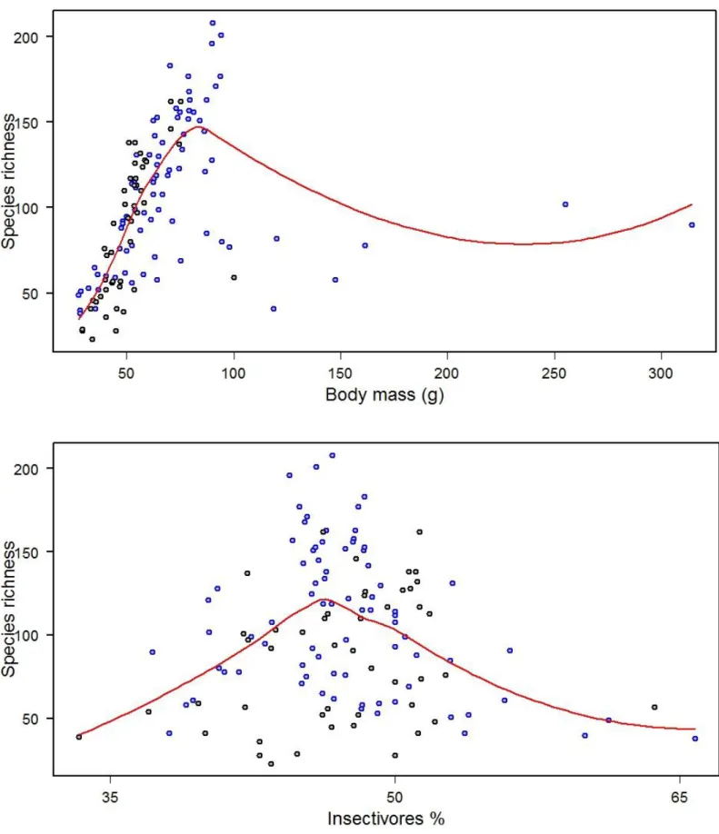
39 Relative to the effect of the land-use factor, it was only significant for species richness regarding species’ body mass (g) and percentage of Insectivores, indicating significant differences between natural and antrhopogenic sets for both variables (Table 5). Studies composed of bird species with average body mass between 50 and 100 g are those who contribute more to species richness at European-wide scale. It’s in natural sites where this variable reaches its highest value and also where it can be found the sites with the biggest animals (Figure 8). Considering the percentage of insectivorous species, it presents an assymptotic relationship with species richness, with higest richness in natural sites where there are about 40% insectivores and in anthropogeic sites where there are about 55% insectivores, assemblage wide. It’s also in natural sites where it can be found the highest percentage of insectivores (Figure 8).

Figure 7. Scatterplot of the Generalized Additive Model for European-wide assemblage relative to

species richness versus area (log in km2). Red line represents the fit evaluated at the mean of the independent variable and blue lines represent the fitted lines of ± two times the standard error of the independent variable.

(45)

40

Figure 8. Scatterplots of the Generalized Additive Model for European-wide assemblage relative to species

richness versus body mass (g) (on top) and percentage of insectivores (on bottom), with significant differences considering land-use. Red line represents the fit evaluated at the mean of both independent variables. Blue dots represent natural sites; black dots represent antrhopogenic sites.

(46)

41

4. Discussion

4.1 Spatial distribution and phylogenetic structure of assemblages

Assemblage-wide analysis of co-occurrence as well as overall patterns of phylogenetic relatedness within assemblages measured by the mean phylogenetic distance as well as by the mean nearest neighbour distance showed that, regardless of considered grain, environmental filtering is more important than competitive interactions in shaping bird assemblages.

This is similar to the results obtain for bats within Bavaria (Riedinger et al. 2013) but contradicts the findings from Denmark (Gotelli et al. 2010), which showed signs of competition across a similar spatial scale. Like Denmark, present-day Bavaria offers an ideal geographic setting for co-occurrence analysis of avian species at regional scale, since there are no major geographic barriers to avian dispersal. Furthermore, no in situ speciation occurred in Bavaria, otherwise endemic species or at least subspecies should occur. However, Gotelii et al. (2010) analysed the structure within selected guilds whereas the present study used all genera observed. Therefore, the present approach might have diluted signs of competition.

However, using the approach followed on the present study it is possible to conclude that across all genera which may occur on a grid, competition is in general not important, given the assumption that the intensity of competitive interactions decreases with increasing phylogenetic intensity. Therefore, the present analysis is not showing that competition is not occurring; it states only that it is not important for the distribution of species at the considered grain.

(47)

42 Although it might seem contradictory that similar species can be able to co-exist and competitive interactions might be overcame, in other studies (Stamps 1991; Stephens & Sutherland 1999) it has been acknowledge that a positive relationship between the suitability of a patch and the number of conspecifics is not uncommon, leading to aggregative behaviour, even in territorial birds. This, allied with the fact that sometimes bird species can aggregate to form colonies during breeding season, might contribute to clustering of the assemblages studied and the co-occurrence found.

4.2 Anthropogenic land-use impact

At the regional level, for Bavaria, and according to previous predictions, there was an overall decrease of both measures of phylogenetic diversity with increased percentage of land-use, more specifically, anthropogenic habitats and meadows. This decrease occurred despite the fact that species richness was significantly increasing with the percentage of most land-type analysed, even when only native species were selected.

Both measures of phylogenetic diversity capture a different aspect of the phylogenetic structure. Mean phylogenetic distance is thought to be more sensitive to tree-wide patterns of phylogenetic clustering and evenness (Kembel 2010). Mean nearest neighbour distance, which is the mean distance that separates each species in the community from its closest relative, is thought to be more sensitive to patterns close to the tips of the phylogeny (Kraft et al. 2007).

This difference is already evident when comparing the distribution of effect sizes between both measures, since, although both were negative, the

(48)

43 effect size of the mean phylogenetic distance was always more negative than the effect size of the mean nearest neighbour distance.

Considering bird’s evolutionary history, Aves class is divided into Paleognathae (compromising ratites and tinamous) and Neognathae (all others); furthermore, the last one is split into Galloanserae (chickens, ducks and allies) and Neoaves (all others) (Hackett et al. 2008).

The slight, punctual increase of the effect size of mean nearest neighbour distance with the percentage of anthropogenic habitats (until 15% of their occupancy) can be explained by the occurrence of numerous species of birds belonging to the lineage of the Galloanseres. Increasing percentage of existing water within city parks and gardens within anthropogenic habitats leads to momentary increase of these species, highly associated with water availability and/or open habitats.

Furthermore, this lineage diverged from the Neoaves in the Mid-Cretaceous (120 to 90 M.y. ago). When analysing the effect size of the mean phylogenetic distance all pairs of species belonging to both lineages are included and therefore the influenced of Galloanseres presence is deluded, leading to decreasing values. In contrast, the effect size of the mean nearest neighbour distance includes only pairs within each lineage and its value becomes higer. This suggests that habitat affiliation evolved very early in the history of birds [e.g. Prinzing et al. (2001) for plants].

In agreement with other studies from plants in Germany (Knapp et al. 2008) and bats in Bavaria (Riedinger et al. 2013) in the present study and in particular for anthropogenic habitats, although species richness increased, phylogenetic diversity decreased with the percentage of such land-type. This

(49)

44 means that, also for birds, the necessary traits to cope with the pressures of urban habitats are confined to certain lineages, less sensitive to human presence. It may indicate that with the further increase of species with increasing amount of urban habitats, species from already occurring lineages are added to the assemblages, a clear sign of habitat filtering.

Overall, the hump-shaped relationship found between the effect size of the mean nearest neighbour distance and anthropogenic habitats can be explained by the intermediate disturbance hypothesis (Wilkinson 1999). A small level of urbanization within an area can lead to more complex and heterogeneous conditions, supporting more species of birds, and consequently, more different lineages, especially in suburban areas at the interface between urban and more natural areas (Andersson 2006; Blair 2004). This increase in environmental heterogeneity and resource availability promotes increasing structural aspects of the environment, allowing more species from different lineages to be added to the assemblage.

Regarding agriculture, only species richness was related to the percentage of this land-type. Although non-significant, the relationship between percentage of agriculture and phylogenetic diversity was positive. This might be explained by the fact that, although half of Bavarian territory is classified as agricultural land, according to data from the Bavarian Ministry of Agriculture and Forestry (http://www.stmelf.bayern.de) most farm holdings are small (less than 50 ha) and those with highest dimensions are under strict management actions. So, although agriculture is a land-type highly developed within Bavaria, its impact might be deluded by strong management actions, therefore leading to an

(50)

45 increase in species richness and having a positive influence on bird phylogenetic diversity.

Contrary to agriculture, the effect size of the mean phylogenetic distance was negatively related to the percentage of meadows. Such land-type can be defined as grassland not grazed by domestic livestock and, within Bavaria, most agricultural land is occupied by crop land, especially cereal yield. Therefore such land-type leads to a decrease in bird phylogenetic diversity, through habitat filtering.

At continental-wide scale sample area seems to be the most important factor shaping species richness and mean phylogenetic distance, with increasing number of species and mean phylogenetic distance with increasing area (km2). This is explained accordingly to the More Individuals Hypothesis (MIH), which predicts a positive relationship between species richness and available energy. Such hypothesis has been suggested for bird communities (Hurlbert 2004), assuming that larger areas contain greater food resources, therefore supporting more individuals; communities with more individuals include also different species. A larger number of species distantly related leads to an increase of mean phylogenetic distance with increasing area.

However, this also contradicts previous statements (Vamosi et al. 2009), since competitive interactions were thought to be more important at small spatial scales whereas habitat filtering should became more important at larger scales. In the present study, as the study-area increases the effect size of the mean phylogenetic distance assumes higher values, with more unrelated species being added to the assemblage. This indicates phylogenetic overdispersion of assemblages for bigger areas. Since overdispersion means

(51)

46 that less related species are co-occurring, is normally caused by competitive interactions. Therefore, at smaller spatial scales habitat filtering seems to be more important in shaping European-wide bird assemblage, whereas at bigger spatial scales, competitive interactions have a major role. This might be explained by the fact that, as the area increases more species, and more lineages, are added to the assemblage. Species closely related will compete for resources and eliminate each other, ultimately leading to an assemblage where the mean distance that separates each species from the tree root – the mean phylogenetic distance– assumes higher values, and the effect size assumes positive ones.

Climate, summarized by PC1, also had a positive relationship with species richness and mean nearest neighbour distance, with increasing number of species and phylogenetic diversity with increasing temperature. This is explained according to the metabolic theory, which states that almost all rates of biological acitivity increase with temperature, leading to increasing energy and productivity (Brown et al. 2004). According to Allen et al. (2007) community species abundance is predicted to increase with the rate of consumptition of net primary production, which in turn, increases with increasing temperature. Therefore, available ecosystem energy helps to accumulate biodiversity through an increase in species richness and also increasing phylogenetic diversity.

Time had no significant effect upon any response variable analysed within Europe. Since only thirty-five years were represented in the present study, it is thought to be not enough time to show a response upon richness or phylogeny of the assemblage. However non-significant it was registered an increase of all biodiversity variables with time; this is overall optimistic, since it

(52)

47 confirms that the management actions performed within European Union to improve biodiversity, especially regarding agriculture, are presenting good results (EEA 2010).

Contrary to previous predictions, there were no significant overall differences between natural and antrhopogenic sites within Europe. Only two trait variables analysed at the species richness level where significantly different between land-use: specie’s body mass (g) and percentage of insectivores.

In natural sites one can find the biggest animals; this is explained by the fact that bigger animals need bigger home ranges, with heterogeneity of offered resources. In a study about the body mass of house sparrows (Passer

domesticus), one of the most common species recorded within urban areas,

Liker et al. (2008) discovered that birds within more urbanized areas were smaller than the ones living in natural areas and such difference was probably due to adaptative divergence to environmental variances. In the present study this is confirmed for all species dated within Europe.

Urban areas, as mentioned before, benefit from highly favourable climatic conditions, which may contribute to an increase in insect biomass, leading to changes in urban bird communities at the throphic level (Faeth et al. 2005), with bird species feeding primarily on this higly available, energetic food resource, especially during breeding season. This leads to a maximum of urban species richness when there is about 55% insectivores within the assemblage, contrary to the 40% registered within natural sites.