Numerical analysis and experimental validation of pollutant dispersion for the actual urban area of Niigata city, Japan

Numerical analysis and experimental validation of

pollutant dispersion for the actual urban area of

Niigata city, Japan

Pedro Filipe Mendes Pereira

Mestrado Integrado em Engenharia da Energia e do Ambiente

Numerical analysis and experimental validation of

pollutant dispersion for the actual urban area of

Niigata city, Japan

Pedro Filipe Mendes Pereira

Dissertação de Mestrado em Engenharia da Energia e do Ambiente

Trabalho realizado sob a supervisão de

Prof. Dr. Ir. Bert Blocken (TU/e)

pollutant dispersion around buildings. One of the most frequently used turbulence used approaches in CFD is given by the Reynolds-averaged Navier-Stokes (RANS) equations.

In this research, prediction of pollutant dispersion around buildings was compared with wind-tunnel data for two model configurations: an isolated cubic building with a vent located on its rooftop (Case 1) and an actual urban area of Niigata city, Japan (Case 2). This analysis was made through both the wind flow and pollutant concentration field by using RANS.

For Case 1, three turbulence models were tested: the RNG k-ε model, the Realizable k-ε model and the RSM. Such models provided underpredicted results in relation to the wind-tunnel data from Li and Meroney (1983). Paying special attention to the recirculation on the rooftop, decreasing the turbulent kinetic energy (k) up to four times, results in a closer correspondence to the experiments. Only the Realizable k-ε model failed to reproduce significant recirculation of the wind flow on the rooftop. The RNG k-ε model and RSM presented fair results against measurements.

Case 2 presents a higher level of complexity than Case 1 because it treats an urban area which is characterized by irregular buildings and streets. Thus, it is more difficult to arrange a high-quality grid. A high-quality grid was created with a total number of cells higher than 60 million. One simulation was performed by using RANS. Results were validated using the wind-tunnel data provided by the Architectural Institute of Japan (AIJ). The wind flow field predictions showed good agreement. Concentration field predictions showed overpredicted results in some locations, however, in general, the results showed fair agreement with the wind-tunnel measurements.

do fluxo de vento e da dispersão de poluentes ao redor de edifícios. Para modelar o fluxo turbulento as equações Reynolds-averaged Navier-Stokes (RANS) são frequentemente utilizadas em CFD.

Na presente pesquisa, a previsão da dispersão de poluentes é comparada através de valores obtidos em túnel de vento para duas configurações diferentes: um edifício isolado com um ventilador no topo deste (Case 1) e uma parte da área urbana da cidade de Niigata, Japão (Caso 2). Esta análise foi feita através do fluxo de vento e da concentração de poluentes usando RANS.

O Caso 1 usou três modelos de turbulência: modelo k-ε RNG, modelo k-ε Realizble e RSM. Todos apresentaram resultados subestimados em relação aos obtidos em túnel de vento por Li e Meroney (1983). Dando especial atenção à recirculação no topo do edifício, diminuindo o perfil da energia cinética de turbulência (k) até quatro vezes obtém-se resultados mais próximos das medições experimentais. Apenas o modelo k-ε Realizable falhou a previsão da recirculação no topo do edifício. Os modelos k-ε RNG e RSM apresentaram resultados aceitáveis perante as medições.

O Caso 2 apresenta uma complexidade superior ao Caso 1 porque trata uma área urbana caracterizada por edifícios e ruas irregulares. Assim, torna-se difícil criar uma malha de alta qualidade. Para o fazer, a malha apresenta um total de células superior a 60 milhões. Uma simulação foi conduzida usando RANS. Os resultados foram validados através da informação providenciada pelo Instituto de Arquitectura do Japão (AIJ). As previsões para o fluxo de vento mostram concordância. As previsões de concentração mostram valores sobrestimados em algumas localizações, mas em geral os resultados estão de acordo com as medições em túnel de vento.

Palavras-chave: CFD; Dispersão de poluentes; Edifícios; Área urbana; Modelação de

Technology (TU/e). I could work and learn on Computational Fluid Dynamics (CFD) with the best references in the field.

Dispersion modeling using CFD is growing. CFD is an useful tool for predicting the impact of pollutant sources in the urban environment, outside the buildings and which influence the pollutant dispersion has at the pedestrian-level. That prediction plays an important role on the re-ingestion of pollutants to inside the buildings and, consequently, on indoor air quality which directly affects human beings' health and productivity.

It was a pleasure to make part of the Building Physics and Services (BPS) department. I would like to express my gratitude to Professor Bert Blocken, Twan van Hooff and Wendy Janssen who daily supervised my work and gave me all kind of useful suggestions on this project.

I would like to thank to Professor Guilherme Carrilho da Graça who supported my work from my home institution, the Faculty of Sciences of the University of Lisbon (FCUL).

A special acknowledgment to Professor Yoshihide Tominaga who provided the data required for validating my results related with the urban area of Niigata, from the Architectural Institute of Japan and Niigata Institute of Technology.

I want to thank to my family and my fellow students for their support and motivation.

Thanks to João who shared with me this experience in Eindhoven and gave me important suggestions to this project.

Thanks to Laura for her important role in my life.

Pedro Mendes Pereira Lisbon, October 2014

FIGURE 1.3TWO DIMENSIONAL PERSPECTIVE OF THE WIND FLOW MOTIONS AROUND AN ISOLATED CUBIC BUILDING [3] ...2

FIGURE 1.4THREE DIMENSIONAL PERSPECTIVE OF THE WIND FLOW MOTIONS AROUND AN ISOLATED BUILDING [4] ...2

FIGURE 2.1(A)STRUCTURED GRID;(B)UNSTRUCTURED GRID (ADAPTED FROM [5]) ...5

FIGURE 2.2EXAMPLE OF A HIGH-QUALITY HYBRID GRID FROM VAN HOOFF AND BLOCKEN [14] ...5

FIGURE 2.3COMPUTATIONAL DOMAIN AND ITS BOUNDARIES:INLET,OUTLET,BOTTOM,TOP AND BUILDING MODEL (BASED ON [5]) ...6

FIGURE 2.4POLLUTANT CONCENTRATION K ON THE ROOFTOP FOR DIFFERENT ROOFTOP VENT LOCATIONS REPRESENTED AS ―X‖ (ADAPTED FROM [7]):(A) LOCATED UPWIND; (B) LOCATED AT THE ROOFTOP’S CENTRE;(C) LOCATED DOWNWIND ...7

FIGURE 2.5TWO DIMENSIONAL PERSPECTIVE BEHIND THE BUILDING OF THE POLLUTANT CONCENTRATION K WITH VENT LOCATED AT THE ROOFTOP'S CENTRE (FIGURE 2.4(B))(ADAPTED FROM [7]) ...8

FIGURE 2.6SIDE PERSPECTIVE OF THE POLLUTANT CONCENTRATION K BEHIND THE BUILDING WITH VENT LOCATED AT THE ROOFTOP'S CENTRE (FIGURE 2.4(B))(ADAPTED FROM [7]) ...8

FIGURE 2.7TURBULENCE INTENSITY,IU(%)(ADAPTED FROM [7]) ...9

FIGURE 2.8DIMENSIONLESS MEAN WIND-SPEED (ADAPTED FROM [7]) ...9

FIGURE 2.9(A)PERSPECTIVE VIEW OF GEOMETRY OF NIIGATA'S URBAN AREA AND (B) MEASUREMENT POINTS LOCATION [8-10] .10 FIGURE 2.10WIND FLOW FIELD (DATA PROVIDED BY AIJ) ...10

FIGURE 2.11CONCENTRATION K(DATA PROVIDED BY AIJ) ...11

FIGURE 2.12FROM THE CASE STUDY 2 PERFORMED BY GOUSSEAU ET AL.[6].(A)COMPUTATIONAL DOMAIN;(B) GRID VIEW (TOTAL NUMBER OF CELLS:1,480,754) ...11

FIGURE 2.13SIDE PERSPECTIVE OF THE VENT AT THE ROOFTOP'S CENTRE.(A)WIND-SPEED AND RECIRCULATION OF THE FLOW (B) POLLUTANT CONCENTRATION K GOING ON THE OPPOSITE DIRECTION OF THE WIND FLOW BECAUSE OF THE BACKFLOW PROMOTED BY THE RECIRCULATION ON THE ROOFTOP [1] ...11

FIGURE 2.14POLLUTANT CONCENTRATION K ON THE ROOFTOP:(A)WIND-TUNNEL MEASUREMENTS BY LI AND MERONEY [7].(B -I)CFD RESULTS BY:(B-D)WANG [17];(E-G)TOMINAGA AND STATHOPOULOS [18];(H)BLOCKEN ET AL.[19];(I) TOMINAGA AND STATHOPOULOS [20].RESULTS ARE PRESENTED FOR DIFFERENT TURBULENCE MODELS AND TURBULENT SCHMIDT NUMBERS,SCT.CS IS THE ROUGHNESS CONSTANT [1] ...12

FIGURE 2.15(A)EXPERIMENTAL [7] AND (B-F) NUMERICAL CONTOURS OF THE POLLUTANT CONCENTRATION K[6] ...12

FIGURE 2.16SIDE PERSPECTIVE OF THE POLLUTANT CONCENTRATION K BEHIND THE BUILDING (A) FOR THE EXPERIMENTS CONDUCTED BY LI AND MERONEY [7] AND (B)-(F) FOR DIFFERENT TURBULENCE MODELS PERFORMED BY GOUSSEAU ET AL. [6] ...13

FIGURE 2.17SIDE-BY-SIDE COMPARISON BETWEEN BOTH SOUTHWEST WIND-TUNNEL MODEL AND COMPUTATIONAL DOMAIN [22] ...13

FIGURE 2.18SIDE-BY-SIDE COMPARISON BETWEEN BOTH WEST WIND-TUNNEL MODEL AND COMPUTATIONAL DOMAIN [22] ...13

FIGURE 2.19CONTOURS OF THE POLLUTANT CONCENTRATION 100K NEAR THE SOURCE FOR THE SOUTHWEST DIRECTION OBTAINED WITH (A)STANDARD K-Ε MODEL (SCT=0.7) AND (B)LES[22] ...14

FIGURE 2.20CORRELATION OF 100K FOR THE SOUTHWEST RESULTS BY USING (A)STANDARD K-Ε MODEL AND (B)LES IN COMPARISON WITH EXPERIMENTS [22] ...15

FIGURE 3.1COMPUTATIONAL DOMAIN FROM CASE 1. X/HB INDICATES DOMAIN PLANES. ...17

FIGURE 3.7TURBULENT KINETIC ENERGY AT THE INLET FROM CASE 1 ...20

FIGURE 3.8TURBULENCE DISSIPATION RATE AT THE INLET FROM CASE 1 ...20

FIGURE 3.9CASE 1:X-VELOCITY (A) VERTICAL PLANE (SIDE VIEW) AND (B) HORIZONTAL PLANE (TOP VIEW)...22

FIGURE 3.10CONCENTRATION CONTOURS ON THE ROOFTOP (A) BY LI AND MERONEY [7],(B) BY GOUSSEAU ET AL.[6] AND (C) FROM CASE 1.BOTH (B) AND (C) WERE CALCULATED BY USING RANSRNG K-Ε MODEL. ...22

FIGURE 3.11POLLUTANT CONCENTRATION K CONTOURS AT THE PEDESTRIAN-LEVEL BEHIND THE BUILDING (A) FROM CASE 1,(B) BY GOUSSEAU ET AL.[6] AND (C) BY LI AND MERONEY [7].BOTH (B) AND (C) WAS CALCULATED BY USING RANSRNG K-Ε MODEL. ...23

FIGURE 3.12POLLUTANT CONCENTRATION K PREDICTIONS AT THE GROUND-LEVEL BEHIND THE BUILDING ...24

FIGURE 3.13POLLUTANT CONCENTRATION K PREDICTIONS IN THE EDGE (1) BEHIND THE BUILDING AT X/HB=1 ...24

FIGURE 3.14POLLUTANT CONCENTRATION K ON THE ROOFTOP'S CENTRELINE ...25

FIGURE 3.15POLLUTANT CONCENTRATION K ON THE BACK'S CENTRELINE BEHIND THE BUILDING ...25

FIGURE 3.16GRID ARRANGEMENTS:COARSE GRID 518,532 CELLS (A-B) AND FINE GRID 1,701,080 CELLS(C-D);(A) AND (C) SHOW THE SIDE, BACK AND TOP OF THE BUILDING;(B) AND (D) SHOW A CLOSER TOP VIEW OF THE BUILDING ...26

FIGURE 3.17CONCENTRATION CONTOURS ON THE ROOFTOP:(A)EXPERIMENTAL RESULTS BY LI AND MERONEY (1983);(B)CFD RESULTS BY GOUSSEAU ET AL (2011A);(C)CASE 1(CONTINUOUS LINE – COARSE GRID; DASHED LINE – FINE GRID) ...26

FIGURE 3.18COMPARISON OF POLLUTANT CONCENTRATION K CONTOURS BEHIND THE BUILDING.CONTINUOUS LINE IS THE COARSEST GRID;DASHED LINE CORRESPONDS TO THE FINEST GRID. ...27

FIGURE 3.19COMPARISON OF POLLUTANT CONCENTRATION K PREDICTIONS AT THE GROUND-LEVEL BEHIND THE BUILDING ...27

FIGURE 3.20COMPARISON OF POLLUTANT CONCENTRATION K PREDICTIONS IN THE EDGE (1) BEHIND THE BUILDING AT X/HB=1 (HB FAR THE BUILDING) ...28

FIGURE 3.21COMPARISON POLLUTANT CONCENTRATION K ON THE ROOFTOP'S CENTRELINE ...28

FIGURE 3.22COMPARISON OF POLLUTANT CONCENTRATION K ON THE BACK'S CENTRELINE BEHIND THE BUILDING ...29

FIGURE 3.23COMPARISON OF POLLUTANT CONCENTRATION K CONTOURS ON THE ROOFTOP:(A)-(C),RNG K-Ε MODEL,RLZ K-Ε MODEL AND RSM FROM GOUSSEAU ET AL.[6], RESPECTIVELY;(D)-(F)RNG K-Ε MODEL,RLZ K-Ε MODEL AND RSM FROM CASE 1, RESPECTIVELY.NOTE THAT IN (B), THE DASH-DOT LINE REPRESENTS RLZ K-Ε MODEL WITH A SCHIMDT NUMBER OF 0.7 WHICH IT IS THE ONE TAKEN INTO ACCOUNT. ...30

FIGURE 3.24POLLUTANT CONCENTRATION K CONTOURS BEHIND THE BUILDING (A)RLZ K-Ε MODEL FROM CASE 1 AND (B)RLZ K-Ε MODEL FROM GOUSSEAU ET AL.[6].NOTE THAT IN (B), THE DASHED-DOT LINE REPRESENTS RLZ WITH A SCHIMDT NUMBER OF 0.7 WHICH IT IS THE ONE TAKEN INTO ACCOUNT. ...30

FIGURE 3.25POLLUTANT CONCENTRATION K CONTOURS BEHIND THE BUILDING (A)RSM FROM CASE 1 AND (B)RSM FROM GOUSSEAU ET AL.[6] ...31

FIGURE 3.26POLLUTANT CONCENTRATION PREDICTIONS AT THE GROUND-LEVEL BEHIND THE BUILDING ...31

FIGURE 3.27POLLUTANT CONCENTRATION PREDICTIONS IN THE EDGE (1) BEHIND THE BUILDING AT X/HB=1(HB FAR THE BUILDING) ...32

FIGURE 3.28POLLUTANT CONCENTRATION K ON THE ROOFTOP'S CENTRELINE ...32

FIGURE 3.29POLLUTANT CONCENTRATION K ON THE BACK'S CENTRELINE BEHIND THE BUILDING ...33

FIGURE 3.30SIDE-BY-SIDE COMPARISON OF POLLUTANT CONCENTRATION K CONTOURS ON THE ROOFTOP:(A)EXPERIMENTAL [7]; (B)NUMERICAL [6];(C)-(F)RESULTS FROM CASE 1 FOR 0.25K,0.5K,1K AND 2K, RESPECTIVELY ...34

FIGURE 3.31COMPARISON OF POLLUTANT CONCENTRATION K CONTOURS BEHIND THE BUILDING:(A)EXPERIMENTAL [7];(B)2K, (C)0.5K;(D)0.25K ...34

FIGURE 3.32COMPARISON POLLUTANT CONCENTRATION ON THE ROOFTOP'S CENTRELINE FOR THE SEVERAL TURBULENT KINETIC ENERGY K PROFILES ...35

FIGURE 4.2COMPUTATIONAL DOMAIN OF THE URBAN AREA OF NIIGATA CITY FROM CASE 2...38

FIGURE 4.3URBAN AREA BEFORE SIMPLIFICATION FROM CASE 2 ...39

FIGURE 4.4BUILDINGS DISTRIBUTED FOR THE ELEVEN SUB-DOMAINS FROM CASE 2 ...40

FIGURE 4.5GROUND-PLANE MESHED BEFORE EXTRUSION FROM CASE 2 ...40

FIGURE 4.6SUB-DOMAINS CALLED ―COMPLEXES‖ AS PIECES OF A PUZZLE FROM CASE 2 ...41

FIGURE 4.7COMPLEX 1 READY FOR EXTRUSION FROM CASE 2 ...41

FIGURE 4.8PERSPECTIVE VIEW OF THE COMPUTATIONAL GRID ARRANGEMENT FROM CASE 2 ...42

FIGURE 4.9PERSPECTIVE VIEW OF TARGET BUILDING A FROM CASE 2 ...42

FIGURE 4.10PERSPECTIVE VIEW OF BOTH TARGET BUILDING B AND C FROM CASE 2 ...43

FIGURE 4.11(A)SOURCE AND (B)ZOOM IN ON THE SOURCE FROM CASE 2 ...43

FIGURE 4.12WIND-SPEED PROFILE AT THE INLET (FROM THE DATA PROVIDED BY THE AIJ) ...45

FIGURE 4.13TURBULENT KINETIC ENERGY K PROFILE AND TURBULENCE DISSIPATION RATE Ε PROFILE AT THE INLET AND OUTLET (FROM THE DATA PROVIDED BY THE AIJ) ...45

FIGURE 4.14WIND-SPEED VECTORS (HORIZONTAL PLANE) AT THE PEDESTRIAN-LEVEL ...46

FIGURE 4.15WIND-SPEED VECTORS (VERTICAL PLANE, Y=0) ...47

FIGURE 4.16WIND-SPEED CONTOURS (HORIZONTAL PLANE) AT THE PEDESTRIAN-LEVEL ...47

FIGURE 4.17WIND-SPEED CONTOURS (VERTICAL PLANE, Y=0) ...48

FIGURE 4.18POLLUTANT CONCENTRATION CONTOURS (HORIZONTAL PLANE) AT THE PEDESTRIAN-LEVEL ...48

FIGURE 4.19POLLUTANT CONCENTRATION K CONTOURS (VERTICAL PLANE, Y=0) ...49

FIGURE 4.20EIGHTY MEASUREMENT POINTS AND SOURCE LOCATION (PROVIDED BY THE AIJ) ...49

FIGURE 4.21COMPARISON OF WIND-SPEED RATIOS AT EACH MEASUREMENT POINT ...50

FIGURE 4.22COMPARISON OF POLLUTANT CONCENTRATION K AT EACH MEASUREMENT POINT ...51

FIGURE 4.23CORRELATION BETWEEN NUMERICAL (CFD)AND EXPERIMENTAL (EXP) WIND-SPEED RATIO ...51

FIGURE 4.24CORRELATION BETWEEN NUMERICAL (CFD) AND EXPERIMENTAL (EXP) OF POLLUTANT CONCENTRATION K ...52

List of Tables

TABLE 2.2PARAMETERS FOR DEFINING THE COMPUTATIONAL DOMAIN [7] ...9

TABLE 2.3DIMENSIONLESS CONCENTRATION (100K) AND RELATIVE ERROR VALUES AT EACH MEASUREMENT POINT FOR THE SOUTHWEST DIRECTION [22]...14

TABLE 3.1BOUNDARY CONDITIONS FROM CASE 1 ...19

TABLE 3.2MODEL PARAMETERS FOR CALCULATING THE BOUNDARY CONDITIONS ...21

TABLE 3.3DISCRETIZATION SCHEMES...21

TABLE 4.1BOUNDARY CONDITIONS FROM CASE 2 ...44

TABLE 4.2PARAMETERS FOR CALCULATING BOUNDARY CONDITIONS ...44

TABLE 4.3DISCRETIZATION SCHEMES IN USE FOR CALCULATION ...45

TABLE 4.4STATISTICAL FACTORS FOR WIND-SPEED RATIO ...52

1.1 Air pollutant dispersion in the urban environment ... 1

1.2 Numerical modeling with Computational Fluid Dynamics ... 2

1.3 Research objective... 2

2. Literature study ... 4

2.1 Air pollutant dispersion assessment methods ... 4

2.2 CFD modeling and methodology ... 4

2.2.1 Governing equations ... 4

2.2.2 Discretization... 5

2.2.3 Boundary conditions ... 6

2.3 Pollutant dispersion studies ... 7

2.3.1 Reduced-scale experiments ... 7

2.3.2 Numerical studies ... 11

2.4 Quantification of agreement between the results ... 15

3. Case 1: Pollutant dispersion around an isolated cubic building ... 16

3.1 Experimental setup ... 16

3.1.1 Description ... 16

3.1.2 Results ... 16

3.2 CFD simulations ... 16

3.2.1 Model and computational domain ... 16

3.2.2 Computational grid ... 17

3.2.3 Boundary conditions ... 19

3.2.4 Other relevant parameters and settings ... 21

3.3 Comparison experiments with simulations ... 22

3.4 Sensitivity analysis ... 25

3.4.1 Grid-sensitivity ... 25

3.4.2 Influence of turbulence models: RNG k-ε model, Realizable k-ε model and RSM ... 29

3.4.3 Influence of turbulent kinetic energy (k) ... 33

3.5 Discussion and conclusion ... 35

4. Case 2: Pollutant dispersion in an urban area ... 37

4.1 Experimental setup ... 37

4.1.1 Description ... 37

4.1.2 Results ... 37

4.2 CFD simulations ... 38

4.2.1 Model and computational domain ... 38

4.2.2 Computational grid ... 38

5. Discussion ... 54 6. Conclusion and final recommendations ... 56 7. References... 57

1. Introduction

1.1

Air pollutant dispersion in the urban environment

Air pollution brings harmful particles to the atmosphere which strongly affects both health and productivity of the human beings. Different sources of pollutants contribute to the emission of those particles. Stacks and rooftop vents are examples of such sources which release pollutants on the atmosphere at the pedestrian-level. This pollutant dispersion is influenced by the wind flow and its direction, speed and turbulence, making possible reinjection of pollutants to inside the buildings through refrigeration openings and windows as demonstrated by the Figure 1.1.

Thus, pollutant concentration around buildings should be known to avoid harmful amounts of that concentration, mainly at the pedestrian-level (until 2 m high from the ground-level). For predicting pollutant dispersion is required to model the wind flow field. Knowledge about how buildings affect the wind flow field in the urban environment is a starting point on modeling it.

Figure 1.1 Diagram of air pollutant dispersion due reinjection of exhausted pollutants [1]

Obstacles, such as cubic buildings, influence the wind flow as shown in Figure 1.2-1.3 [2,3], through a two dimensional perspective, and in Figure 1.4, through a three dimensional one [4]. Figure 1.2-1.3 clearly show that exists separation of the wind flow in two parts in front of the building. A vortex and, consequently, recirculation of the wind flow occur in front, sides, top and behind the building (Figure 1.4) because of that separation.

That recirculation can cause backflow of pollutants released from rooftop vents and stacks bringing significant concentrations to the pedestrian-level and promoting their reinjection to inside the buildings. Thus, in order to limit this kind of phenomenon it is important to predict such concentration of pollutants and respective reinjection.

Figure 1.3 Two dimensional perspective of the wind flow motions around an isolated cubic building [3]

Figure 1.4 Three dimensional perspective of the wind flow motions around an isolated building [4]

1.2

Numerical modeling with Computational Fluid Dynamics

Computational Fluid Dynamics (CFD) is able to predict both the wind flow and pollutant concentration field through numerical simulation starting by modeling the atmosphere at the pedestrian-level. This encompasses definition of the equations for describing the wind flow and calculating parameters such as earth roughness and both the wind-speed and turbulence profiles at the inlet and outlet of the computational domain.

Reynolds-Averaged Navier Stokes (RANS), Large Eddy Simulation (LES) and Direct Numerical Simulation (DNS) are all turbulence model approaches for modeling the turbulent flow. RANS equations are the most used turbulence approach [1,5]. That approach requires application of models for modeling the turbulence. Those turbulence models available are the k-ε models, such as Standard, Realizable or RNG, and the Reynolds-stresses model (RSM). Based on literature, the most common turbulence models are the k-ε ones. All the turbulence k-ε models require a turbulent kinetic energy profile k and a turbulence dissipation rate profile ε as function of the computational domain's height. This is the meaning of k and ε.

CFD modeling requires validation of the results through comparison with wind-tunnel studies (reduced-scale experiments) or field measurements, also denominated full-scale experiments, for the same model configuration. It can be important to provide sensibility analysis of the grid arrangement, testing likely changes on the results with finer and coarser grids in respect to the number of cells. Parameters should be set precisely for limiting errors or deviations on the results. Such parameters are both the wind-speed and turbulence profiles at the inlet and outlet of the computational domain, earth

urban environment by using numerical simulations in CFD, validating the predictions through wind-tunnel experiments. The work is split on two case studies that will be developed in the chapter 3 and 4. Finally, a global discussion, conclusions and final recommendations will be given in the chapter 5 and 6.

Case 1 aims to predict both the wind flow and pollutant concentration field which involves an isolated cubic building with a rooftop vent releasing pure helium (he). From west wind direction, several RANS turbulence models are tested such as it has been made by Gousseau et al. [6]. Predictions from Case 1 are then validated by comparisons against wind-tunnel experiments from Li and Meroney [7] whose model configuration and input conditions are the base of that numerical simulation.

Case 2 also aims to predict both the wind flow and pollutant concentration field but now involving an urban area of Niigata city, Japan. This urban area consists of a set of irregular buildings dispersed in the city through an irregular way along its perimeter. Those buildings present a height average of 6 m, but there are buildings from 2 m up to 60 m high. A pollutant source is set at the centre of the urban area, approximately. It is being released ethylene (C2H4) aiming to assess the

pollutant dispersion taking into account wind direction and using RANS equations and the turbulence models available to be applied. Wind-tunnel experiments have been conducted by Tominaga et al. [8] for measuring the wind flow field and by the Architectural Institute of Japan (AIJ) [9,10] for predicting pollutant dispersion of ethylene. The AIJ provide results of both the wind flow and pollutant concentration field to validate the present research.

As a global goal, the present research aims to assess the potential of RANS and there turbulence models in predicting the pollutant concentration around buildings.

2. Literature study

2.1

Air pollutant dispersion assessment methods

The wind flow and pollutant concentration field can be predicted by experimental measurements, analytical methods or numerical modeling with CFD. Numerical modeling depends on such experimental setups for validation of case studies with similar model configurations. CFD can provide considerable amount of data information and modifications on the model can be easily tested. Its application is dependent on turbulence models which model both the wind flow and turbulence. Applying different turbulence models can conduct to discrepancies between the results for the same model configuration.

2.2

CFD modeling and methodology

In general, CFD procedure requires some choices such as the govern equations of the fluid flow, the sizing of the computational domain and its grid arrangement, which encompasses some parameters and boundary conditions that should be set: wind-speed and turbulence profiles at the inlet and outlet of the computational domain, earth roughness and the conditions in which a pollutant is being released from a source.

2.2.1 Governing equations

The following Navier-Stokes equations describe the fluid flow [3]: x: 𝜕𝑢 𝜕𝑡 + 𝑢 𝜕𝑢 𝜕𝑥 + 𝑣 𝜕𝑢 𝜕𝑦 + 𝑤 𝜕𝑢 𝜕𝑧 = − 1 𝜌 𝜕𝑝 𝜕𝑥 + 𝑣 𝜕2𝑢 𝜕𝑥2+ 𝜕2𝑢 𝜕𝑦2+ 𝜕2𝑢 𝜕𝑧2 + 𝑔 (1) y: 𝜕𝑣 𝜕𝑡 + 𝑢 𝜕𝑣 𝜕𝑥 + 𝑣 𝜕𝑣 𝜕𝑦 + 𝑤 𝜕𝑣 𝜕𝑧 = − 1 𝜌 𝜕𝑝 𝜕𝑦 + 𝑣 𝜕2𝑣 𝜕𝑥2+ 𝜕2𝑣 𝜕𝑦2+ 𝜕2𝑣 𝜕𝑧2 + 𝑔 (2) z: 𝜕𝑤 𝜕𝑡 + 𝑢 𝜕𝑤 𝜕𝑥 + 𝑣 𝜕𝑤 𝜕𝑦 + 𝑤 𝜕𝑤 𝜕𝑧 = − 1 𝜌 𝜕𝑝 𝜕𝑧 + 𝑣 𝜕2_𝑤 𝜕𝑥2 + 𝜕2_𝑤 𝜕𝑦2 + 𝜕2_𝑤 𝜕𝑧2 + 𝑔 (3) x, y, z: Cartesian co-ordinates;

u, v, w: velocities, m/s, along the Cartesian axes x, y, and z; p: pressure, Pa;

ρ: density, kg/m3

;

g: gravitational acceleration, m/s2.

Reynolds-Averaged Navier Stokes (RANS), Large Eddy Simulation (LES) and Direct Numerical Simulation (DNS) are all turbulence model approaches for modeling the turbulent flow. RANS equations are the most used turbulence approach [1,5]. That approach requires application of turbulence models once it only solves the mean wind flow. Those turbulence models are the k-ε models, such as the Standard, Realizable or RNG, and the Reynolds-stresses model (RSM). Based on literature, the most common turbulence models are the k-ε ones [5]. All the turbulence k-ε models require a turbulent kinetic energy profile k and a turbulence dissipation rate profile ε as function of the computational domain's height. This is the meaning of k and ε.

2.2.2 Discretization

Before to start simulating, it is required some pre-processing. Pre-processing involves the sizing of the computational domain and its grid arrangement. For sizing the computational domain is imperative to establish ranges of distance from their boundaries to the reference obstacle creating a computational domain wide enough to avoid significant influence of it on the fluid flow around that reference obstacle. That reference obstacle, which can be a cubic building, has to be located five times its height far from the inlet, sides and top of the computational domain. In relation to the outlet, it has to be set ten times minimum far from that exit [11,12].

The spatial discretization of the computational domain should achieve a quality grid arrangement. The grid quality can be assessed through both the shape and size of the cells. All the cells should assume a close shape in relation to equilateral cells with the respective volume which is denominated skewness. Another attribute is related to the size of an adjacent cell and the following one. This is quantified by a ratio that states the length of a certain cell has to be 1.3 times maximum its adjacent cell length. It is denominated stretching ratio [13].

The grid arrangement can result in structured grids (Figure 2.1(a)), unstructured grids (Figure 2.1(b)) or hybrid ones (Figure 2.2) which means a combination of structured and unstructured parts in the same arrangement [5].

Figure 2.1 (a) Structured grid; (b) Unstructured grid (adapted from [5])

After the discretization of the computational domain and before starting any simulation, it is required to set the govern equations, turbulence models, wind-speed and turbulence profiles at the inlet and outlet the domain, earth roughness and conditions of the releasing sources.

When the solution is achieved, post-processing is the next step by handling the data provided from the results. In CFD, it is possible to create figures by using colour scales which can define contours for the different levels of a variable such as the pollutant concentration. It makes that analysis more appellative and intuitive.

2.2.3 Boundary conditions

As previously described, before initializing any simulation, conditions should be set for characterizing the domain boundaries demonstrated in Figure 2.3. Those conditions are denominated boundary conditions [5].

Figure 2.3 Computational domain and its boundaries: Inlet, Outlet, Bottom, Top and Building model (based on [5])

Generally, when conducting simulations by using RANS equations and turbulence k-ε models, profiles are defined for both the wind-speed (U) and turbulence, namely turbulent kinetic energy k and turbulence dissipation rate ε, at the inlet and outlet the domain. All those profiles are function of the domain's height and they can be obtained from the experimental setups used for validation whether provided by, or calculated based on the following equations (4)-(6) [15]:

𝑈 𝑧 =𝑢∗ к ln 𝑧+𝑧0 𝑧0 (4) 𝑘 𝑧 = 𝑢∗2 𝐶𝜇 (5) 𝜀 𝑧 = 𝑢∗3 к(𝑧+𝑧0) (6) 𝑢∗₌ к𝑈𝑟𝑒𝑓 ln 𝑧𝑟𝑒𝑓 +𝑧0 𝑧0 (7)

At the bottom, both the surface roughness z0 and dimensionless roughness constant Cs have to

be defined. Surface roughness is responsible for the mechanical turbulence increasing the wind-speed at the pedestrian-level in the lowest part of the atmosphere denominated atmospheric boundary layer (ABL). The surface roughness can be obtained from experimental setups of similar model configurations and it should be carefully set in order to keep a homogeneous ABL which is an imperative condition for the wind flow and turbulence profiles distribution.

The physical roughness height ks depends on the height of the grid first cell (y0) that should be

kept lower than 1 m at full-scale. It is stated that ks should be set arbitrating a value lower than half y0

(yp) [16]. Cs is defined as a constant value when lower than 1 but, whether higher, it is provided by an

user-defined function (UDF).

At the pollutant sources are set the vertical exhaust velocity of the pollutant released and the turbulence associated to the source's geometry. The exhaust velocity is defined from the wind-speed at the source's height (Uref) multiplying it by the momentum ratio between such velocities. Momentum

ratio is usually provided by the experimental setups. Also accordingly to the experimental setups is defined the turbulence intensity (Iu) and the turbulent length scale Lt which depends on the diameter of

the source Dv for a circular one by using the following equation:

𝐿𝑡 = 0.07𝐷𝑣 (9)

Table 2.1 describes some parameters used in the previous equations.

Table 2.1 Equations parameters from (4)-(8) [15] Parameter Description

u* friction velocity [m/s]

к von Karman constant ϵ [0.40;0.42] z domain height [m]

zref reference height [m]

z0 aerodynamic roughness length [m]

Cμ turbulence model constant [-]

Uref mean wind velocity at reference height [m/s]

2.3

Pollutant dispersion studies

Experimental setups by using reduced-scale models and numerical studies with CFD will be presented. Some of these case studies will be used to validate results of the present research.

2.3.1 Reduced-scale experiments

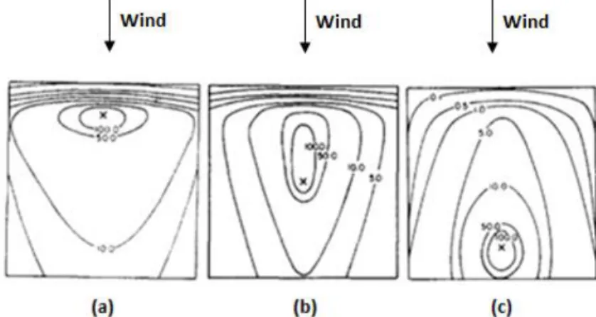
Li and Meroney [7] created a reduced-scale model of an isolated cubic building with a rooftop vent releasing pure helium (he). Several wind directions and distinct vent positions on the rooftop have been tested aiming to measure the pollutant concentration field. Results focus the influence of those different wind directions and distinct vent positions on the rooftop recirculation of the wind flow (Figure 2.4) and recirculation behind the building. (Figure 2.5-2.6).

Figure 2.4 Pollutant concentration K on the rooftop for different rooftop vent locations represented as ―x‖ (adapted from [7]): (a) located upwind; (b) located at the rooftop’s centre; (c) located downwind

Figure 2.5 Two dimensional perspective behind the building of the pollutant concentration K with vent located at the rooftop's centre (Figure 2.4(b)) (adapted from [7])

Figure 2.6 Side perspective of the pollutant concentration K behind the building with vent located at the rooftop's centre (Figure 2.4(b)) (adapted from [7])

The concentration of pure helium was quantified by the dimensionless concentration coefficient K obtained through the following equation and shown by isolines in Figure 2.4-2.6:

𝐾 =𝑐𝑈𝑏𝐻𝑏2

𝑄𝑒 (10)

K: dimensionless concentration coefficient [-] c: mass fraction of the pollutant [-]

Ub: wind velocity at reference building height Hb [m/s]

Hb: building height [m]

Qe: emission rate of the pollutant [m 3

Table 2.2 Parameters for defining the computational domain [7]

Parameter Description Value

α power-law exponent [-] 0.19

H domain height [m] 0.30

Hb building reference height [m] 0.05

Ub mean velocity in x-direction at reference height Hb [m/s] 3.30

Uref mean wind velocity at reference height [m/s] 4.50

Qe emission rate of the pollutant [m3/s] 0.0000125

z0 Ground aerodynamic roughness length [m] 0.0000750

Some parameters for defining the computational domain and boundary conditions from Li and Meroney [7] are shown in Tabe 2.2. Figure 2.7 and Figure 2.8 show the turbulence intensity (Iu) and

dimensionless wind-speed (U/Uref), respectively. For numerical simulation, both profiles have been

used to define the wind-speed and turbulence ones at the inlet and outlet the domain.

Figure 2.7 Turbulence intensity, Iu (%) (adapted from [7])

Figure 2.8 Dimensionless mean wind-speed (adapted from [7]) 0 0.2 0.4 0.6 0.8 1 0 10 20 z/ H [ -] Iu[%] 0 0.2 0.4 0.6 0.8 1 0 0.5 1 1.5 z/ H [ -] U/U_ref[-]

Figure 2.9 (a) Perspective view of geometry of Niigata's urban area and (b) measurement points location [8-10] Tominaga et al. [8] developed wind-tunnel experiments using a reduced-scale model of an actual urban area of Niigata city, Japan. A perspective view of geometry of that urban area is presented in Figure 2.9 (a). Measurements of the wind flow field were conducted in eighty reference locations distributed in the urban environment as shown by Figure 2.9 (b). The wind flow field was measured 0.008 m high at reduced-scale which means 2 m at full-scale aiming to perform those measurements at the pedestrian-level.

For the same model configuration, the Architectural Institute of Japan (AIJ) [9] set a pollutant source releasing ethylene (C2H4) near the centre of the urban area. Then, measurements for both wind

flow (Figure 2.10) and pollutant concentration field (Figure 2.11) were conducted quantifying the pollutant concentration by using concentration coefficient K already focused in the experiments of Li and Meroney [7]. Measurements were performed for four wind directions without modifications on the model. Those results presented in Figure 2.10-2.11 were measured from west wind direction.

. 0 0.5 1 1.5 1 4 7 10 13 16 19 22 25 28 31 34 37 40 43 46 49 52 55 58 61 64 67 70 73 76 79 Us /U re f [-]

Measurement point no.

0.0 0.1 0.2 0.3 0.4 0.5 1 4 7 10 13 16 19 22 25 28 31 34 37 40 43 46 49 52 55 58 61 64 67 70 73 76 79 K [-]

Measurement point no.

Figure 2.11 Concentration K (data provided by AIJ)

2.3.2 Numerical studies

All the wind-tunnel experiments previously referred [7,8] have provided results that are able for validating results of CFD simulations conducted with similar model configuration (Figure 2.12).

Many authors [6, 17-20] have based on experimental measurements [7] for predicting the pollutant concentration in a similar isolated cubic building by using CFD simulation, testing the sensibility of those results with several turbulence models and different pollutant source positions.

Figure 2.12 From the case study 2 performed by Gousseau et al. [6]. (a) Computational domain; (b) grid view (total number of cells: 1,480,754)

The most part of the authors [6, 17-20] have focused into analyse recirculation of the wind flow on the rooftop of the building as shown in Figure 2.13. That recirculation can cause backflow opposite the wind direction as consequence of the vortices on the rooftop, sides and behind the building (Figure 1.2-1.4). Recirculation and backflow are warnings for the reinjection of pollutants to inside the buildings and their high amount of concentration around the buildings at the pedestrian-level. High quantities of air pollution are harmful for the human's well-being, influencing his health and productivity negatively.

Figure 2.13 Side perspective of the vent at the rooftop's centre. (a) Wind-speed and recirculation of the flow (b) Pollutant concentration K going on the opposite direction of the wind flow because of the backflow promoted by the recirculation on the rooftop [1]

Numerical simulation results of the pollutant concentration on the rooftop and behind the building are shown in Figure 2.14-2.16.

Figure 2.14 Pollutant concentration K on the rooftop: (a) Wind-tunnel measurements by Li and Meroney [7]. (b-i) CFD results by: (b-d) Wang [17]; (e-g) Tominaga and Stathopoulos [18]; (h) Blocken et al. [19]; (i) Tominaga and Stathopoulos [20]. Results are presented for different turbulence models and turbulent Schmidt numbers, Sct. CS is the roughness constant [1]

Some cases were not able for reproducing recirculation on the rooftop because the turbulence model's limitations as shown in Figure 2.14 (e). Other cases can reproduce recirculation with different level of precision. The turbulent Schmidt number significantly influences some turbulence k-ε models as shown by a side-by-side comparison between both Figure 2.14 (f) and Figure 2.14 (h). The turbulence model approach has also a big influence on the results with special attention to Figure 2.15 (f) and 2.16 (f) that both resulted from LES simulation.

Figure 2.16 Side perspective of the pollutant concentration K behind the building (a) for the experiments conducted by Li and Meroney [7] and (b)-(f) for different turbulence models performed by Gousseau et al. [6]

CFD simulation has been conducted to predict pollutant concentration in urban areas as well. The study of the downtown of Montreal, Canada, was conducted by Stathopoulos et al. [21] through a reduced-scale model and, more recently, Gousseau et al. [22] have performed CFD simulation for the same model configuration which are validated with such results from Stathopoulos et al. [21].

A side-by-side comparison between reduced-scale models and grid arrangements is being presented in Figure 2.17 and Figure 2.18, for both southwest (SW) and west (W) wind direction.

Figure 2.17 Side-by-side comparison between both southwest wind-tunnel model and computational domain [22]

Figure 2.18 Side-by-side comparison between both west wind-tunnel model and computational domain [22] Measurements and predictions were made for fifteen reference positions as presented in Table 2.3. Pollutant concentration is quantified to hundred times the concentration coefficient K (100K). Several turbulence models were focused and a sensibility analysis of the turbulent Schmidt number was made with the Standard k-ε model.

Table 2.3 Dimensionless concentration (100K) and relative error values at each measurement point for the southwest direction [22] Point No. 100K (EXP) Standard k-ε model Sct=0.3 Standard k-ε model Sct=0.5 Standard k-ε model Sct=0.7 LES 100K %error 100K %error 100K %error 100K %error

1 27 20.2 25.2 13.4 50.4 7.7 71.5 12.6 53.3 2 32 32.7 2.2 23.9 25.3 15.1 52.8 16.2 49.4 3 57 70.1 23.0 53.9 5.4 34.3 39.8 27.8 51.2 4 71 69.7 1.8 62.3 12.3 50.0 29.6 32.7 53.9 5 60 125.5 109.2 104.2 73.7 78.6 31.0 47.8 20.3 6 104 174.2 67.5 124.0 19.2 68.8 33.8 38.1 63.4 7 68 62.4 8.2 68.5 0.7 66.9 1.6 30.5 55.1 8 96 90.5 5.7 91.6 4.6 84.3 12.2 42.1 56.1 9 131 1972.8 1406.0 797.7 508.9 365.2 178.8 227.3 73.5 10 79 59.5 24.7 74.0 6.3 81.7 3.4 31.3 60.4 11 69 73.5 6.5 82.5 19.6 87.8 27.2 40.0 42.0 12 120 77.7 35.3 70.6 41.2 69.2 42.3 43.1 64.1 13 59 77.1 30.7 37.9 35.8 23.2 60.7 52.4 11.2 14 925 314.3 66.0 624.2 32.5 858.3 7.2 439.7 52.5 15 1050 354.0 66.3 548.2 47.8 596.0 43.2 327.2 68.8

The concentration level of pollutants around the source are shown through Figure 2.19 for the southwest wind direction experiments. Differences between the turbulence models occur in respect to the pollutant concentration distribution, however recirculation of the wind flow is reproduced with both. The correlation between experimental and predicted results is quantified through the plots presented in Figure 2.20 with fair agreement.

Figure 2.19 Contours of the pollutant concentration 100K near the source for the southwest direction obtained with (a) Standard k-ε model (Sct = 0.7) and (b) LES [22]

Figure 2.20 Correlation of 100K for the southwest results by using (a) Standard k-ε model and (b) LES in comparison with experiments [22]

2.4

Quantification of agreement between the results

Aiming to quantify the agreement between experimental (E) and predicted (P) results are proposed the following statistical factors FB, NMSE, FAC2 and R [23]. N indicates the total amount of data, i the index of the value in the data and σE and σp the standard deviation of experimental (E)

and predicted (P) values respectively.

𝐹𝐵 = 𝐸 −𝑃 0.5(𝐸 +𝑃 ) (11) 𝑁𝑀𝑆𝐸 = 𝐸 𝑖−𝑃𝑖 ² 𝐸 𝑃 (12) 𝐹𝐴𝐶2 = 1 𝑁 𝑛𝑖→ 𝑛𝑖 = 1, 0.5 ≤𝑃𝑖 𝐸𝑖 ≤ 2 0, 𝑒𝑙𝑠𝑒 𝑁 𝑖=1 (13) 𝑅 =[ 𝐸𝑖−𝐸 (𝑃_𝜎 𝑖−𝑃 )] 𝐸𝜎𝑃 (14)

Fractional Bias (FB) quantifies systematic errors while Normalized Mean Square Error (NMSE) both the systematic and unsystematic ones. The ideal value is set to be zero which means no errors at all.

Fraction of Predictions within a factor of 2 of observations (FAC2) quantifies the number of data that is inside the range [0.5;2] considered acceptable for the ratio between predictions (P) and experimental results (E). Thus, in a perfect scenario FAC2 would be one meaning one hundred per cent of data inside the range. The correlation coefficient (R) consists in the linear relationship for both predicted (P) and experimental (E) results. R would also be one in a perfect scenario.

3. Case 1: Pollutant dispersion around an isolated cubic building

3.1

Experimental setup

3.1.1 Description

Li and Meroney [7] created a reduced-scale model of an isolated cubic building with a rooftop vent releasing pure helium (he). Several wind directions and distinct vent positions on the rooftop have been tested aiming to measure the pollutant concentration field. Results focus the influence of those different wind directions and distinct vent positions on the rooftop recirculation of the wind flow (Figure 2.4) and recirculation behind the building. (Figure 2.5-2.6). The concentration of pure helium was quantified by using the dimensionless concentration coefficient K (10).

3.1.2 Results

Figure 2.4 show a significant level of recirculation on the rooftop which forms backflow

opposite the wind direction. Behind the building, Figure 2.5-2.6 present lower concentration than on the rooftop. Indeed, at the pedestrian-level behind the building, concentration level is becoming lower.

3.2

CFD simulations

Case 1 aims to predict both the wind flow and pollutant concentration field which involves an isolated cubic building with a rooftop vent releasing pure helium (he). From west wind direction, several RANS turbulence models are tested. Predictions from Case 1 will be validated by comparisons against the wind-tunnel measurements from Li and Meroney [7] whose model configuration and input conditions are the base of the present case study.

Generally, numerical simulations with RANS equations require less computational resources and time than simulations with LES. Therefore, simulation with RANS has been conducted to generate an overview of the prediction accuracy of that turbulence model approach for the pollutant dispersion around isolated cubic buildings. The geometry is based on the experimental setup was performed by Li and Meroney [7] and previously presented. Those experiments have been used by different authors to assess the accuracy of numerical simulations in predicting pollutant concentration and to test the influence of the boundary conditions or other relevant parameters such as the wind direction, rooftop vent location or influence of the turbulent Schmidt number Sct [1,6,7].

The numerical assessment of the pollutant concentration will start by sizing the computational domain and creating a quality grid arrangement. Then, different turbulence k-ε models will be tested modeling first by using the RNG k-ε model. Predictions for both the turbulence Realizable k-ε model and RSM model will be also conducted. Based on the experimental setup and in the spatial discretization of the computational domain will be set the wind-speed and turbulence profiles and the boundary conditions. The west wind direction and a building configuration with a vent at the centre of the rooftop will considered in the present case study.

3.2.1 Model and computational domain

far from outlet of the domain. At the centre of the rooftop pure helium is being released from a circular exhaust vent.

Figure 3.1 Computational domain from Case 1. x/Hb indicates domain planes.

3.2.2 Computational grid

The spatial discretization of the computational domain should achieve a quality grid arrangement which can be assessed through the grid attributes skewness and stretching ratio. Based on those attributes, a quality grid was arranged with a total amount of 518,532 cells. It was made with the pre-processor Gambit 2.4.6.

All the domain was extruded from the ground-level up to the domain's height established (6Hb). Then, the internal volume of the building (Figure 3.2) were entirely deleted from the

ground-level to the building’s height (Hb) in order to set it as a wall [14].

Figure 3.2 Perspective view of part of the grid arrangement from Case 1. Wind direction is indicated by the arrow (518,532 cells).

The circular rooftop vent arranged on the rooftop’s face was modeled as a velocity inlet. Around it, 180 cells were defined in order to mesh the internal part of the vent. This is the finest meshed part of the entire domain.

Part of the computational grid is presented by Figure 3.2. Also fine mesh was arranged near the roof, front, side and back wall where the wind flow separation and recirculation occurs (Figure 1.2-1.4) [11,12].

Both Figure 3.3 and Figure 3.4 show Gambit perspective views of the grid arrangement. Figure 3.5 shows that grid in the internal part of the rooftop vent (a), and the quality of the cell's shape

(b) in a qualitative scale from 0 to 1 in which 0 is the best cell and 1 is the worst one. From those Figure 3.5 (a) and (b), it is possible to observe that, in general, inside and around the rooftop vent is being provided a quality grid arrangement.

Figure 3.3 Horizontal section of the computational domain

3.2.3 Boundary conditions

Before initializing any simulation, conditions should be set for characterizing the domain boundary conditions at the inlet, outlet, bottom, top and side walls. Also the rooftop vent, top and side walls of the building require boundary conditions for defining the pollutant released and turbulence associated to the source's geometry. Those boundary conditions were defined as expressed in Table 3.1.

Table 3.1 Boundary conditions from Case 1

Inlet

Velocity inlet

Momentum: Velocity magnitude U(z) Turbulence: k(z), ε(z)

Outlet

Pressure outlet

Static/Gauge pressure (Pa): 0 Turbulence: k(z), ε(z)

Bottom Wall, Shear condition: no slip

Wall roughness: z0=0.000075 m, Cs>1 (UDF: Cs=3.7), kS = 0.00020 m

Top Symmetry

Side Walls Symmetry

Rooftop vent

z-velocity: 0.627 m/s

Turbulence: Intensity and Length scale Turbulence intensity: 11.8%

Turbulence length scale: 0.00035 m Species: helium; Mass fraction: 1

Top and side walls of building

Wall

Shear condition: no-slip

Wall roughness: ks=0.0m; Cs=0.5

The wind flow and turbulence profile at the inlet and outlet are based on the measurements of the mean wind-speed and turbulence intensity (Figure 2.7-2.8) from Li and Meroney [7]. The wind flow was obtained by multiplying the mean wind-speed U/Uref (Figure 2.7) by Uref. The turbulent

kinetic energy k was calculated by the following equation as function of the domain's height [12] from the turbulence intensity Iu (Figure 2.8):

𝑘(𝑧) = (𝐼𝑢(𝑧)𝑈(𝑧))2 (15)

The turbulence dissipation rate ε(z) was imposed at the inlet through a user-defined function (UDF) from the equation (6) (see Annex I). The Von Kárman constant, к, was set to 0.42 and the friction velocity, u*, was established 0.22 m/s, according to previous studies using the same geometry. The wind flow and turbulence profile are then presented in Figure 3.6-3.8. Also a set of relevant parameters presented in Table 3.2 was used from the experimental setup for calculating the boundary conditions.

Figure 3.6 Mean wind velocity at the inlet from Case 1

Figure 3.7 Turbulent kinetic energy at the inlet from Case 1 0 0.1 0.2 0.3 0.4 0.5 0.6 0.7 0.8 0 1 2 3 4 5 z/ H x-velocity [m/s] Inlet 0 0.1 0.2 0.3 0.4 0.5 0.6 0.7 0.8 0 0.05 0.1 0.15 0.2 z/ H

Turbulent kinetic energy [m²/s²]

Inlet 0 0.1 0.2 0.3 0.4 0.5 0.6 0.7 0.8 0 1 2 3 4 5 z/ H

Turbulence dissipation rate [m²/s³]

Table 3.2 Model parameters for calculating the boundary conditions

Parameter Description Value

α Power-law exponent 0.19

Hb Building reference height [m] 0.05

Dv Exhaust diameter [m] 0.005

UH Mean velocity in x-direction at reference height Hb [m/s] 3.30

We Exhaust velocity [m/s] 0.627

Me Exhaust momentum ratio 0.19

Av Exhaust surface [m²] 0.00002

Qe Emission rate of the pollutant [m³/s] 0.00001

At the bottom were defined both wall shear condition (no slip) and wall roughness. Wall roughness requires definition of the surface roughness length z0 and the roughness constant Cs. z0 has

been set by Li and Meroney [7] and it has also been used by other authors for the presented model configuration [6,17-20]. However, Cs directly depends on the grid arrangement. Then, it is possible to

calculate Cs by using equation (8) and the statement ks<yp [13,16]. ks is the physical roughness height

of the bottom and yp corresponds to half the height of the grid first cell. Therefore, yp was set to

0.00023 m and ks equal to 0.00020 m for assuring that relationship ks<yp. From (8) Cs is set to 3.7. As

Cs> 1, an user-defined function (UDF) for setting the value of the constant Cs is required because it is

out of the range [0;1] (see Annex 1) [16]. Both the top and side walls of the computational domain were set as symmetry which means no boundary conditions were defined at these planes because there is no flux of any quantity [13].

The rooftop vent was modeled by defining an exhaust vertical velocity, We, the turbulence

intensity and length scale and the pollutant (pure helium). We was defined through the momentum

ratio Me [7]. Me is equal to 0.19 and is a ratio between the exhaust vertical velocity We and the velocity

at the reference height which means building's height 3.3 m/s. Then, We was set to 0.627 m/s.

The turbulence intensity Iu, which is a measured value at the inlet boundary, has been stated

by Li and Meroney [7] to 11.8%. The turbulence length scale Lt was set 0.07 times the rooftop vent

diameter [13] from equation (9).

Top and side walls of the building were set to default walls keeping the shear condition and wall roughness as recommended [13].

3.2.4 Other relevant parameters and settings

Besides the boundary conditions, discretization schemes have to be selected in spite of their influence in RANS simulations is smaller. Those schemes are presented in Table 3.3. Generally, second-order scheme is able to achieve higher accuracy than the first-order one [13]. The maximum degree of convergence was set to 10-11 for all the variables.

Table 3.3 Discretization schemes

Discretization

Pressure-velocity coupling: SIMPLE (Semi-Implicit Method for Pressure-Linked Equations)

Pressure: Second order

Momentum, k and ε: Second order upwind Helium, Energy: Second order upwind

3.3

Comparison experiments with simulations

A side-by-side comparison between the experimental and predicted results of the Case 1 will be presented. Also the "case study 2" from Gousseau et al. [6] will be focused for comparison once it was treated the same building model configuration.

Figure 3.9 Case 1: X-velocity (a) vertical plane (side view) and (b) horizontal plane (top view)

Results from Case 1 are then reported. Figure 3.9 shows the velocity contours in the x-direction for both vertical (a) and horizontal perspective (b). It is possible to identify the wind flow separation zone and stagnation region in front of the building, recirculation on the rooftop, sides and behind the building by comparing Figure 3.9 (a) against Figure 1.2-1.4. Recirculation causes backflow opposite the wind direction as demonstrated by the experimental results in Figure 3.10 (a). Predicted results [6] present fair agreement against the experiments, in spite of overpredicted.

From Case 1, pollutant concentration contours on the rooftop are significantly underpredicted in relation to the experimental setup [7]. However, recirculation of the flow is clear on the rooftop Figure 3.10 (c).

Pollutant concentration predictions were also performed at the pedestrian-level, behind the building as shown in Figure 3.11. Case 1 still reproduces concentration levels with significant underprediction at this region (Figure 3.11(a)). In general, Gousseau et al. [6] overpredicted them in Figure 3.11 (b), however their results show better agreement to the experiments (Figure 3.11(c)) than the ones provided by Case 1.

Figure 3.11 Pollutant concentration K contours at the pedestrian-level behind the building (a) from Case 1, (b) by Gousseau et al. [6] and (c) by Li and Meroney [7]. Both (b) and (c) was calculated by using RANS RNG k-ε model.

Figure 3.12-3.15 corroborate the underprediction of those results shown previously. The plots presented only provide comparisons between Case 1 and the experimental measurements since Gousseau et al. [6] do not provide such results. Figure 3.12 analyse the pollutant concentration at the ground-level behind the building. This region was already focused in Figure 3.11 for analysing concentration in heights higher than the ground. Now, observing the ground-level results, values are not changing significantly which means that Case 1 is still underpredicted.

Pollutant concentration on the top edge behind the building at x/Hb=1 (Figure 3.13) show fair

agreement between Case 1 and the experiments. However, between y/Hb=-05 and y/Hb=0.5, mainly in

the centre (y/Hb=0) this agreement becomes poor. Here, pollutant concentration predictions are

Figure 3.12 Pollutant concentration K predictions at the ground-level behind the building

Figure 3.13 Pollutant concentration K predictions in the edge (1) behind the building at x/Hb=1

On the boundaries of the building, pollutant concentration is analysed as well. Based on the numerical study [19] both rooftop and back’s centreline are on focus (Figure 3.14-3.15). On the rooftop, recirculation level is slightly underpredicted and not that gradual as should be based on the experimental results. Concentrations change suddenly from 660 (x/Hb=0) to 100 (x/Hb=-0.12). From

wind-tunnel experiments, concentration level 100 is achieved on the rooftop’s centerline at x/Hb

=-0 0.1 0.2 0.3 0.4 0.5 0.6 1 2 3 4 5 K [ -] x/H_b[-]

Wind Tunnel Case 1

0 0.5 1 1.5 2 2.5 3 3.5 -2 -1.5 -1 -0.5 0 0.5 1 1.5 2 K [ -] y/H_b [-]

Figure 3.14 Pollutant concentration K on the rooftop's centreline

Figure 3.15 Pollutant concentration K on the back's centreline behind the building

3.4

Sensitivity analysis

3.4.1 Grid-sensitivity

It is recommended that the grid-sensitivity should be tested in order to guarantee that results do not change significantly with more or less cells for the same model configuration [11,12]. Therefore, a grid-sensitivity analysis was performed increasing the total amount of cells. As recommended by Franke et al. [11] and Tominaga et al. [12], a factor of √2 was set to increase the

0 100 200 300 400 500 600 700 -0.5 -0.4 -0.3 -0.2 -0.1 0 0.1 0.2 0.3 0.4 0.5 K [ -] x/Hb[-]

Wind Tunnel Case 1

0 0.2 0.4 0.6 0.8 1 0 1 2 3 4 5 z/ Hb [-] K [-]

number of cells that compose every single edge. Then, the finest grid achieved a total amount of 1,701,080 cells. A comparison between both coarser and finer grid can be made by observing Figure 3.16. After performing simulations by using the turbulence RNG k-ε model for both grids and using the same boundary conditions as well, it was concluded that those results did not change significantly. Thus, the coarsest grid was selected for performing new simulations with different turbulence models.

Figure 3.16 Grid arrangements: Coarse grid 518,532 cells (a-b) and Fine grid 1,701,080 cells(c-d); (a) and (c) show the side, back and top of the building; (b) and (d) show a closer top view of the building

In general, there is no large discrepancies between both coarser and finer grid. Pollutant concentration contours on the rooftop (Figure 3.17) and behind the building (Figure 3.18-3.19) have shown fair agreement.

Some discrepancies occur behind the building at the building's height as shown in Figure 3.20. Mainly in the range -0.5<y/Hb<0.5, Hb far the building, the finest grid show higher levels of

concentration than the coarsest one which means more accuracy when comparing against the experimental results presented through Figure 2.5. Both pollutant concentration predictions on the rooftop's and back's centreline show no discrepancies (Figure 3.21-3.22). As the coarsest grid requires less time-consuming, it was selected for testing more turbulence models. Those results will be presented in the following sections.

Figure 3.18 Comparison of pollutant concentration K contours behind the building. Continuous line is the coarsest grid; Dashed line corresponds to the finest grid.

Figure 3.19 Comparison of pollutant concentration K predictions at the ground-level behind the building 0 0.02 0.04 0.06 0.08 0.1 0.12 0.14 1 2 3 4 K [ -] x/Hb[-]

Figure 3.20 Comparison of pollutant concentration K predictions in the edge (1) behind the building at x/Hb=1 (Hb far the building)

Figure 3.21 Comparison pollutant concentration K on the rooftop's centreline 0 0.1 0.2 0.3 0.4 0.5 0.6 0.7 -1.5 -1 -0.5 0 0.5 1 1.5 K [ -] y/Hb[-]

Coarse grid Fine grid

0 100 200 300 400 500 600 700 0 0.1 0.2 0.3 0.4 0.5 0.6 0.7 0.8 0.9 1 K [ -] x/Hb[-]

Figure 3.22 Comparison of pollutant concentration K on the back's centreline behind the building

3.4.2 Influence of turbulence models: RNG k-ε model, Realizable k-ε model

and RSM

In the previous section, it was presented results simulating with RANS by using the turbulence RNG k-ε model. Two more RANS turbulence models were tested, the Realizable (RLZ) k-ε model and Reynolds-stress model (RSM). The calculation conditions are similar with the RNG k-ε model. With the Realizable k-ε model the turbulent Schmidt number (Sct) was set to 0.7. Thus, comparison

with numerical results provided by Gousseau et al. [6] can be done against simulations from Case 1 once such turbulence models, both the wind flow and turbulence profiles and boundary conditions are all similar. Those results are compared through Figure 3.23-3-29 by presenting pollutant concentration contours on the rooftop (Figure 3.23), behind the building (Figure 24-27) and in both rooftop's centreline (Figure 3.28) and back's centreline behind the building (Figure 3.29).

In general, from Case 1, all the turbulence models achieved underpredicted results in relation to the simulation results from Gousseau et al. [6] and the experimental setup [7].

On the rooftop and at the ground-level behind the building, Case 1 presents fair agreement between the three turbulence models in respect to the pollutant dispersion patterns (Figure 3.23-27), in spite of the underprediction already demonstrated against both numerical and experimental results provided [6,7].

In the pollutant concentration predictions Hb far behind the building (Figure 3.27), RLZ k-ε

model offers the best prediction when compared against the experiments [7]. Figure 3.27 shows that both RNG k-ε model and RSM present results significantly underpredicted in relation to RLZ k-ε model and experiments [7].

In spite of good agreement presented in Figure 3.27, RLZ k-ε model have not been able to reproduce recirculation opposite the wind direction on the rooftop. Both RNG k-ε model and RSM are more accurate at that point as shown in Figure 3.28. Pollutant concentration on the back's centreline behind the building is more accurately predicted by the RLZ k-ε model near the top of the building (Figure 3.29) once again, however it is not that significant. Nevertheless, all turbulence models are still underpredicting the pollutant concentration, in spite of correctly reproducing the pollutant dispersion patterns around the building, mainly both the RNG k-ε model and RSM.

0 0.25 0.5 0.75 1 0 0.5 1 1.5 2 2.5 3 3.5 4 4.5 5 z/ Hb [-] K [-]

Figure 3.23 Comparison of pollutant concentration K contours on the rooftop: (a)-(c), RNG k-ε model, RLZ k-ε model and RSM from Gousseau et al. [6], respectively; (d)-(f) RNG k-ε model, RLZ k-ε model and RSM from Case 1, respectively. Note that in (b), the dash-dot line represents RLZ k-ε model with a Schimdt number of 0.7 which it is the one taken into account.

Figure 3.25 Pollutant concentration K contours behind the building (a) RSM from Case 1 and (b) RSM from Gousseau et al. [6]

Figure 3.26 Pollutant concentration predictions at the ground-level behind the building 0 0.1 0.2 1 2 3 4 K [ -] x/Hb[-]

Figure 3.27 Pollutant concentration predictions in the edge (1) behind the building at x/Hb=1 (Hb far the building) 0 0.5 1 1.5 2 2.5 3 -1 -0.75 -0.5 -0.25 0 0.25 0.5 0.75 1 K [ -] y/Hb[-]

Wind Tunnel Case 1 RNG Case 1 RLZ Case1 RSM

0 100 200 300 400 500 600 700 0 0.25 0.5 0.75 1 K [ -] x/Hb[-]

Figure 3.29 Pollutant concentration K on the back's centreline behind the building

3.4.3 Influence of turbulent kinetic energy (k)

It would be expected to achieve the same results and not such underprediction in relation to the numerical [6] and experimental results [7] from the other authors. Thus, in order to understand which kind of influence turbulence can have on the recirculation and pollutant dispersion at the rooftop level and behind the building, simulations were performed using different turbulent kinetic energy k profiles obtained by multiplying the original k values by the factors 0.25, 0.5 and 2 which means reduction of 25% and 50% and increasing of 100%. Simulations were performed with turbulence RNG k-ε model.

Figure 3.30 (a) shows the experimental pollutant concentration contours on the rooftop [7] and Figure 3.30 (b) the results obtained by Gousseau et al. [6] with the RNG k-ε model. From Case 1, by using the RNG k-ε model as well, Figure 3.30 (c)-(f) presents respectively 0.25k, 0.5k, k and 2k profiles. 0.25k presents the most accurate results and the closest ones to the numerical [6] and experimental [7] results. Also in Figure 3.31, 0.25k presents higher predictions behind the building by correctly reproducing the pollutant dispersion patterns, however their underprediction persists.

Figure 3.32 shows the pollutant concentration predictions on the rooftop's centreline as shown previously. It was clear that a considerable impact on the recirculation region exists by using different k profiles. The 0.25k profile can more accurately predict the recirculation level and pollutant dispersion values opposite the wind direction in relation to the experimental results [7]. On the other hand, the 2k profile presents the worst results. This can evidence discrepancies in the calculation of the turbulent kinetic energy k profile between both Case 1 and Gousseau et al. [6]. On the back's centreline different turbulent kinetic energy k profiles present no large discrepancies and, consequently, the agreement with the numerical [6] and experimental [7] results was not improved (Figure 3.33).

Then, it is clear that turbulent kinetic energy k has a big influence on the recirculation at the rooftop level and, there, it could have influenced the results from Case 1. In fact, with the 0.25k profile, the results provided by Gousseau et al. [6] are not better than Case 1 ones for the isolines K=50 and K=100 as shown in Figure 3.30 (a)-(c). Behind the building its influence is not that big. As expressed in Figure 3.31 and Figure 3.33, the results are not significantly improved by using different turbulent kinetic energy profiles.

0 0.25 0.5 0.75 1 0 1 2 3 4 5 z/ Hb [-] K [-]

Figure 3.30 Side-by-side comparison of pollutant concentration K contours on the rooftop: (a) Experimental [7]; (b) Numerical [6]; (c)-(f) Results from Case 1 for 0.25k, 0.5k, 1k and 2k, respectively

Figure 3.32 Comparison pollutant concentration on the rooftop's centreline for the several turbulent kinetic energy k profiles

Figure 3.33 Concentration on the back's centreline behind the building for the several turbulent kinetic energy k profiles

3.5

Discussion and conclusion

Based on the previous numerical [6] and experimental [7] results for a similar model configuration, Case 1 has been developed. A computational domain sufficiently wide and a quality grid arrangement were created for simulating an isolated cubic building releasing pure helium from a rooftop vent located 0.05 m high. Also the boundary conditions were set based on those previous studies [6,7]. 0 100 200 300 400 500 600 700 0 0.1 0.2 0.3 0.4 0.5 0.6 0.7 0.8 0.9 1 K [ -] x/Hb[-] 1k 0.5k 0.25k 2k Wind Tunnel (1k) 0 0.25 0.5 0.75 1 0 0.5 1 1.5 2 2.5 3 3.5 4 4.5 5 z/ Hb [-] K [-] 1k 0.25k 0.5k 2k Wind Tunnel

A grid-sensibility analysis was conducted aiming to test the influence of a higher number of cells in the simulation results achieved. As shown through Figure 3.17-3.21, the finest grid presented no large influence on the results and the coarsest one was selected to perform more simulations.

Aiming to assess the recirculation of the wind flow and pollutant concentration on the rooftop and behind the building, three turbulence models have been used such as Realizable k-ε model, RNG k-ε model and Reynolds-stresses model (RSM). The pollutant concentration was underpredicted by all of those turbulent models. However, the pollutant dispersion patterns with RNG k-ε model and RSM have presented fair agreement on both the rooftop and behind the building. This results of the accuracy of those turbulence models in predicting the recirculation, mainly on the rooftop (Figure 3.23).

Such underprediction of the results led to test kind of influence turbulence can have on the recirculation and pollutant concentration on the rooftop level and behind the building. Simulations were performed with the turbulence RNG k-ε model by using different turbulent kinetic energy k profiles obtained by multiplying the original k values by the factors 0.25, 0.5 and 2. It was concluded that lower k profiles can more accurately predict the recirculation on the rooftop while higher ones cannot, presenting worse results inclusively.