Detection and Classification of Obstacles for Autonomous Vessels Using Machine Learning

F

E

U

P

Detection and Classification of

Obstacles for Autonomous Vessels Using

Machine Learning

António Pedro Rodrigues Pereira

MASTER’S DEGREE INELECTRICAL ANDCOMPUTERSENGINEERING Supervisor: José Carlos dos Santos Alves

c

Resumo

Sistemas de deteção de obstáculos têm sofrido grandes avanços nos últimos anos devido ao desen-volvimento de veículos autónomos. Apenas com estes sistemas é possivel garantir a integridade dos mesmos. Particularmente no desenvolvimento de embarcações autónomas, estes sistemas passam pela fusão de sensores como Radar, Lidar e câmaras de forma a que a embarcação con-siga operar mesmo em situações de clima adverso. Com o grande desenvolvimento das câmaras de vídeo, impulsionado pelo mercado de telemóveis, o recurso a câmaras de vídeo apresenta inúmeras vantagens para sistemas de deteção de obstáculos.

Esta dissertação pretende avaliar a performance de um sistema de deteção de obstáculos re-orrendo apenas a câmaras de vídeo, usando técnicas de visão por computador e machine learning para atingir esse fim. Inicialmente é feita uma revisão das várias técnicas de processamento de imagem tradicionais e algoritmos baseados em deep learning.

A solução proposta é constituída por dois módulos, um detetor de objetos baseado no algoritmo "You Only Look Once" e um detetor da linha do horizonte constítuido por uma rede neuronal, de forma a que cruzando a informação destes dois módulos, seja possível extrair informação acerca da distância relativa dos obstáculos detetados. Esta solução consegue detetar 70.1% dos obstáculos presentes no dataset, conseguindo processar frames em tempo real. A estimação da linha do horizonte atinge uma precisão de 97.9% demorando 20ms a prever um resultado. Apesar da solução não apresentar os melhores resultados na classificação dos obstáculos, é demonstrado que o uso de técnicas de machine learning têm melhores resultados comparativamente a técnicas tradicionais de processamento de imagem.

Abstract

Obstacle detection systems have undergone major advances in recent years due to the development of autonomous vehicles. Only with these systems is it possible to guarantee their integrity.

Particularly in the development of autonomous vessels, these systems resort to sensor fusion such as Radar, Lidar and video cameras so that the vessel can operate even in adverse weather situations, taking advantage of each sensor’s characteristics. With the extraordinary evolution of video cameras, driven by the mobile phone market, the use of this sensor type has many advantages for obstacle detection systems.

This dissertation intends to evaluate the performance of an obstacle detection system resorting only to video cameras, using computer vision and machine learning techniques to reach this end. Initially, is it presented a review on conventional image processing and deep learning algorithms for object detection.

The proposed solution consists of two modules, an object detector based on the "You Only Look Once" algorithm and an horizon-line detector, consisting of a neural network, so that by fusing the information of these two modules, it is possible to extract information about the relative distance of the detected obstacles. This solution detected 70.1% of the obstacles present in the dataset, managing to process frames in real-time. The estimate of the horizon line reaches an accuracy of 97.9% and takes 20 ms per frame to predict a result. Although the solution does not present the best results in obstacle classification, it is demonstrated that the use of machine learning techniques leads to better results when comparing with traditional image processing techniques.

Acknowledgements

I would like thank both my supervisors for all the help they have given me throughout this entire project. I would also like to thank my friends for all the support they have given me all these years. And I want to thank my family for everything they have done for me, but in particular, to both my parents. They were always there for me and I could not have done this without their support.

“Imagination is more important than knowledge. Knowledge is limited. Imagination encircles the world.”

Contents

2 State of the Art Review 3 2.1 Existing Solutions . . . 3 2.2 Obstacle Detection . . . 4 2.2.1 Background Subtraction . . . 4 2.2.2 Optical Flow . . . 5 2.3 Object Tracking . . . 6 2.4 Deep Learning . . . 7 2.4.1 Neural Network . . . 8

2.4.2 Convolutional Neural Network . . . 10

2.4.3 Object Detection using CNN . . . 11

2.4.4 Comparison between models . . . 14

2.5 Related Work . . . 14 3 Methodology 17 3.1 Proposed Solution . . . 17 3.1.1 Object Detection . . . 18 3.1.2 Horizon Detection . . . 19 3.2 Dataset . . . 23

3.2.1 Singapore Maritime Dataset . . . 23

3.2.2 Other Datasets . . . 26 3.3 Evaluation Metrics . . . 26 3.3.1 IoU . . . 26 3.3.2 Precision . . . 27 3.3.3 Recall . . . 27 3.3.4 mAP . . . 27 4 Experimental Setup 29 4.1 Environment . . . 29 4.2 Training Phase . . . 29

4.2.1 Train and Validation . . . 29

4.2.2 Object Detector . . . 30

x CONTENTS 4.3 Darknet Modifications . . . 32 5 Results 33 5.1 Object Detector . . . 33 5.1.1 Training Results . . . 33 5.1.2 General Performance . . . 34

5.1.3 Effect of target size . . . 35

5.1.4 Effect of image input dimensions . . . 36

5.1.5 Comparison with smaller architecture . . . 37

5.1.6 Comparison with Related Work . . . 38

5.2 Horizon Detector . . . 38

5.3 System Performance . . . 40

6 Conclusion and Future Work 43

A Detections Examples 45

List of Figures

2.1 Comparison between different available maritime sensors [1] . . . 4

2.2 Different tasks of Computer Vision. Extracted from [2] . . . 7

2.3 McCulloch-Pitts model of a neuron . . . 8

2.4 Common activation functions used in neural networks [3] . . . 9

2.5 General CNN architecture. Extracted from [4] . . . 10

2.6 R-CNN Flowchart. Extracted from [5] . . . 11

2.7 Fast-RCNN Architecture. Extracted from [6] . . . 12

2.8 Faster-RCNN Architecture. Extracted from [7] . . . 13

3.1 Proposed Solution Architecture . . . 17

3.2 YOLOv3 Network Diagram. Extracted from [8] . . . 18

3.3 Representation of the exhaustive search method . . . 21

3.4 Example of predicted horizon lines with region-based algorithm. . . 21

3.5 Illustration of Horizonet architecture . . . 22

3.6 Example of an horizon detection at 1920 × 1080 resolution . . . 22

3.7 Example of an horizon detection at 416 × 416 resolution . . . 23

3.8 Sample frames from the Oh-Shore videos in the SMD. . . 24

3.9 Sample frames from the Oh-Board videos in the SMD. . . 24

3.10 Sample frames from the NIR videos in the SMD. . . 24

3.11 Diagram of Object Ground Truth Data . . . 25

3.12 Diagram of Horizon Ground Truth Data . . . 26

5.1 Training output . . . 33

5.2 Example of detection with the trained network . . . 34

5.3 Inaccurate detection . . . 35

5.4 Ground truth detection of5.3 . . . 35

5.5 Average Precision Per Class . . . 36

5.6 Average Precision per size of the target . . . 36

5.7 Training results for Tiny-YOLOv3. . . 37

5.8 Training results of Horizonet . . . 39

5.9 Comparison of real and predicted horizon line. Green line represents the real horizon and the red line represents the prediction. . . 39

5.10 Horizon prediction within an hazy environment. . . 40

5.11 System detection example . . . 41

5.12 Perfect detection example from the On-Shore frames. . . 42

5.13 Poor detection due to miss prediction of the horizon line. However, the system is still able to infer the relative distances of the obstacles with some precision . . . 42

xii LIST OF FIGURES

A.1 Example of detection from Training Dataset. Possible to observe that in the

train-ing subset the network can identify the Ferry class. . . 45

A.2 Good detection example from testing subset. . . 46

A.3 Miss detection of an obstacle. . . 46

A.4 Perfect detection . . . 47

A.5 Miss classification example . . . 47

A.6 Bad horizon prediction on On-Board frame . . . 48

List of Tables

2.1 Comparison of speeds and performances for models trained with the 2007 and 2012 PASCAL VOC datasets. Results extracted from [9] and [10]. . . 15

2.2 Comparison of speeds and performances for models trained with the COCO dataset. Results extracted from [11] and [12] . . . 15

3.1 Information about the different object classes in the Singapore Maritime Dataset. 25

4.1 Frequency of each class within the test + train subsets . . . 30

5.1 Comparison of performance with image resolution . . . 37

5.2 Results from YOLOv3 and Tiny-YOLOv3 networks. . . 37

5.3 Comparison of background subtraction methods for object detection in a maritime environment. Results extracted from [13]. . . 38

Abbreviations and Symbols

ASV Autonomous Surface Vehicle AIS Automatic Identification System CNN Convolutional Neural Network DL Deep Learning

IoU Intersection over Union mAP Mean Average Precision YOLO You Only Look Once

SSD Single Shot Multibox Detector IR Infra-Red

TP True Positive FP False Positive FN False Negative AP Average Precision SVM Support Vector Machine ROI Region of Interest

RPN Region Proposal Network SMD Singapore Maritime Dataset IR Infra-Red

Chapter 1

Introduction

1.1

Context

Autonomous ships or ASVs (Autonomous Surface Vehicles) are a reality in today’s age for diverse types of operations such as environmental monitoring, resce missions, surveillance or even in military situations. The use of ASVs has several advantages when compared to manned vessels as it lowers the cost of the operation and enables operations that can have a serious risk for the human life. It also has great potential for surveillance operations as an ASV can have small dimensions.

The operation of autonomous ships in the marine environment requires systems that allow the detection and classification of obstacles of various types that may be subject to collisions and result in damages that require the manual recovery of the vehicle or even its total loss. Although an increasing number of conventional ships make use of the Automatic Identification System for Ships (AIS), which diffuses their position, course and speed within a few kilometers, smaller manned vessels, fisheries in our coastal waters and other types of floating or semi-submerged wrecks pose a significant potential risk that could jeopardize the operation of an autonomous vehicle.

1.2

Motivation

The maritime environment is extremely risky for autonomous operations due to extreme variability of the wind and sea and possible collisions with small fishing boats that do not possess an AIS system, buoys or even ships’ wreckage. This risk has to be mitigated with obstacle detection and evasion systems in order not to compromise the operation of the autonomous vessel.

In the last years, video cameras undergone an extraordinary evolution motivated by the mobile phone market in terms of resolution, energy consumption, dimension and cost. It is important to note that there are cameras that are sensible to non-visible wavelength, like thermal cameras, allowing the capture of images in weak or null visibility conditions.

A solution based only on video cameras for obstacle detection would present a large benefit over current available solutions, such as Radar, Lidar or Sonar. These available solutions have

2 Introduction

big physical dimensions and higher energy consumption when comparing them to a video camera, which makes it a desired solution for the navigation of ASVs.

1.3

Objectives

This project aims to implement a system for the detection and classification of obstacles (accord-ing to their size, shape and especially distance to the autonomous vessel) on the surface of the water using machine learning techniques applied to the image acquired by a camera video and complemented by data from other vehicle sensors, such as its longitudinal and transverse slope (roll and pitch angles), as well as its geographic orientation. The great variability of the quality of the images acquired on board in terms of ambient brightness and the state of the sea surface make this problem particularly difficult. In this work, it is intended to implement a solution that relies on a low-cost commercial monocular camera (webcam type or camera available for the Rasp-berryPi platform), which presents computing requirements compatible with standard embedded computing platforms (RaspberryPi or similar). It should be noted that such a system will also be interesting on board vessels operated by small crews as a means of alerting potential collision risks.

The objective of this work is to infer if an obstacle detection system based only on computer vision has better results over state of the art systems.

1.4

Dissertation Structure

This dissertation is divided into 6 chapters. The first chapter serves to contextualize the reader with the problem that this work intends to explore, giving more insight to the need for the safety of autonomous ship navigation. In chapter 2, it is presented the solutions currently available to address the problem and a theoretical discussion about the state of the art technology available to implement the desired solution. Chapter 3 contains a detailed explanation over the architecture of the proposed solution and why certain algorithms were chosen over other available solutions. The later chapters, namely chapters 4 and 5, serve to detsil how the experimental setup and how the results were achieved, as well as a discussion about the obtained results. The final chapter consists in the discussion of the conclusions over the obtained results and a brief discussion over possible future work.

Chapter 2

State of the Art Review

In this chapter, it is described all the related work done in the areas of segmentation, tracking and object classification in real-time, as well as deep learning techniques for real-time object detection.

2.1

Existing Solutions

For designing an obstacle detection system, there are a variety of sensors widely available. One historic widely used sensor is the radar. The radar was historically developed for military purposes before and during World War II and it is a detection system capable of determining the distance, angle or velocity of a target with radio waves. Radar capability is influenced by the operating band of the radar, where higher frequencies typically offer better angle and range resolution [1].

Another sensor used is the Light and Detection Ranging (LIDAR), which is a scanning laser sensor technology capable of providing really accurate distance measures. Differences in laser return times can be used to create a detailed 3-D mapping of the surrounding of the vehicle. How-ever, this sensor has some disadvantages when considering its use in harsh maritime environments, as it uses rapidly moving mechanical components for the scanning operation, which can be prone to malfunctions. The LIDAR range and accuracy can be also affected by adverse weather condi-tions, such as fog and rain [1].

In figure 2.1, it is shown a detailed comparison between several available maritime sensors. As it is possible to conclude, cameras are a good choice for an obstacle detection system, since they are cheap, are small-sized and durable and can provide high spatial information with color information that leads to object identification. However, it is difficult to extract the distance mea-surement of the obstacles using only one camera, which is one of the goals for this dissertation.

The challenge for this project is to build a real-time obstacle detection system that only uses a camera as its sensor and is able to not only detect an obstacle, but can also extract information about its relative distance to the camera. In order to achieve this goal, the next section highlights the state of the art algorithms.

4 State of the Art Review

Figure 2.1: Comparison between different available maritime sensors [1]

2.2

Obstacle Detection

In this section we will present a theoretical review of state-of-the-art algorithms that can be used for obstacle detection based purely on computer vision. It starts with a review from traditional image processing approaches for object detection and object tracking and later a review of object detection algorithms which use deep learning techniques.

2.2.1 Background Subtraction

To separate the foreground from the background, one frequently used technique in this context is background subtraction, as explained in [14] and [15]. Generally, background images contain ob-jects that remain static in the scene. The objective is to subtract that image from our current frame, highlighting the difference between the two frames and, therefore, identifying the foreground ob-jects as expected.

In [15], for every frame in a video sequence, the background is subtracted from the current image, originating a difference image, which is thresholded to give a binary object mask. All the pixels referring to the foreground objects have value 1 and all the pixels referring to background objects have value 0. This approach illustrates the general idea behind the background subtraction method and how the background model is computed.

However, this approach requires fixed camera setups and is sensible to non stationary back-grounds, like swaying trees or illumination changes.

The Background Subtraction approach can be divided in two categories: [16] [17] • Recursive Algorithms

2.2 Obstacle Detection 5

2.2.1.1 Recursive Algorithms

The Recursive algorithms do not maintain a buffer for the background modeling. This technique recursively updates a single background model based on each input frame, so the current model can be affected by frames from a distant past [18].

There are several methods included in recursive algorithms, such as Approximate Median method, where the running estimate of the median is incremented by one if the input pixel is larger than the estimate, and decreased by one if it is smaller. This estimate eventually converges to the median, containing values for which half of the input pixels are larger and half of the input pixels are smaller than this estimated value, as stated in [19].

Another example of a recursive algorithm is the Mixture of Gaussians, where each pixel location is represented by a number (or mixture) of gaussian functions that are summed together to form a probability distribution function [20].

In [21] are described other methods used to solve this problem. One of those methods is the use of predictive filters, such as Kalman or Wiener, to predict the background image in the next frame. These techniques strongly depend on the preset state transition parameters and fail in case the distribution does not fit into a single model or varies randomly.

A major shortcoming of the methods presented so far is that they neglect the temporal corre-lation among the previous values of the pixel. This prevents them from detecting a structured or periodic change.

To detect such backgrounds, one method used is the Wave-Back [22]. This algorithm detects new objects based solely on the dynamics of the pixels in a scene rather than their appearance. For a given frame, the frequency coefficients are computed and compared with the background coefficients to obtain the distance map, where it will be applied a threshold to determine the foreground pixels.

2.2.1.2 Non-Recursive Algorithms

The Non-Recursive approach is based on the sliding window concept for the background estima-tion. It uses a buffer to store the previous frames of the video and it estimates the background based on the temporal variation of each pixel within the buffer. [19]

The most common Non-Recursive method is Median Filtering, that consists in estimating the background as the median of all the frames stored in the buffer at each pixel location. [17]

2.2.2 Optical Flow

This technique consists on calculating the optical flow field of an image or video frame and per-form the clustering on the basis of the optical flow distribution inper-formation obtained from the image (video frame). This method allows in obtaining the complete knowledge about the move-ment of the object and is useful to distinguish moving targets from the background. A moving object in a scene can introduce image velocities that do not match with this pattern. This

incon-6 State of the Art Review

can help in segmenting images into regions that correspond to different objects [16]. However, due to the large number of calculations needed for this technique, it is not suitable for real-time applications.

2.3

Object Tracking

Tracking is locating a region corresponding to a moving object in a video sequence. Objects often change their appearance or pose. They occlude each other, become temporarily hidden, merge and split. Depending on the application, they exhibit erratic motion patterns and often make sudden turns.

In [15], it is described a method of tracking based on building an association graph. After successfully detecting an object, its region is extracted within each frame, allowing for the tracking of the given object and extracting information like velocity and distance. But as regions can split, merge, randomly disappear, the region tracking method must be able to work reliably even in the presence of such events.

The association graph is a bipartite graph where each vertex corresponds to a region. All the vertices in one partition of the graph correspond to the previous frame, P and all the vertices on the other partition correspond to regions in the current frame, C. An edge, E, between two vertices, Vi

and Vj indicates that the previous region Piis associated with the current region Ci.

The region extraction set is done for each frame, resulting in new regions detected, that will become the current regions, C. The current regions C in frame i will become the previous regions P in frame i + 1. To make and edge between a current region C and a previous region P, it is calculated the area of intersection of P and C to weight the edge. The objective is to find the maximal weight graph.

Another tracking method, described in [23], is the use of both temporal differencing and image template matching.

The temporal differencing method consists in taking two consecutive video frames and deter-mining their absolute difference. The motion image can be extracted by thresholding the intensity of the pixels in the difference image.

One problem with DT motion detection is that it tends to include undesirable background regions and it is difficult to track if there is significant camera motion or if the object ceased its motion. However the image template matching is used only for those situations, where the object is stationary, but this method is not robust to changes in object size, orientation or even lighting conditions.

Another approach is to use predictive filtering and use the statistics of the object’s color and location in distance computation while updating the object model [21]. When the measurement noise is assumed to be Gaussian, the optimal solution is the use of Kalman filters.

2.4 Deep Learning 7

Most tracking methods either depend on the color distributions such as histograms that disre-gard the structural arrangement of colors, or appearance models that ignore the statistical proper-ties. The Covariance matrix captures both the spatial and statistical properties of an object, such as coordinate, color, gradient, orientation, and filter responses [24].

2.4

Deep Learning

Recently, deep learning techniques have emerged as powerful methods for learning feature repre-sentations automatically from data, in particular in object detection and classification.

Deep learning is a sub-field of machine learning which attempts to learn high-level abstractions in data by means of hierarchical architectures, building computational models that are composed of multiple processing layers to learn representations of data with multiple levels of abstraction.

Specifically in the field of Computer Vision, there are many different tasks and they are typi-cally divided into four categories: Image Classification, Semantic Segmentation, Object Detection and Instance Segmentation, as illustrated in2.2.

In Image Classification, given an input image, the expected output is the class of the object or multiple objects present in the image, but does not require information about its pixel location in the image.

For Object Detection, the method is interested in both locating the objects in the image and also classifying them. Typically, the location is represented by a rectangular box - designated bounding box- over the object with its class label.

Semantic Segmentation consists in separating the foreground objects from the background, but maintaining knowledge about object location and class. In doing so, it represents each class’ pixels with different intensities.

Instance Segmentation uses both Object Localization and Semantic Segmentation, represent-ing each object pixel with different intensities from other objects.

8 State of the Art Review

2.4.1 Neural Network

Neural networks are a popular type of machine learning models. Inspired by biological neural networks, these networks are designed to solve a variety of problems such as pattern recognition, prediction, optimization, associative memory and control [25].

An artificial neuron based on the McCulloch-Pitts model is shown in figure2.3.

Figure 2.3: McCulloch-Pitts model of a neuron

The neuron receives k inputs parameters - xk. The neuron also has k weight parameters. The

inputs and weights are linearly combined to compute a weighted sum of the inputs that will be fed into the activation function ϕ, that defines the output of the neuron.

yk= ϕ(

∑

2.4.1.1 Activation Functions

The activation function ϕ determines what is the final output of a neuron. In order to create a neural network for a given purpose, it is important to select an appropriate activation function for the given task.

The main purpose of an activation function is to introduce non-linearity into the network, making said network capable of solving more complex problems that cannot be solved by a linear function, like the XOR problem, where it is impossible to solve it with a linear classification line. In figure 2.4 it is possible to observe some popular activation functions used in neural net-works.

Most neural networks used the sigmoid or tahn as activation functions. In the particular case of the sigmoid function, it was used because of its smooth derivatives, making it easier to calculate gradients for backpropagation, but also because it is bounded between 0 and 1 which makes it a good function to use for models where it is necessary to predict a probability as an output. However, studies showed that this function suffers form the "vanishing gradient problem". Since the sigmoid function squishes a large input space into a small one, this makes that a large variation in the input of the sigmoid function causes a small variation in the output. This effect causes the

2.4 Deep Learning 9

Figure 2.4: Common activation functions used in neural networks [3]

function to have small derivatives. For deep models with a large number of layers, this becomes a significant problem, since the backpropagation algorithm finds the derivatives of the network from the output layer to the input one. By the chain rule, the derivatives of each layer are multiplied down the network, and if a large number of layers use these activation functions, the gradient will exponentially decrease when propagating to the initial layers, which mean that the initial layers may not be correctly updated and can lead to inaccuracy from the entire network.

To solve such issues, another function became quite popular recently, namely the ReLU func-tion (Rectified Linear Unit), that generates an output using a ramp that can be seen in figure2.4.

The problem associated with this function is that every negative value becomes zero instanta-neously, which decreases the ability of the network to learn from the data. This problem is often called the dying ReLu problem. In order to solve this problem, many ReLU variations were intro-duced like the Leaky ReLU, that instead of turning all negative inputs x to 0, transforms them to 0.01x

ϕ (x) = max(0.01x, x) (2.2) ensuring that it maintains the advantages of the ReLU function and solving the dying ReLU

10 State of the Art Review

2.4.2 Convolutional Neural Network

A Convolutional Neural Network (CNN) is the most representative model of deep learning, where multiple layers are trained in a robust manner [4]. As explained in [26], the main advantages of a CNN against traditional methods are:

• Hierarchical feature representation, which is the multilevel representation from pixel to high-level semantic features learned by a hierarchical multi-stage structure, can be learned from data automatically and hidden factors of input data can be disentangled through multi-level nonlinear mappings.

• Compared with traditional shallow models, a deeper architecture provides an exponentially increased expressive capability.

• The architecture of CNN provides an opportunity to jointly optimize several related tasks together (e.g. Fast RCNN combines classification and bounding box regression into a multi-task leaning manner).

The core architecture for a CNN is the convolutional layer, the pooling layer and the output layer, that is generally a fully connected layer, as shown in the figure2.5.

Figure 2.5: General CNN architecture. Extracted from [4]

The convolutional layer applies the convolution operation to the input, passing the result to the next layer, and this result is generally referred to as a feature map. The three main advantages of the convolution operation are the weight sharing mechanism in the same feature map reduces the number of parameters, local connectivity learns correlations among neighboring pixels and invariance to the location of the object.

The pooling layer is used to reduce the spatial size of the image, eliminating redundant or noisy convolutions, while retaining most of the important information. The pooling function replaces the output of a feature map with a summary statistic of the nearby outputs and it is done independently on each depth dimension, therefore the depth of the image remains unchanged. Average pooling and max pooling are the most commonly used strategies.

The output layer is generally a fully-connected layer that is responsible for converting the two-dimensional feature maps obtained from the previous layers into a one-dimensional vector

2.4 Deep Learning 11

for further representation as the convolutional and pooling layers would only be able to extract features and reduce the number of parameters from the original images. [4]

2.4.3 Object Detection using CNN

To perform Object Detection, there are different methods that use convolutional neural networks. Particularly, these methods can be divided into two categories: Region proposal based and Re-gression/Classification based

2.4.3.1 Region-based Convolutional Neural Network

In Region-based Convolutional Networks (R-CNN), object detection and image classification be-gin with region search of object proposals and then perform classification.

The main idea behind this method is illustrated in2.6

Figure 2.6: R-CNN Flowchart. Extracted from [5]

For a given input image, it is necessary to know where the objects are in the image. To do so it is used an algorithm called Selective Search that extracts approximately 2000 region proposals or regions of interest (RoI). This algorithm exhaustively searches the image to capture object locations. It initializes small regions in an image and merges them with a hierarchical grouping. Thus, the final group is a box containing the entire image. The detected regions are merged according to a variety of color spaces and similarity metrics. The output is a number of region proposals which could contain an object by merging small regions.

Then, each extracted RoI is given to the CNN to compute its features. So the CNN acts like a feature extractor and these extracted features are fed into SVM classifiers, classifying each region according to the features.

However, this method has some drawbacks. The first one is that the training phase is divided into multiple stages, beginning with the convolutional neural network, then fitting the SVMs into convolutional network features [and finally the region proposal generating method is trained]. Because of this multiple staged training, this phase is expensive. The second one is that the detection time is slow (takes about 47 seconds/image as stated in [6]), making this method not suited for a real-time implementations, as it needs to identify the region proposals and feed the

12 State of the Art Review

2.4.3.2 Fast R-CNN

The purpose of the Fast Region-based Convolutional Network (Fast R-CNN), developed by R. Girshick, is to reduce the time consumption related to the high number of models necessary to analyze all region proposals. The Fast R-CNN architecture is illustrated in2.7

Figure 2.7: Fast-RCNN Architecture. Extracted from [6]

A main CNN with multiple convolutional layers takes the entire image as input instead of using one CNN for each region proposal (R-CNN), producing a convolutional feature map for the entire input image. Regions of Interest (RoIs) are detected with the selective search method applied on the produced feature map. Formally, the feature map size is reduced using a RoI pooling layer to get valid Regions of Interest with a fixed-sized output. Each RoI layer then feeds a fully-connected layer, creating a feature vector. This vector is used to predict the observed object class with a softmax classifier and to adapt the bounding box coordinates with a linear regressor.

2.4.3.3 Faster R-CNN

Region proposals detected with the selective search method were still necessary in the previous model, which is computationally expensive. So, the Region Proposal Network (RPN) was intro-duced to directly generate region proposals, predict bounding boxes and detect objects. The Faster Region-based Convolutional Network (Faster R-CNN) is a combination between the RPN and the Fast R-CNN model, both sharing the convolutional layers between the two networks, minimizing the time spent identifying the RoIs with the selective search method, replacing it with the Region Proposal Network [27], as we can see in figure2.8.

2.4.3.4 You Only Look Once

The YOLO model differentiates itself from the Fast R-CNN because it does not use region pro-posal methods to first generate potencial bounding boxes in an image and then run a classifier on those boxes.

The YOLO model directly predicts bounding boxes and class probabilities with a single net-work in a single evaluation. The simplicity of the YOLO model allows real-time predictions. This

2.4 Deep Learning 13

Figure 2.8: Faster-RCNN Architecture. Extracted from [7]

model trains on full images and directly optimizes detection performance and has several benefits over traditional object detection methods. [9]

Initially, the model takes an image as input. It divides it into an S × S grid. If the center of an object falls into a grid cell, that grid cell is responsible for detecting that object. Each cell of this grid predicts B bounding boxes with an object confidence score. This confidence is simply the probability to detect the object multiplied by the intersection over union (IoU) between the predicted and the ground truth boxes. If no object exists in that cell, the confidence scores should be zero. In addition to this prediction, the algorithm also predicts C conditional class probabilities in order to label the B bounding boxes predicted correctly according to the class of the detection. So the final output for each grid cell has a fixed-sized shape of S × S × (B × 5 +C).

However, this method has some limitations. One is that this method imposes strong spatial constraints on bounding box predictions since each grid cell only predicts two boxes and can only have one class, therefore, limiting the number of nearby objects that this model can detect.

To improve over this drawbacks, several improvements were made [28][11]. Particularly in YOLOv2[28], the method of predicting bounding boxes was changed. YOLO predicts the coordi-nate of bounding boxes using fully connected layers on top of the extracted feature map. Inspired by the work done in Faster-RCNN [7] in the Region Proposal Network, in YOLOv2 the fully connected layers were removed and the bounding box prediction was done with the use of anchor boxes. Anchor boxes are a pre-determined set of boxes with different sizes and shapes chosen for a specific dataset. The network utilizes achor boxes in order to improve the localization errors and

14 State of the Art Review

with a specific anchor.

After the model predicts all objects in a given image, the final step is to remove any duplicate detections resorting to the non-maximum supression algorithm. All predictions that have an object confidence score greater than a defined threshold, usually 0.5, are discarded. Then, for every class, it is chosen the prediction with higher object confidence score as the real prediction and every other prediction that has an IoU over 0.5 with the predicted cell is considered as a duplicate and it is discarded. This allows the algorithm to remove all duplicates.

The same author, at a later time, proposed some improvements over YOLOv2, leading to the YOLOv3 algorithm [11], which is going to be detailed in the next chapter.

2.4.3.5 Single Shot MultiBox Detector

Similarly to the YOLO method mentioned before, the SSD method consists in predicting the bounding boxes all at once and classifying the result of those detections with an end-to-end CNN architecture. To do so, it is used a variation of the MultiBox algorithm [29]. The fundamental idea of this algorithm is to train a convolutional network that outputs the coordinates of the bounding boxes directly, and the height and width of the box. At the same time, it produces a vector of probabilities corresponding to the confidence over each class of objects.

The SSD model is based on a feed-forward convolutional network that produces fixed-size collection of bounding boxes and rates them according to the presence of object class instances in those boxes, followed by a non-maximum suppression step to produce the final detections, which consists in keeping the highest-rated bounding boxes [10].

2.4.4 Comparison between models

To evaluate the efficiency of the different models that were presented, a common performance metric used is the mAP, which is the mean Average Precision.

Using the PASCAL Visual Object Classification (PASCAL VOC) and COCO, well known datasets for object detection, classification and segmentation. These datasets are commonly used in object detection competitions because of the high amount of annotated data present in both datasets. The results presented in Tables2.1 and 2.2 demonstrate the precision of the different models and their speed. With these results, the YOLO algorithm stands out as the better candidate for a real-time obstacle detector algorithm.

2.5

Related Work

This section details similar work done in order to achieve the same goal as this project.

In [30], [31] and [13] Dilip K. Prasad et al. shows maritime detection systems that only use cameras as sensors and the object detection system is composed by three modules: horizon detection, static background subtraction and foreground segmentation.

2.5 Related Work 15

Model mAP FPS Real Time Speed Fast R-CNN 70% 0.5 No Faster R-CNN (VGG-16) 73.2% 7 No Faster R-CNN (ZG) 62.1% 18 No YOLO 63.4% 45 Yes YOLO (VGG-16) 66.4% 21 No SSD 300 74.3% 46 Yes SSD 512 76.8% 19 No

Table 2.1: Comparison of speeds and performances for models trained with the 2007 and 2012 PASCAL VOC datasets. Results extracted from [9] and [10].

Model mAP time (ms) Real Time Speed

YOLOv2 21.6% 25 Yes SSD321 28.0% 61 No DSSD321 28.0% 85 No R-FCN 29.9% 85 No SSD513 31.2% 125 No DSSD513 33.2% 156 No FPN FRCN 36.2% 172 No RetinaNet-50-500 32.5% 73 No RetinaNet-101-500 34.4% 90 No RetinaNet-101-800 37.8% 198 No YOLOv3-320 28.2% 22 Yes YOLOv3-416 31.0% 29 Yes YOLOv3-608 33.0% 51 No

Table 2.2: Comparison of speeds and performances for models trained with the COCO dataset. Results extracted from [11] and [12]

For the horizon detection, there are three main approaches: projection based, region based and hybrid approach.

The projection based approach consists in detecting the most prominent line feature through parametric projection of edges in the image space to the parametric space of line features, such as Hough and Randon transforms [30]. While the simplicity of this approach makes it popular, projective transforms are sensitive to pre-processing and can only detect the horizon if it appears as a prominent line feature in the edge map [13].

Region based approaches have a base assumption that the intensity variations between the sky and sea regions have a large statistical distance, and the horizon line is the one that separates these two regions [32][30]. This approach was implemented in order to compare it to the proposed solution and is further described in chapter3. This approach only works if the color information of the sky and sea are sufficiently different.

The hybrid approach combines the best from both presented approaches. For each generated candidate by a projection-based method, the regions above and below the candidate line were

con-16 State of the Art Review

candidate that gives maximum value of the distance between the distributions of the hypothetical sea and sky regions is chosen as horizon. This approach is more accurate than the other approaches and more robust to low-contrast images but it is more complex and computationally heavy, which is not suited for a real-time system.

For the object detection, several algorithms were implemented using background subtraction and foreground segmentation which were already discussed in the previous section.

Chapter 3

Methodology

To achieve the objective of building a system capable of detecting objects in a maritime scenario, we built a system divided in two modules. First, the proposed solution will be described, along with an explanation for the choice of this approach, relating it to the state of the art algorithms. Then, follows an explanation of the dataset and metrics used for evaluating the performance of the designed system.

3.1

Proposed Solution

As we can see in figure 3.1, the solution consists in two different modules, and each module represents a neural network. Darknet is the neural network responsible for the object detection using the YOLOv3 algorithm and the Horizonet is the neural network developed to estimate the horizon line in the input frame.

Combining each module’s output we can have an estimate of the object’s relative distance to the camera by analyzing the pixel-wise location of the object and comparing it to the location of the estimated horizon line.

18 Methodology

3.1.1 Object Detection

For the object detection module, we chose the YOLOv3 algorithm. This algorithm has several accuracy improvements over its predecessor (YOLO) and also improvements in efficiency, making this algorithm suitable for real-time applications.

The Darknet neural network used is composed by 75 convolutional layers [and 31 other layers: upsampling, route, shortcut, yolo].

The changes made to the YOLOv3 network architecture were implemented to improve the detection performance over small objects relative to its predecessor. The previous version of the YOLO algorithm - YOLOv2 - uses the Darknet-19 that is composed by 19 convolutional layers and 5 maxpooling layers. The predictions are made on a 13 × 13 feature map [28]. These feature map dimensions are sufficient for detecting large objects but the are not suitted for small object detection.

Figure 3.2: YOLOv3 Network Diagram. Extracted from [8]

To overcome this drawback, the network used in YOLOv3 algorithm - Darknet-53 - has a new feature: it makes detections at three different scales. This neural network has three different output layers, as can be seen in figure3.2, at layers 82, 94 and 106. The network operates like a typical CNN, using the first convolutional layers to extract features from the input image while reducing its spatial dimensions. The first detection is made at layer 82, applying a 1 × 1 kernel at the resulting feature map from the previous layer. If the input image has a dimension of 416 × 416, the resulting feature map would have a 13 × 13 dimension, as this layer has a stride of 32. After applying the detection kernel, the resulting feature map would be 13 × 13 × N, being N the number of filters in that layer. As previously stated, the YOLO algorithm has a fixed size prediction, with it being S × S × (C + (5 × B)), with B being the number of predictions per grid cell and C being the number of classes. In YOLOv3, the feature map is divided into a S × S grid, and all the tests done

3.1 Proposed Solution 19

in [11] used B = 3 which means that each block can only predict 3 objects and C = 80, because the COCO dataset was used, making the first detection feature map 13 × 13 × 255.

After making the prediction for the first scale, the feature map from the 79 th layer is subjected to a few convolutional layers before being upsampled by 2×, making the resultant feature map 26 × 26. This feature map is concatenated with a feature map from a previous layer of the network, precisely, layer 61, allowing the feature map to get more meaningful information. The same procedure is done at layer 94, resulting in a detection feature map of 26 × 26 × 255, which is precisely two times the dimension of the previous detections, making it suitable for detecting objects with smaller size.

This process is repeated one more time at the last layer, the 106th, with an output shape of 52 × 52 × 255.

This process results in 3 different output shapes for detection, allowing the network to ex-tract smaller features and thus allowing better detection of smaller objects compared to previous versions of the algorithm.

Another improvement was done regarding the class prediction. In previous versions, the class confidence was computed using softmax. However this approach does not perform well in datasets where classes are not mutually exclusive. As an example, before this change, the YOLO algorithm had difficulties in distinguishing "person" from "woman". So, to solve this issue, each box predicts the classes the bounding box may contain using multilabel classification, replacing the softmax with independent logistic classifiers [11].

3.1.2 Horizon Detection

The Horizon detection phase is done resorting to a Deep Learning approach. The reasoning behind this choice was based on computing time, as the whole objective behind the proposed solution is designing a system capable of operating in real-time.

One considered approach was based purely on conventional image processing operations. The objective was to, given an input image, do a pixel-wise calculation to infer the best line to represent the horizon. To do so, it was applied a region-based algorithm described in [32].

The algorithm has two basic assumptions:

1. The horizon line will appear as approximately a straight line in the image.

2. The horizon will separate the image into two regions with different appearance: sky and ground. The assumption is that all sky pixels will look similar to each other and all ground pixels will look similar to each other.

For any given hypothetical horizon line, the pixels above the line are considered as sky pixels and those under the line are labeled ground pixels. All the sky pixels are labeled as:

20 Methodology

where rs_i denotes the red channel value, gs_i denotes the green channel value and the bs_i denotes the blue channel of the i th sky pixel, and all the ground pixels are labeled as:

xg_i = [rg_igg_ibg_i], i ∈ {1, ..., ng} (3.2)

where rg_i denotes the red channel value, gg_i denotes the green channel value and the bg_i denotes the blue channel of the i th ground pixel.

Given these pixel groupings, to measure its variance it is proposed the following optimization criterion: J= 1 | ∑s| + | ∑g| + (λ1s+ λ2s+ λ3s)2+ (λ g 1+ λ g 2+ λ g 3)2 (3.3) based on the covariance matrices ∑sand ∑gof the two pixel distributions,

∑

∑

∑

∑

∑

∑

and the λisand λ g

i, i ∈ {1, 2, 3}, denote the eigenvalues of ∑sand ∑grespectively.

In scenarios with sufficient color information, the determinant terms in 3.4 and 3.5 will dom-inate, since the determinants are the product of the eigenvalues. When there are scenarios where there is poor color information, for example, due to a poor camera or bad lighting, the covariance matrices may become ill-conditioned or singular. In this case, the sum of the eigenvalues will become the determinant term.

Given the 3.3 optimization criterion, the objective is to find the horizon line that maximizes J. To do so, there is an exhaustive search in the image’s pixels to test a defined range of intercept and slope values for the proposed horizon. The line that maximizes the optimization criterion is considered the horizon line in the image. The process is illustrated in figure3.3

To improve the efficiency of the algorithm, instead of searching in the original frame resolu-tion, the frame is down-sampled, but ensuring that the aspect ratio of the image remains unchanged and therefore, the predicted slope remains valid.

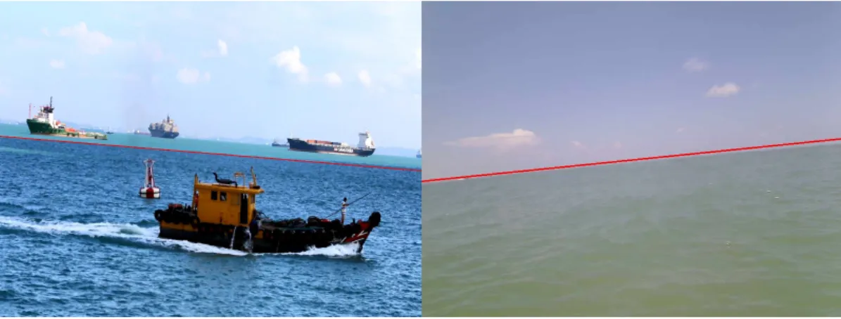
To show the validity of the described algorithm, in Figure3.4are represented two images, each one having a predicted horizon line drawn in red.

3.1 Proposed Solution 21

Figure 3.3: Representation of the exhaustive search method

Figure 3.4: Example of predicted horizon lines with region-based algorithm.

In this example, both images were down-sampled by a factor of 10. The image on the left has an original resolution of 1920 × 1080 while the image on the right has an original resolution of 800 × 600.

As can be observed, the predicted horizon is correct for the image on the right but is wrong for the image on the left. This is because the decision for choosing the optimal horizon line is made exclusively with color intensity information, ignoring other features such as textures. In doing so, as the color intensity of the sea is similar to the color intensity of the sky, the algorithm was not accurate predicting the horizon line.

In addition to not being able to make good predictions outside perfect environments, this algorithm is not also suited for a real-time implementation. A prediction of a frame with a 1920 × 1080 resolution takes 128 seconds and a prediction of a 800 × 600 frame takes 35 seconds.

With these results, the module to design would need to take into account more features other than color intensity to make its prediction and it would need to be suitable for a real-time applica-tion.

22 Methodology

Figure 3.5: Illustration of Horizonet architecture

given an input frame. Given the scope of this project, the approach was based on using a deep learning model in order to evaluate the feasibility of a machine learning solution to solve the proposed problem. An illustration of the network’s architecture is presented in figure3.5.

The network is composed by 9 convolutional layers and 2 fully connected layers.

The network takes as input an image with 416 × 416 resolution and down-samples each result-ing feature map from the convolutional layers, reachresult-ing a size of 13 × 13. The output of the 9 th convolutional layer is a feature map with a dimension of 13 × 13 × 32, which is fed into the last two layers, the fully connected layers, responsible for turning this feature map into a vector containing only two values, which represent the end points of the horizon line. The design choice of making the output of this network two discrete points instead of slope and intercept was made to ensure that the network works for every input size regardless of the frame size. Let’s consider an arbitrary horizon line in an image with a resolution of 1920 × 1080 pixels. If that same image is re-sized for a resolution of 416 × 416, the slope of the line is different, making it impossible to predict the slope of horizon line for a generic input image size, without a post-prediction transformation. We can see an example of this situation in Figures3.6and3.7.

3.2 Dataset 23

Figure 3.7: Example of an horizon detection at 416 × 416 resolution

The network also makes both horizon end-points’ predictions as a relative value to its input shape, so the transformation to the input image’s original coordinates only relies on one multipli-cation. To make sure the output is bounded between 0 and 1, it is applied the sigmoid function to the last layer of the neural network.

3.2

Dataset

To train both neural networks, it is necessary a large volume of data in order for both networks to learn how to process their inputs and make an accurate prediction. To make the training process possible, its needed a set of pictures and labels. For every picture available for training, its label needs to be available, and this label must match the network output.

3.2.1 Singapore Maritime Dataset

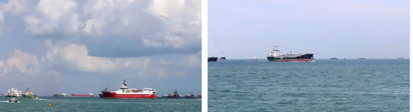
In order to meet these requirements, the Singapore Maritime Dataset (SMD) [33] was used. This dataset was captured by Dilip K. Prasad and was captured using a Canon EF 70-300mm f/4-5.6 IS USM lens on Singapore waters. All videos were acquired in high-definition, having a resolution of 1920 × 1080 pixels. The videos present in the SMD dataset were obtained on diverse environment conditions such as sunrise, mid day, sunset, haze and rain from July 2015 to May 2016.

The dataset is divided into 3 video categories:

• On-Shore, which were acquired using a camera on a fixed platform. Example in figure3.8; • On-Board, which were acquired using a camera on board of a moving vessel. Example in

figure3.9;

• Near-infra Red On-Shore, which were also acquired using a camera on a fixed platform but also it was used another Canon 70D camera with hot mirror removed and Mid-Opt BP800

24 Methodology

Figure 3.8: Sample frames from the Oh-Shore videos in the SMD.

Figure 3.9: Sample frames from the Oh-Board videos in the SMD.

3.2 Dataset 25

3.2.1.1 Classes

The Singapore Maritime Dataset contains 10 different classes of objects to classify. Those classes are present in the Table3.1.

Class Name Class Number

Ferry 1 Buoy 2 Vessel/Ship 3 Speed boat 4 Boat 5 Kayak 6 Sail boat 7 Swimming person 8 Flying bird/Plane 9 Other 10

Table 3.1: Information about the different object classes in the Singapore Maritime Dataset.

3.2.1.2 Annotations

The dataset has annotations for Object and Horizon detection. Figure3.11features a diagram of the Object ground truth data.

26 Methodology

For each frame in the video, the label contains information about all objects in that frame. Each object has information about its bounding box, represented by the pixel coordinates of its top-left corner, width and height, and the name of its class.

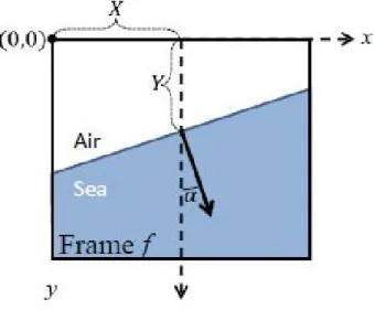
Regarding the Horizon ground truth data, its labels are composed by 4 different fields, repre-sented in figure3.12.

Figure 3.12: Diagram of Horizon Ground Truth Data

The labels contain the coordinates of the center of the horizon line - X and Y - and also contain information about the angle between the normal of the horizon line and a vertical line, namely cos(α) and sin(α).

3.2.2 Other Datasets

In addition to the Singapore Maritime Dataset, two more datasets were used, the Mar-DCT dataset [34] which is composed by videos with 800x260 pixels resolution filmed in similiar conditions as the SMD one. The other dataset used was the Buoy dataset [35], which was recorded with cameras fixed to buoys in the ocean, recording videos of 800x600 resolution.

Both datasets have the annotations in the same format as the Singapore Maritime Dataset, and the Buoy dataset only has Horizon Ground-Truth information.

3.3

Evaluation Metrics

3.3.1 IoU

Intersection over Union is a metric used to measure the accuracy of an object detector. In order to apply the IoU metric, it is necessary to have the ground truth and the predicted bounding box.

3.3 Evaluation Metrics 27

It is almost impossible to have a pixel-perfect match between a predicted and a ground-truth bounding box. Because of this difficulty, the IoU metric consists in calculating how much the predicted bounding box overlaps with the ground-truth one.

IoU = Area of Union

Area of Overlap (3.8)

With this metric, object detection algorithms have a metric that rewards predicted bounding-boxes for heavily overlapping with the groud-truth bounding-boxes.

3.3.2 Precision

The Precision metric infers how accurate the predictions actually are.

Precision= T P T P+ FPor

T P

Actual Results (3.9) where TP = True Positive and FP = False Positive.

A TP occurs when a prediction matches its ground-truth data. When a sample is miss-predicted, i.e, the prediction does not match the correct class. A FP occurs when the classifier makes a wrong prediction regarding the ground-truth data.

In the scope of this dissertation, a prediction is considered a True Positive if the bounding box has an IoU > 0.5 and the predicted class matches its ground-truth counterpart.

3.3.3 Recall

The Recall metric measures the percentage of total relevant results correctly classified.

Recall= T P T P+ FNor

T P

Predicted Results (3.10) where FN = False Negative.

A FN occurs when a ground truth sample isn’t detected.

3.3.4 mAP

The formal definition for the Average Precision is finding the area under a curve denoted as the precision-recall curve.

AP=

Z 1

0

p(r)dr (3.11)

However, some authors choose to replace the integral with a finite sum of the interpolated precision. For example, the PASCAL VOC 2007 challenge authors compute the average precision by averaging the precision over eleven evenly spaced recall levels [36].

28 Methodology

The precision is interpolated by taking the maximum precision value whose recall value is greater than r.

pinter p= max p(˜r) (3.13)

where p(˜r) is the measured precision recall ˜r ≥ r.

From 2010 onwwards, the method of computing the AP metric has changed. Instead of com-puting the interpolation over only 11 evenly spaced points, the interpolation is done over all data points. AP= 1

∑

In this case, the Average Precision is obtained by interpolating the precision at each level r taking the maximum precision whose recall value is greater or equal than r + 1 [37] [38].

Chapter 4

Experimental Setup

In this chapter, it is presented the methodology behind the training stage of both networks and how the data was selected and prepared for the training.

4.1

Environment

The system was developed with the purpose to infer the possibility and accuracy of a real-time detection system capable of operating in a maritime environment. As such, a high-end GPU is not needed to support the system.

The implementation environment was an Acer Aspire F5-573G laptop that runs on Windows 10 with an Intel(R) Core(TM) i7-6500U CPU @ 2.50GHz, NVIDIA GeForce GTX 950M GPU and 16Gb of RAM. The system was coded in Python and used the PyTorch backend for the neural network development.

The code for the YOLOv3 algorithm was adapted from [39] and [40].

4.2

Training Phase

The training stage of the proposed system is divided in two stages: train the object detector and then train the horizon detector.

Since both neural networks do not share any layers, there is no need to add a third stage to the training process to fine-tune the system by training both networks simultaneously.

4.2.1 Train and Validation

The datasets were divided into two subsets: training and validation. Since the datasets are made of videos, we chose to take every consecutive 5 frames in order to reduce multiple images of the same scenario that do not add more information capable of helping the network’s generalization abilities. This way, we can improve the speed of the training process.

30 Experimental Setup

After collecting the frames, the dataset was composed by 6964 images, with 90% destined to training and 10% to validation. It is important to note that frames belonging to the same video have to belong to the same subset in order to maintain the authenticity of the results obtained.

In Table4.1we can see the frequency of each class in each subset for the obstacle detection. Since there were videos that do not have ground truth information for both Horizon and Object detection, two separate subsets of train and validation dataset were used.

Test subset Train subset Class Name Noof Occurrences Noof Occurrences

Ferry 99 1958 Buoy 19 697 Vessel/Ship 4486 27910 Speed Boat 448 1318 Boat 132 204 Kayak 0 710 Sail Boat 0 590 Swimming Person 0 0 Flying bird/Plane 0 190 Other 1160 3947

Table 4.1: Frequency of each class within the test + train subsets

4.2.1.1 Data Augmentation

The dataset preparation also involves data augmentation in order to make the training process more robust and helping the neural network to improve its generalization of the predictions and avoiding overffiting.

The data augmentation methods used were similar to those described in the original paper [9]. It is introduced random scaling and translations up to 10% and also randomly adjustments to the color saturation and intensity by a factor of 0.5.

All bounding boxes are automatically updated with the data augmentation process, maintain-ing the authenticity of the dataset.

4.2.2 Object Detector

4.2.2.1 Training Overview

The training stage of the object detector is similar to the one described in the original paper [9]. Since the scope of this dissertation is to infer about the accuracy of an object detection algorithm in a maritime environment, the training is done using transfer learning.

The network is pre-trained in the COCO dataset, where it reached an mAP of 31.0% [11], and these weights are made available by the YOLO authors. The rationale behind using these weights to initialize the network’s parameters was to speed up the training process. Since that pre-trained network was already capable of detecting and classifying objects successfully, the main

4.2 Training Phase 31

task of the training process is to re-train the detector in order to only classify in the desired class range and retrain the last convolutional layers in order to learn the high level features associated with the desired dataset class. It is important to note that the lower convolutional layers will not be significantly affected in the training process due to the fact that they are responsible for the detection of low level features like edges or corners and those features are transversal for nearly all detectors.

With the pre-trained weights, the network is able to detect simple objects such as boats since the beginning with relative high accuracy regarding the bounding box localization. So the big focus of the training should be emphasized on classification over detection. This led to small changes on the loss function, as detailed in the next subsection.

Regarding the hyper-parameters, the training was done using a batch size of 16, learning rate of 0.001 using the stochastic gradient descent optimizer with momentum = 0.9 and weight decay = 0.0005.

4.2.2.2 Loss function

The loss function used for training the Darknet was:

Loss= λ1

∑

∑

+ λ3

_∑

_∑

where λ1, λ2, λ3and λ4are tunable parameters in order to balance the loss function. The first

two elements of the function are related to the bounding box regression, being the first one related to the center-x and center-y coordinates and the second one is related to the height and width of the bounding box. Since the pre-trained network is already accurate in locating objects, these portions of the equation will have less impact in the sum.

As the objective is to re-train the network in order for it to re-learn how to classify objects by changing the dataset, these parameters where changed versus the original paper where the original loss function was proposed [9]. As said above, the main focus of the training is in classification so, bigger emphasis was put into the third and forth elements of the loss functions, that are class confidence and object confidence respectively. To achieve the optimal values for this loss func-tion, it was applied the method of grid search, in order to obtain the best combination of these hyperparameters that result in the best network accuracy. So, the vales used for λ1, λ2, λ3and λ4,

were 8, 4, 2 and 64, respectively.

4.2.2.3 Drawbacks

The main issue regarding the training is the use of the pre-trained network, because it was trained in order to extract features necessary to locate and classify 80 different classes. In doing so, it

32 Experimental Setup

developed module. However, it is unlikely given that the scope of this system’s application is limited to a maritime environment, greatly reducing the probability of occurring such incidents.

4.2.3 Horizon Detection

4.2.3.1 Training Overview

Since the Horizon detector was developed for the purpose of this dissertation, this neural network had to be trained from scratch.

The training process is simple. The dataset is divided into train data and validation data, as described in section4.2.1. For every batch, is is computed the loss between the predicted and the ground-truth end-points of the horizon. Since the objective of the network is to have pixel-wise precision in predicting the horizon, the loss function used was the mean square error.

Losshorizonet = λ1×

_∑

Since the output of the Horizonet is normalized, it was necessary to include a parameter λ1

to ensure that the loss is correctly calculated. If this parameter did not exist, since the difference between the label and the prediction is less than 1, the mean square error of that value would be even smaller, which is not the desired behavior. For example, if the predicted output was [0.41, 0.49] and the label was [0.50, 0.54] it would produce a loss of 0.0106, which normally can be considered a good result since the loss is low. However, we have to remember that these values are scaled to the image size. If these values were to be used in an image with high resolution, for example, 1920x1080, the prediction would be [443, 529] and the label would be [540, 583]. As we can see, this difference is not negligible and this is the reason for the λ1parameter.

As hyper-parameters, the batch size is 16, the initial learning rate is 0.001 and it was selected the Adam optimizer as the network would not converge using other optimizers, like the stochastic gradient descent previously used.

As the training process is a lengthy process and can take several hours to complete even with an high-end computer with several GPUs for computing acceleration, the training was performed in the Google Colab (R) environment in order to accelerate this process. The Google Colab (R) offers free access to a Tesla T4 GPU which produces results much faster when comparing to the available hardware.

4.3

Darknet Modifications

In order to implement the Object detector, the Darknet architecture had to be updated to produce the desired output. In the last convolutional layer before each output, meaning layers 81, 93, 106, the number of output filters much match the condition f ilters = (nclasses+ 5) × 3, so the number

Chapter 5

Results

In this chapter it will be presented the results obtained for the performance of the system, correctly evaluated following the evaluation metrics previously discussed in section3.3.

5.1

Object Detector

In order to evaluate the performance of the object detector, several parameters were changed to infer its effect on the precision of the network.

5.1.1 Training Results

The Object Detector training was done during 95 epochs, with a training dataset of 5500 images and a validation dataset of 794 images. The training was done using 16 images per batch of training, resulting in a total of 32585 batches fed into the network for training, producing the results in figure5.1.

Figure 5.1: Training output

It is possible to observe that the network converged to a good output, showing that the loss associated with each element of the loss function exponentially decreased with each epoch.