Jet energy scale measurements and their systematic uncertainties in proton-proton collisions at $\sqrt{s} = 13$ TeV with the ATLAS detector

(1)

EUROPEAN ORGANISATION FOR NUCLEAR RESEARCH (CERN)

Submitted to: Phys. Rev. D. CERN-EP-2017-038

August 7, 2017

Jet energy scale measurements and their systematic

uncertainties in proton–proton collisions at

_√

s

= 13 TeV with the ATLAS detector

The ATLAS Collaboration

Jet energy scale measurements and their systematic uncertainties are reported for jets mea-sured with the ATLAS detector using proton–proton collision data with a center-of-mass en-ergy of √s= 13 TeV, corresponding to an integrated luminosity of 3.2 fb−1collected during 2015 at the LHC. Jets are reconstructed from energy deposits forming topological clusters of calorimeter cells, using the anti-kt algorithm with radius parameter R= 0.4. Jets are

cali-brated with a series of simulation-based corrections and in situ techniques. In situ techniques exploit the transverse momentum balance between a jet and a reference object such as a pho-ton, Z boson, or multijet system for jets with 20 < pT < 2000 GeV and pseudorapidities of

|η| < 4.5, using both data and simulation. An uncertainty in the jet energy scale of less than 1% is found in the central calorimeter region (|η| < 1.2) for jets with 100 < pT < 500 GeV.

An uncertainty of about 4.5% is found for low-pT jets with pT = 20 GeV in the central

re-gion, dominated by uncertainties in the corrections for multiple proton–proton interactions. The calibration of forward jets (|η| > 0.8) is derived from dijet pT balance measurements.

For jets of pT = 80 GeV, the additional uncertainty for the forward jet calibration reaches its

largest value of about 2% in the range |η| > 3.5 and in a narrow slice of 2.2 < |η| < 2.4.

c

2017 CERN for the benefit of the ATLAS Collaboration.

Reproduction of this article or parts of it is allowed as specified in the CC-BY-4.0 license.

(2)

1 Introduction

Jets are a prevalent feature of the final state in high-energy proton–proton (pp) interactions at CERN’s Large Hadron Collider (LHC). Jets, made of collimated showers of hadrons, are important elements in many Standard Model (SM) measurements and in searches for new phenomena. They are reconstructed using a clustering algorithm run on a set of input four-vectors, typically obtained from topologically associated energy deposits, charged-particle tracks, or simulated particles.

This paper details the methods used to calibrate the four-momenta of jets in Monte Carlo (MC) simulation and in data collected by the ATLAS detector [1,2] at a center-of-mass energy of √s= 13 TeV during the 2015 data-taking period of Run 2 at the LHC. The jet energy scale (JES) calibration consists of several consecutive stages derived from a combination of MC-based methods and in situ techniques. MC-based calibrations correct the reconstructed jet four-momentum to that found from the simulated stable particles within the jet. The calibrations account for features of the detector, the jet reconstruction algorithm, jet fragmentation, and the busy data-taking environment resulting from multiple pp interactions, referred to as pile-up. In situ techniques are used to measure the difference in jet response between data and MC simulation, with residual corrections applied to jets in data only. The 2015 jet calibration builds on procedures developed for the 2011 data [3] collected at √s = 7 TeV during Run 1. Aspects of the jet calibration, particularly those related to pile-up [4], were also developed on 2012 data collected at √

s= 8 TeV during Run 1.

This paper is organized as follows. Section2describes the ATLAS detector, with an emphasis on the sub-detectors relevant for jet reconstruction. Section3describes the jet reconstruction inputs and algorithms, highlighting changes in 2015. Section4describes the 2015 data set and the MC generators used in the calibration studies. Section5details the stages of the jet calibration, with particular emphasis on the 2015 in situcalibrations and their combination. Section6lists the various systematic uncertainties in the JES and describes their combination into a reduced set of nuisance parameters.

2 The ATLAS detector

The ATLAS detector consists of an inner detector tracking system spanning the pseudorapidity1 range |η| < 2.5, sampling electromagnetic and hadronic calorimeters covering the range |η| < 4.9, and a muon spectrometer spanning |η| < 2.7. A detailed description of the ATLAS experiment can be found in Ref. [1].

Charged-particle tracks are reconstructed in the inner detector (ID), which consists of three subdetectors: a silicon pixel tracker closest to the beamline, a microstrip silicon tracker, and a straw-tube transition radiation tracker farthest from the beamline. The ID is surrounded by a thin solenoid providing an axial magnetic field of 2 T, allowing the measurement of charged-particle momenta. In preparation for Run 2, a new innermost layer of the silicon pixel tracker, the insertable B-layer (IBL) [5], was introduced at a

1_{The ATLAS reference system is a Cartesian right-handed coordinate system, with the nominal collision point at the origin.} The anticlockwise beam direction defines the positive z-axis, while the positive x-axis is defined as pointing from the collision point to the center of the LHC ring and the positive y-axis points upwards. The azimuthal angle φ is measured around the beam axis, and the polar angle θ is measured with respect to the z-axis. Pseudorapidity is defined as η = − ln[tan(θ/2)], rapidity is defined as y= 0.5 ln[(E + pz)/(E − pz)], where E is the energy and pzis the z-component of the momentum, and transverse energy is defined as ET= E sin θ.

(4)

radial distance of 3.3 cm from the beamline to improve track reconstruction, pile-up mitigation, and the identification of jets initiated by b-quarks.

The ATLAS calorimeter system consists of inner electromagnetic calorimeters surrounded by hadronic calorimeters. The calorimeters are segmented in η and φ, and each region of the detector has at least three calorimeter readout layers to allow the measurement of longitudinal shower profiles. The high-granularity electromagnetic calorimeters use liquid argon (LAr) as the active material with lead absorbers in both the barrel (|η|< 1.475) and endcap (1.375 < |η| < 3.2) regions. An additional LAr presampler layer in front of the electromagnetic calorimeter within |η| < 1.8 measures the energy deposited by particles in the material upstream of the electromagnetic calorimeter. The hadronic Tile calorimeter incorporates plastic scintillator tiles and steel absorbers in the barrel (|η|< 0.8) and extended barrel (0.8 < |η| < 1.7) regions, with photomultiplier tubes (PMT) aggregating signals from a group of neighboring tiles. Scintillating tiles in the region between the barrel and the extended barrel of the Tile calorimeter serve a similar purpose to that of the presampler and were extended to increase their area of coverage during the shutdown leading up to Run 2. A LAr hadronic calorimeter with copper absorbers covers the hadronic endcap region (1.5< |η| < 3.2). A forward LAr calorimeter with copper and tungsten absorbers covers the forward calorimeter region (3.1< |η| < 4.9).

The analog signals from the LAr detectors are sampled digitally once per bunch crossing over four bunch crossings. Signals are converted to an energy measurement using an optimal digital filter, calculated from dedicated calibration runs [6,7]. The signal was previously reconstructed from five bunch crossings in Run 1, but the use of four bunch crossings was found to provide similar signal reconstruction performance with a reduced bandwidth demand. The LAr readout is sensitive to signals from the preceding 24 bunch crossings during 25 ns bunch-spacing operation in Run 2. This is in contrast to the 12 bunch-crossing sensitivity during 50 ns operation in Run 1, increasing the sensitivity to out-of-time pile-up from collisions in the preceding bunch crossings. The LAr signals are shaped [6] to reduce the measurement sensitivity to pile-up, with the shaping optimized for the busier pile-up conditions at 25 ns. In contrast, the fast readout of the Tile calorimeter [8] reduces the signal sensitivity to out-of-time pile-up from collisions in neighboring bunch crossings.

The muon spectrometer (MS) [1] surrounds the ATLAS calorimeters and measures muon tracks within |η| < 2.7 using three layers of precision tracking chambers and dedicated trigger chambers. A system of three superconducting air-core toroidal magnets provides a magnetic field for measuring muon momenta. The ATLAS trigger system begins with a hardware-based Level 1 (L1) trigger followed by a software-based high-level trigger (HLT) [9]. The L1 trigger is designed to accept events at an average 100 kHz rate, and accepted a peak rate of 70 kHz in 2015. The HLT is designed to accept events that are written out to disk at an average rate of 1 kHz and reached a peak rate of 1.4 kHz in 2015. For the trigger, jet candidates are constructed from coarse calorimeter towers using a sliding-window algorithm at L1, and are fully reconstructed in the HLT. Electrons and photons are triggered in the pseudorapidity range |η| < 2.5, where the electromagnetic calorimeter is finely segmented and track reconstruction is available. Compact electromagnetic energy deposits triggered at L1 are used as the seeds for the HLT algorithms, which are designed to identify electrons based on calorimeter and fast track reconstruction. The muon trigger at L1 is based on a coincidence of trigger chamber layers. The parameters of muon candidate tracks are then derived in the HLT by fast reconstruction algorithms in both the ID and MS. Events used in the jet calibration are selected from regions of kinematic phase space where the relevant triggers are fully efficient.

(5)

3 Jet reconstruction

The calorimeter jets used in the following studies are reconstructed at the electromagnetic energy scale (EM scale) with the anti-kt algorithm [10] and radius parameter R = 0.4 using the FastJet 2.4.3

soft-ware package [11]. A collection of three-dimensional, massless, positive-energy topological clusters (topo-clusters) [12,13] made of calorimeter cell energies are used as input to the anti-ktalgorithm.

Topo-clusters are built from neighboring calorimeter cells containing a significant energy above a noise thresh-old that is estimated from measurements of calorimeter electronic noise and simulated pile-up noise. The calorimeter cell energies are measured at the EM scale, corresponding to the energy deposited by elec-tromagnetically interacting particles. Jets are reconstructed with the anti-kt algorithm if they pass a pT

threshold of 7 GeV.

In 2015 the simulated noise levels used in the calibration of the topo-cluster reconstruction algorithm were updated using observations from Run 1 data and accounting for different data-taking conditions in 2015. This results in an increase in the simulated noise at the level of 10% with respect to the Run 1 simulation in the barrel region of the detector, and a slightly larger increase in the forward region [4]. The noise thresholds of the topo-cluster reconstruction were increased accordingly. The topo-cluster reconstruction algorithm was also improved in 2015, with topo-clusters now forbidden from being seeded by the presampler layers. This restricts jet formation from low-energy pile-up depositions that do not penetrate the calorimeters.

Jets referred to as truth jets are reconstructed using the anti-kt algorithm with R = 0.4 using stable,

final-state particles from MC generators as input. Candidate particles are required to have a lifetime of cτ > 10 mm and muons, neutrinos, and particles from pile-up activity are excluded. Truth jets are therefore defined as being measured at the particle-level energy scale. Truth jets with pT > 7 GeV and

|η| < 4.5 are used in studies of jet calibration using MC simulation. Reconstructed calorimeter jets are geometrically matched to truth jets using the distance measurement2∆R.

Tracks from charged particles used in the jet calibration are reconstructed within the full acceptance of the ID (|η| < 2.5). The track reconstruction was updated in 2015 to include the IBL and uses a neural network clustering algorithm [14], improving the separation of nearby tracks and the reconstruction performance in the high-luminosity conditions of Run 2. Reconstructed tracks are required to have a pT > 500 MeV

and to be associated with the hard-scatter vertex, defined as the primary vertex with at least two associated tracks and the largest p2_Tsum of associated tracks. Tracks must satisfy quality criteria based on the number of hits in the ID subdetectors. Tracks are assigned to jets using ghost association [15], a procedure that treats them as four-vectors of infinitesimal magnitude during the jet reconstruction and assigns them to the jet with which they are clustered.

Muon track segments are used in the jet calibration as a proxy for the uncaptured jet energy carried by energetic particles passing through the calorimeters without being fully absorbed. The segments are partial tracks constructed from hits in the MS [16] which serve as inputs to fully reconstructed tracks. Segments are assigned to jets using the method of ghost association described above for tracks, with each segment treated as an input four-vector of infinitesimal magnitude to the jet reconstruction.

2 _{The distance between two four-vectors is defined as}_{∆R = p(∆η)}2+ (∆φ)2_{, where}∆η is their distance in pseudorapidity and ∆φ is their azimuthal distance. The distance with respect to a jet is calculated from its principal axis.

(6)

4 Data and Monte Carlo simulation

Several MC generators are used to simulate pp collisions for the various jet calibration stages and for estimating systematic uncertainties in the JES. A sample of dijet events is simulated at next-to-leading-order (NLO) accuracy in perturbative QCD using Powheg-Box 2.0 [17–19]. The hard scatter is simulated with a 2 → 3 matrix element that is interfaced with the CT10 parton distribution function (PDF) set [20]. The dijet events are showered in Pythia 8.186 [21], with additional radiation simulated to the leading-logarithmic approximation through pT-ordered parton showers [22]. The simulation parameters of the

underlying event, parton showering, and hadronization are set according to the A14 event tune [23]. For in situanalyses, samples of Z bosons with jets (Z+jet) are similarly produced with Powheg+Pythia using the CT10 PDF set and the AZPHINLO event tune [24]. Samples of multijets and of photons with jets (γ+jet) are generated in Pythia, with the 2 → 2 matrix element convolved with the NNPDF2.3LO PDF set [25], and using the A14 event tune.

For studies of the systematic uncertainties, the Sherpa 2.1 [26] generator is used to simulate all relevant processes in dijet, Z+jet, and γ+jet events. Sherpa uses multileg 2 → N matrix elements that are matched to parton showers following the CKKW [27] prescription. The CT10 PDF set and default Sherpa event tune are used. The multijet systematic uncertainties are studied using the Herwig++ 2.7 [28,29] gener-ator, with the 2 → 2 matrix element convolved with the CTEQ6L1 PDF set [30]. Herwig++ simulates

additional radiation through angle-ordered parton showers, and is configured with the UE-EE-5 event tune [31].

Pile-up interactions can occur within the bunch crossing of interest (in-time) or in neighboring bunch crossings (out-of-time), altering the measured energy of a hard-scatter jet or leading to the reconstruction of additional, spurious jets. Pile-up effects are modeled using Pythia, simulated with underlying-event characteristics using the NNPDF2.3LO PDF set and A14 event tune. A number of these interactions are overlaid onto each hard-scatter event following a Poisson distribution about the mean number of additional pp collisions per bunch crossing (µ) of the event. The value of µ is proportional to the predicted instantaneous luminosity assigned to the MC event. It is simulated according to the expected distribution in the 2015 data-taking period and subsequently reweighted to the measured distribution. Events are overlaid both in-time with the simulated hard scatter and out-of-time for nearby bunches. The number of in-time and out-of-time pile-up interactions associated with an event is correlated with the number of reconstructed primary vertices (NPV) and with µ, respectively, providing a method for estimating the

per-event pile-up contribution.

Generated events are propagated through a full simulation [32] of the ATLAS detector based on Geant4 [33] which describes the interactions of the particles with the detector. Hadronic showers are simulated with the FTFP BERT model, whereas the QGSP BERT model was used in Run 1 [34]. A parameterized sim-ulation of the ATLAS calorimeter called Atlfast-II (AFII) [32] is used for faster MC production, and a dedicated MC-based calibration is derived for AFII samples.

The data set used in this study consists of 3.2 fb−1of pp collisions collected by ATLAS between August and December of 2015 with all subdetectors operational. The LHC was operated at √s = 13 TeV, with bunch crossing intervals of 25 ns. The mean number of interactions per bunch crossing was estimated through luminosity measurements [35] to be on average hµi = 13.7. The specific trigger requirements and object selections vary among the in situ analyses and are described in the relevant sections.

(7)

5 Jet energy scale calibration

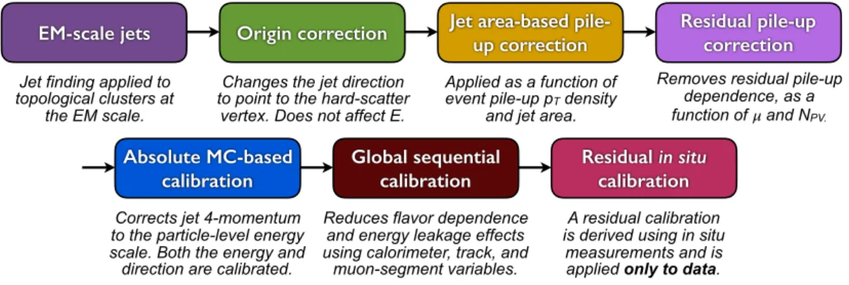
Figure1presents an overview of the 2015 ATLAS calibration scheme for EM-scale calorimeter jets. This calibration restores the jet energy scale to that of truth jets reconstructed at the particle-level energy scale. Each stage of the calibration corrects the full four-momentum unless otherwise stated, scaling the jet pT,

energy, and mass.

EM-scale jets Origin correction Jet area-based pile-_{up correction} Residual pile-up _correction

Absolute MC-based

calibration Global sequential calibration Residual in situ calibration Jet finding applied to 

topological clusters at  the EM scale.

Changes the jet direction to point to the hard-scatter

vertex. Does not affect E.

Applied as a function of event pile-up pT density

and jet area.

Removes residual pile-up dependence, as a function of 𝜇 and NPV.

Corrects jet 4-momentum  to the particle-level energy scale. Both the energy and 

direction are calibrated.

Reduces flavor dependence  and energy leakage effects using calorimeter, track, and

muon-segment variables.

A residual calibration  is derived using in situ 

measurements and is  applied only to data.

Figure 1: Calibration stages for EM-scale jets. Other than the origin correction, each stage of the calibration is applied to the four-momentum of the jet.

First, the origin correction recalculates the four-momentum of jets to point to the hard-scatter primary vertex rather than the center of the detector, while keeping the jet energy constant. This correction im-proves the η resolution of jets, as measured from the difference between reconstructed jets and truth jets in MC simulation. The η resolution improves from roughly 0.06 to 0.045 at a jet pTof 20 GeV and from

0.03 to below 0.006 above 200 GeV. The origin correction procedure in 2015 is identical to that used in the 2011 calibration [3].

Next, the pile-up correction removes the excess energy due to in-time and out-of-time pile-up. It consists of two components; an area-based pTdensity subtraction [15], applied at the per-event level, and a

resid-ual correction derived from the MC simulation, both detailed in Section5.1. The absolute JES calibration corrects the jet four-momentum to the particle-level energy scale, as derived using truth jets in dijet MC events, and is discussed in Section5.2. Further improvements to the reconstructed energy and related uncertainties are achieved through the use of calorimeter, MS, and track-based variables in the global se-quential calibration, as discussed in Section5.3. Finally, a residual in situ calibration is applied to correct jets in data using well-measured reference objects, including photons, Z bosons, and calibrated jets, as discussed in Section5.4. The full treatment and reduction of the systematic uncertainties is discussed in Section6.

5.1 Pile-up corrections

The pile-up contribution to the JES in the 2015 data-taking environment differs in several ways from Run 1. The larger center-of-mass energy affects the jet pT dependence on pile-up-sensitive variables,

while the switch from 50 to 25 ns bunch spacing increases the amount of out-of-time pile-up. In addition, the higher topo-clustering noise thresholds alter the impact of pile-up on the JES. The pile-up correction is

(8)

therefore evaluated using updated MC simulations of the 2015 detector and beam conditions. The pile-up correction in 2015 is derived using the same methods developed in 2012 [4], summarized in the following paragraphs.

First, an area-based method subtracts the per-event pile-up contribution to the pT of each jet according

to its area. The pile-up contribution is calculated from the median pT density ρ of jets in the η–φ plane.

The calculation of ρ uses only positive-energy topo-clusters with |η| < 2 that are clustered using the kt

algorithm [10, 36] with radius parameter R = 0.4. The kt algorithm is chosen for its sensitivity to soft

radiation, and is only used in the area-based method. The central |η| selection is necessitated by the higher calorimeter occupancy in the forward region. The pT density of each jet is taken to be pT/A,

where the area A of a jet is calculated using ghost association. In this procedure, simulated ghost particles of infinitesimal momentum are added uniformly in solid angle to the event before jet reconstruction. The area of a jet is then measured from the relative number of ghost particles associated with a jet after clustering. The median of the pT density is used for ρ to reduce the bias from hard-scatter jets which

populate the high-pTtails of the distribution.

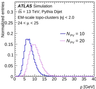
The ρ distribution of events with a given NPV is shown for MC simulation in Figure2, and has roughly

the same magnitude at 13 TeV as seen at 8 TeV. At 13 TeV the increase in the center-of-mass energy is offset by the higher noise thresholds and the larger out-of-time pile-up, the latter reducing the average energy readout of any given cell due to the inherent pile-up suppression of the bipolar shaping of LAr signals [6]. The ratio of the ρ-subtracted jet pT to the uncorrected jet pT is taken as a correction factor

applied to the jet four-momentum, and does not affect the jet η and φ coordinates.

[GeV] ρ 0 5 10 15 20 25 30 35 40 Normalized entries 0 0.05 0.1 0.15 0.2 0.25 0.3 ATLAS Simulation = 13 TeV, Pythia Dijet s | < 2.0 η EM-scale topo-clusters | < 25 µ 24 < = 10 PV N = 20 PV N

Figure 2: Per-event median pTdensity, ρ, at NPV = 10 (solid) and NPV = 20 (dotted) for 24 < µ < 25 as found in

MC simulation.

The ρ calculation is derived from the central, lower-occupancy regions of the calorimeter, and does not fully describe the pile-up sensitivity in the forward calorimeter region or in the higher-occupancy core of high-pT jets. It is therefore observed that after this correction some dependence of the anti-kt jet pT

on the amount of pile-up remains, and an additional residual correction is derived. A dependence is seen on NPV, sensitive to in-time pile-up, and µ, sensitive to out-of-time pile-up. The residual pTdependence

(9)

insensitive to pile-up. Reconstructed jets with pT > 10 GeV are geometrically matched to truth jets

within∆R = 0.3.

The residual pT dependence on NPV (α) and on µ (β) are observed to be fairly linear and independent

of one another, as was found in 2012 MC simulation. Linear fits are used to derive the initial α and β coefficients separately in bins of ptruth

T and |η|. Both the α and β coefficients are then seen to have a

logarithmic dependence on ptruth_T , and logarithmic fits are performed in the range 20 < ptruth_T < 200 GeV for each bin of |η|. In each |η| bin, the fitted value at ptruth_T = 25 GeV is taken as the nominal α and β coefficients, reflecting the dependence in the pT region where pile-up is most relevant. The logarithmic

fits over the full ptruth_T range are used for a pT-dependent systematic uncertainty in the residual pile-up

dependence. Finally, linear fits are performed to the binned coefficients as a function of |η| in 4 regions, |η| < 1.2, 1.2 < |η| < 2.2, 2.2 < |η| < 2.8, and 2.8 < |η| < 4.5. This reduces the effects of statistical fluctuations and allows the α and β coefficients to be smoothly sampled in |η|, particularly in regions of varying dependence. The pile-up-corrected pT, after the area-based and residual corrections, is given

by

pcorr_T = preco_T −ρ × A − α × (NPV− 1) − β × µ,

where preco_T refers to the EM-scale pTof the reconstructed jet before any pile-up corrections are applied.

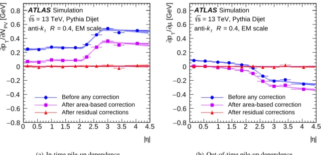
The dependence of the area-based and residual corrections on NPVand µ are shown as a function of |η| in

Figure3. The shape of the residual correction is comparable to that found in 2012 MC simulation, except in the forward region (|η| > 2.5) of Figure3(a), where it is found to be larger by 0.2 GeV. This difference

in the in-time pile-up term is primarily caused by higher topo-cluster noise thresholds, which are more consequential in the forward region.

Two in situ validation studies are performed and no statistically significant difference is observed in the jet pTdependence on NPVor µ between 2015 data and MC simulation. Four systematic uncertainties are

introduced to account for MC mismodeling of NPV, µ, and the ρ topology, as well as the pTdependence

of the NPVand µ terms used in the residual pile-up correction. The ρ topology uncertainty encapsulates

the uncertainty in the underlying event contribution to ρ through the use of several distinct MC event generators and final-state topologies. The uncertainties in the modeling of NPV and µ are taken as the

difference between MC simulation and data in the in situ validation studies. The pT-dependent uncertainty

in the residual pile-up dependence is derived from the full logarithmic fits to α and β. Both the in situ validation studies and the systematic uncertainties are described in detail in Ref. [4].

5.2 Jet energy scale andη calibration

The absolute jet energy scale and η calibration corrects the reconstructed jet four-momentum to the particle-level energy scale and accounts for biases in the jet η reconstruction. Such biases are primar-ily caused by the transition between different calorimeter technologies and sudden changes in calorimeter granularity. The calibration is derived from the Pythia MC sample using reconstructed jets after the ap-plication of the origin and pile-up corrections. The JES calibration is derived first as a correction of the reconstructed jet energy to the truth jet energy [3]. Reconstructed jets are geometrically matched to truth jets within∆R = 0.3. Only isolated jets are used, to avoid any ambiguities in the matching of calorimeter jets to truth jets. An isolated calorimeter jet is required to have no other calorimeter jet of pT > 7 GeV

(10)

| η | 0 0.5 1 1.5 2 2.5 3 3.5 4 4.5 [GeV] PV N ∂ / _T p ∂ 0.8 − 0.6 − 0.4 − 0.2 − 0 0.2 0.4 0.6 0.8 ATLAS Simulation = 13 TeV, Pythia Dijet s = 0.4, EM scale R t k

anti-Before any correction After area-based correction After residual corrections

(a) In-time pile-up dependence

| η | 0 0.5 1 1.5 2 2.5 3 3.5 4 4.5 [GeV] µ∂ / _T p ∂ 0.8 − 0.6 − 0.4 − 0.2 − 0 0.2 0.4 0.6 0.8 ATLAS Simulation = 13 TeV, Pythia Dijet s = 0.4, EM scale R t k

anti-Before any correction After area-based correction After residual corrections

(b) Out-of-time pile-up dependence

Figure 3: Dependence of EM-scale anti-ktjet pTon(a)in-time pile-up (NPVaveraged over µ) and(b)out-of-time

pile-up (µ averaged over NPV) as a function of |η| for ptruth_T = 25 GeV. The dependence is shown in bins of |η| before

pile-up corrections (blue circle), after the area-based correction (violet square), and after the residual correction (red triangle). The shaded bands represent the 68% confidence intervals of the linear fits in 4 regions of |η|. The values of the fitted dependence on in-time and out-of-time pile-up after the area-based correction (purple shaded band) are taken as the residual correction factors α and β, respectively.

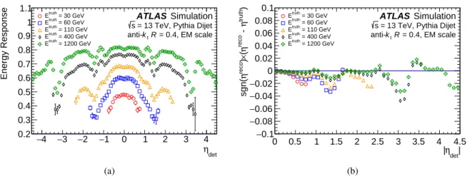
The average energy response is defined as the mean of a Gaussian fit to the core of the Ereco/Etruth distribution for jets, binned in Etruth and ηdet. The response is derived as a function of ηdet, the jet η

pointing from the geometric center of the detector, to remove any ambiguity as to which region of the detector is measuring the jet. The response in the full ATLAS simulation is shown in Figure4(a). Gaps and transitions between calorimeter subdetectors result in a lower energy response due to absorbed or undetected particles, evident when parameterized by ηdet. A numerical inversion procedure is used to

derive corrections in Erecofrom Etruth, as detailed in Ref. [13]. The average response is parameterized as a function of Erecoand the jet calibration factor is taken as the inverse of the average energy response. Good closure of the JES calibration is seen across the entire η range, compatible with that seen in the 2011 calibration. As in 2011, a small non-closure on the order of a few percent is seen for low-pTjets due

to a slightly non-Gaussian energy response and jet reconstruction threshold effects, both of which impact the response fits.

A bias is seen in the reconstructed jet η, shown in Figure4(b) as a function of |ηdet|. It is largest in jets

that encompass two calorimeter regions with different energy responses caused by changes in calorimeter geometry or technology. This artificially increases the energy of one side of the jet with respect to the other, altering the reconstructed four-momentum. The barrel–endcap (|ηdet| ∼ 1.4) and endcap–forward

(|ηdet| ∼ 3.1) transition regions can be clearly seen in Figure4(b)as susceptible to this effect. A second

correction is therefore derived as the difference between the reconstructed ηrecoand truth ηtruth, parame-terized as a function of Etruthand ηdet. A numerical inversion procedure is again used to derive corrections

in Erecofrom Etruth. Unlike the other calibration stages, the η calibration alters only the jet pTand η, not

(11)

det η 4 − −3 −2 −1 0 1 2 3 4 Energy Response 0.2 0.3 0.4 0.5 0.6 0.7 0.8 0.9 1 1.1 = 30 GeV truth E = 60 GeV truth E = 110 GeV truth E = 400 GeV truth E = 1200 GeV truth E Simulation ATLAS

= 13 TeV, Pythia Dijet s = 0.4, EM scale R t k anti-(a) | det η | 0 0.5 1 1.5 2 2.5 3 3.5 4 4.5 ) truth_η - reco η ( × ) reco_η sgn( 0.1 − 0.08 − 0.06 − 0.04 − 0.02 − 0 0.02 0.04 0.06 0.08 0.1 = 30 GeV truth E = 60 GeV truth E = 110 GeV truth E = 400 GeV truth E = 1200 GeV truth E Simulation ATLAS

= 13 TeV, Pythia Dijet s = 0.4, EM scale R t k anti-(b)

Figure 4:(a)The average energy response as a function of ηdetfor jets of a truth energy of 30, 60, 110, 400, and

1200 GeV. The energy response is shown after origin and pile-up corrections are applied.(b)The signed difference

between the truth jet ηtruthand the reconstructed jet ηrecodue to biases in the jet reconstruction. This bias is addressed with an η correction applied as a function of ηdet.

be at the EM+JES.

An absolute JES and η calibration is also derived for fast simulation samples using the same methods with a Pythia MC sample simulated with AFII. An additional JES uncertainty is introduced for AFII samples to account for a small non-closure in the calibration, particularly beyond |η| ∼ 3.2, due to the approximate treatment of hadronic showers in the forward calorimeters. This uncertainty is about 1% at a jet pT of

20 GeV and falls rapidly with increasing pT.

5.3 Global sequential calibration

Following the previous jet calibrations, residual dependencies of the JES on longitudinal and transverse features of the jet are observed. The calorimeter response and the jet reconstruction are sensitive to fluctuations in the jet particle composition and the distribution of energy within the jet. The average particle composition and shower shape of a jet varies between initiating particles, most notably between quark- and gluon-initiated jets. A quark-initiated jet will often include hadrons with a higher fraction of the jet pTthat penetrate further into the calorimeter, while a gluon-initiated jet will typically contain

more particles of softer pT, leading to a lower calorimeter response and a wider transverse profile. Five

observables are identified that improve the resolution of the JES through the global sequential calibration (GSC), a procedure explored in the 2011 calibration [13].

For each observable, an independent jet four-momentum correction is derived as a function of ptruth_T and |ηdet| by inverting the reconstructed jet response in MC events. Both the numerical inversion procedure and

the method to geometrically match reconstructed jets to truth jets are outlined in Section5.2. An overall constant is multiplied to each numerical inversion to ensure the average energy is unchanged at each stage. The effect of each correction is therefore to remove the dependence of the jet response on each observable while conserving the overall energy scale at the EM+JES. Corrections for each observable are applied independently and sequentially to the jet four-momentum, neglecting correlations between observables.

(12)

No improvement in resolution was found from including such correlations or altering the sequence of the corrections.

The five stages of the GSC account for the dependence of the jet response on (in order):

1. fTile0, the fraction of jet energy measured in the first layer of the hadronic Tile calorimeter (|ηdet|<

1.7);

2. fLAr3, the fraction of jet energy measured in the third layer of the electromagnetic LAr calorimeter

(|ηdet|< 3.5);

3. ntrk, the number of tracks with pT> 1 GeV ghost-associated with the jet (|ηdet|< 2.5);

4. Wtrk, the average pT-weighted transverse distance in the η–φ plane between the jet axis and all

tracks of pT> 1 GeV ghost-associated to the jet (|ηdet|< 2.5);

5. nsegments, the number of muon track segments ghost-associated with the jet (|ηdet|< 2.7).

The nsegments correction reduces the tails of the response distribution caused by high-pT jets that are not

fully contained in the calorimeter, referred to as punch-through jets. The first four corrections are derived as a function of jet pT, while the punch-through correction is derived as a function of jet energy, being

more correlated with the energy escaping the calorimeters.

The underlying distributions of these five observables are fairly well modeled by MC simulation. Slight differences with data have a negligible impact on the GSC as long as the dependence of the average jet response on the observables is well modeled in MC simulation. This average response dependence was tested using the dijet tag-and-probe method developed in 2011 and detailed in Section 12.1 of Ref. [13]. The average pT asymmetry between back-to-back jets was again measured in 2015 data as a function

of each observable and found to be compatible between data and MC simulation, with differences small compared to the size of the proposed corrections.

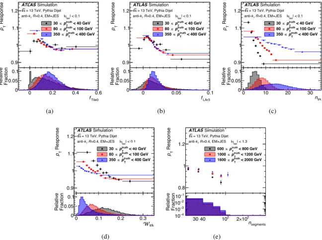
The jet pT response in MC simulation as a function of each of these observables is shown in Figure5

for several regions of ptruth_T . The distributions are shown at various stages of the GSC to reflect the relative disagreement at the stage when each correction is derived. The dependence of the jet response on each observable is reduced to less than 2% after the full GSC is applied, with small deviations from unity reflecting the correlations between observables that are unaccounted for in the corrections. The distribution of each observable in MC simulation is shown in the bottom panels in Figure5. The spike at zero in the fTile0 distribution of Figure 5(a) at low ptruth_T reflects jets that are fully contained in the

electromagnetic calorimeter and do not deposit energy in the Tile calorimeter. The negative tail in the fLAr3distribution of Figure5(b) (and, to a lesser extent, in the fTile0distribution of Figure5(a)) at low

ptruth_T reflects calorimeter noise fluctuations.

5.4 In situ calibration methods

The last stages of the jet calibration account for differences in the jet response between data and MC simulation. Such differences arise from the imperfect description of the detector response and detector material in MC simulation, as well as in the simulation of the hard scatter, underlying event, pile-up, jet formation, and electromagnetic and hadronic interactions with the detector. Differences between data and MC simulation are quantified by balancing the pT of a jet against other well-measured reference

(13)

0 0.2 0.4 0.6 Response_T p 0.9 1 1.1 1.2 < 40 GeV truth T p ≤ 30 < 100 GeV truth T p ≤ 80 < 400 GeV truth T p ≤ 350

= 13 TeV, Pythia Dijet s | < 0.1 det η =0.4, EM+JES | R t k anti-Simulation ATLAS Tile0 f 0 0.2 0.4 0.6 Fraction Relative 0 0.05 0.1 (a) 0 0.05 0.1 Response _T p 0.9 1 1.1 1.2 < 40 GeV truth T p ≤ 30 < 100 GeV truth T p ≤ 80 < 400 GeV truth T p ≤ 350

= 13 TeV, Pythia Dijet s | < 0.1 det η =0.4, EM+JES | R t k anti-Simulation ATLAS LAr3 f 0 0.05 0.1 Fraction Relative 0 0.05 0.1 (b) 0 10 20 30 Response_T p 0.9 1 1.1 1.2 < 40 GeV truth T p ≤ 30 < 100 GeV truth T p ≤ 80 < 400 GeV truth T p ≤ 350

= 13 TeV, Pythia Dijet s | < 0.1 det η =0.4, EM+JES | R t k anti-Simulation ATLAS trk n 0 10 20 30 Fraction Relative 0 0.05 0.1 (c) 0 0.1 0.2 0.3 Response_T p 0.9 1 1.1 1.2 < 40 GeV truth T p ≤ 30 < 100 GeV truth T p ≤ 80 < 400 GeV truth T p ≤ 350

= 13 TeV, Pythia Dijet s | < 0.1 det η =0.4, EM+JES | R t k anti-Simulation ATLAS trk width 0 0.1 0.2 0.3 Fraction Relative 0 0.05 0.1 (d) 30 40 ₁₀2 ₁₀2 × 2 Response_T p 0.8 1 1.2 < 800 GeV truth T p ≤ 600 < 1200 GeV truth T p ≤ 1000 < 2000 GeV truth T p ≤ 1600 = 13 TeV, Pythia Dijet s | < 1.3 det η =0.4, EM+JES | R t k anti-Simulation ATLAS segments n 30 40 ₁₀2 ₁₀2 × 2 Fraction Relative 4 − 10 3 − 10 2 − 10 1 − 10 (e)

Figure 5: The average jet response in MC simulation as a function of the GSC variables for three ranges of ptruth

T .

These include(a)the fractional energy in the first Tile calorimeter layer,(b)the fractional energy in the third LAr

calorimeter layer,(c)the number of tracks per jet,(d)the pT-weighted track width, and(e)the number of muon

track segments per jet. Jets are calibrated with the EM+JES scheme and have GSC corrections applied for the

preceding observables. The calorimeter distributions(a)and(b)are shown with no GSC corrections applied, the

track-based distributions(d)and(c)are shown with both preceding calorimeter corrections applied, and the

punch-through distribution(e)is shown with the four calorimeter and track-based corrections applied. Jets are constrained

to |η| < 0.1 for the distributions of calorimeter and track-based observables and |η| < 1.3 for the muon nsegments

distribution. The distributions of the underlying observables in MC simulation are shown in the lower panels for

each ptruth_T region, normalized to unity. The shading in the legend reflects the shading of the distributions in the

lower panel.

The η-intercalibration corrects the average response of forward jets to that of well-measured central jets using dijet events. Three other in situ calibrations correct for differences in the average response of central jets with respect to those of well-measured reference objects, each focusing on a different pTregion using

Zboson, photon, and multijet systems. For each in situ calibration the response Rin situis defined in data

and MC simulation as the average ratio of jet pTto reference object pT, binned in regions of the reference

object pT. It is proportional to the response of the calorimeter to jets at the EM+JES, but is also sensitive

to secondary effects such as gluon radiation and the loss of energy outside of the jet cone. Event selections are designed to reduce the impact of such secondary effects. Assuming that these secondary effects are

(14)

well modeled in the MC simulation, the ratio

c= R

data in situ

RMC_{in situ} (1)

is a useful estimate of the ratio of the JES in data and MC simulation. Through numerical inversion a correction is derived to the jet four-momentum. The correction is derived as a function of jet pT, and also

as a function of jet η in the η-intercalibration.

Events used in the in situ calibration analyses are required to satisfy common selection criteria. At least one reconstructed primary vertex is required with at least two associated tracks of pT > 500 MeV. Jets

are required to satisfy data-quality criteria that discriminate against calorimeter noise bursts, cosmic rays, and other non-collision backgrounds. Spurious jets from pile-up are identified and rejected through the exploitation of track-based variables by the jet vertex tagger (JVT) [4]. Jets with pT < 50 GeV and

|ηdet| < 2.4 are required to be associated with the primary vertex at the medium JVT working point,

accepting 92% of hard-scatter jets and rejecting 98% of pile-up jets.

The η-intercalibration corrects the jet energy scale of forward jets (0.8 < |ηdet| < 4.5) to that of central

jets (|ηdet| < 0.8) in a dijet system, and is discussed in Section 5.4.1. The Z/γ+jet balance analyses

use a well-calibrated photon or Z boson, the latter decaying into an electron or muon pair, to measure the pT response of the recoiling jet in the central region up to a pT of about 950 GeV, as discussed in

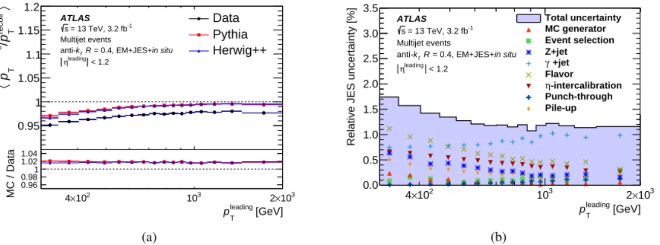
Section 5.4.2. Finally, the multijet balance (MJB) analysis calibrates central (|η| < 1.2), high-pT jets

(300 < pT < 2000 GeV) recoiling against a collection of well-calibrated, lower-pT jets, as discussed in

Section5.4.3. While the Z/γ+jet and MJB calibrations are derived from central jets, their corrections are applicable to forward jets whose energy scales have been equalized by the η-intercalibration procedure. The calibration constants derived in each of these analyses following Eq. (1) are statistically combined into a final in situ calibration covering the full kinematic region, as discussed in Section5.4.4.

The η-intercalibration, Z/γ+jet, and MJB calibrations are derived and applied sequentially, with system-atic uncertainties propagated through the chain. Systemsystem-atic uncertainties reflect three effects:

1. uncertainties arising from potential mismodeling of physics effects; 2. uncertainties in the measurement of the kinematics of the reference object; 3. uncertainties in the modeling of the pTbalance due to the selected event topology.

Systematic uncertainties arising from mismodeling of certain physics effects are estimated through the use of two distinct MC event generators. The difference between the two predictions is taken as the modeling uncertainty. Uncertainties in the kinematics of reference objects are propagated from the 1σ uncertainties in their own calibration. Uncertainties related to the event topology are addressed by varying the event selections for each in situ calibration and comparing the effect on the pT-response balance between data

and MC simulation.

Systematic uncertainty estimates depend upon data and MC samples with event yields that fluctuate when applying the systematic uncertainty variations. To obtain results that are statistically significant, the binning of Rin situin pTand η is dynamically determined for each variation using a bootstrapping

proce-dure [37]. In this procedure, pseudo-experiments are derived from the data or MC simulation by sampling each event with a weight taken from a Poisson distribution with a mean of one. Each pseudo-experiment

(15)

therefore emphasizes a unique subset of the data or MC simulation while maintaining statistical correla-tions between the nominal and varied samples. The statistical uncertainty of the response variation be-tween the nominal and varied configuration is then taken as the RMS across the pseudo-experiments, and each varied configuration is rebinned until a target significance of a few standard deviations is achieved. Bins are combined only in regions where the observed response in pTis nearly constant so that no

signif-icant features are removed.

5.4.1 η-intercalibration

In the η-intercalibration [3], well-measured jets in the central region of the detector (|ηdet|< 0.8) are used

to derive a residual calibration for jets in the forward region (0.8 < |ηdet|< 4.5). The two jets are expected

to be balanced in pTat leading order in QCD, and any imbalance can be attributed to differing responses

in the calorimeter regions, which are typically less understood in the forward region. Dijet topologies are selected in which the two leading jets are back-to-back in φ and there is no substantial contamination from a third jet. The calibration is derived from the ratio of the jet pTresponses in data and MC simulation in

bins of pTand ηdet. Two distinct NLO MC event generators are used, Powheg+Pythia and Sherpa, with

the former taken as the nominal generator. The events are generated with a 2 → 3 leading-order matrix element, increasing the accuracy of the dijet balance for events sensitive to the rejection criteria for the third jet.

The jet pTbalance is quantified by the asymmetry

A= p probe T − p ref T pavg_T ,

where pprobe_T is the transverse momentum of the forward jet, pref_T is the transverse momentum of the jet in a well-calibrated reference region, and pavg_T is the average pT of the two jets. The asymmetry is a useful

quantity as the distribution is Gaussian in fixed bins of pavg_T , whereas pprobe_T /pref_T is not. Given that the asymmetry is Gaussian, the relative jet response with respect to the reference region may be written as

*_pprobe T pref_T + ≈ 2+ hAi 2 − hAi,

where hAi is the mean value of the asymmetry distribution for a bin of pavg_T and ηdet.

Events used in the η-intercalibration follow from a combination of single-jet triggers with various pT

thresholds in regions of either |ηdet| < 3.1 or |ηdet| > 2.8. Triggers are only used in regions of kinematic

phase space in which they are 99% efficient. Triggers may also be prescaled, randomly rejecting a set fraction of events to satisfy bandwidth considerations, and the event weight is scaled proportionally. Events are required to have at least two jets with pT > 25 GeV and with |ηdet|< 4.5. Events that include a

third jet with relatively substantial pT, pjet3_T > 0.4pavg_T , are rejected. The two leading jets are also required

to be fairly back-to-back, such that∆φ > 2.5 rad.

The residual calibration is derived from the ratio of the jet responses in data and the Powheg+Pythia sample. The Sherpa sample is used to provide a systematic uncertainty in the MC modeling. The full range of |ηdet| < 4.5 is used to derive calibrations for statistically significant regions of pavg_T , offering

(16)

|ηdet| < 2.7 due to statistical considerations. A two-dimensional sliding Gaussian kernel [3] is used to

reduce statistical fluctuations while preserving the shape of the MC-to-data ratio and to extrapolate the average response into regions of low statistics.

Two η-intercalibration methods are performed that provide complementary results. In the central refer-ence method, central regions (|ηdet| < 0.8) are used as references to measure the relative jet response

in the forward probe bins (0.8 < |ηdet| < 4.5). In the matrix method, numerous independent reference

regions are chosen and the relative jet response in a given forward probe bin is measured relative to all reference regions simultaneously. The response relative to the central region is then obtained as a function of pavg_T and ηdetthrough a set of linear equations. The matrix method takes advantage of a larger data set

by allowing multiple reference regions, including forward ones, increasing the statistical precision of the calibration.

The binning is chosen such that each reference region is statistically significant in data and Powheg+Pythia samples. Some reference regions, particularly for forward probe bins, may not be statistically significant for the Sherpa sample due to its smaller sample size. Such regions are ignored in the combined fit of the response, leading to small fluctuations in the Sherpa response, which are smoothed in pTand ηdetby the

two-dimensional sliding Gaussian kernel.

The relative jet responses derived from the two methods show agreement at the level of 2%, within the uncertainty of the methods. A slightly larger response is seen in the most forward bins (|ηdet|> 2.5) in the

matrix method, as seen in 2011. This difference exists in the response in both data and MC simulation, and the MC-to-data ratio is consistent between methods. The matrix method is used to derive the nominal calibration in the following results, with the central reference method providing validation. As in the 2011 calibration, γ+jet events are also used to validate the response in the forward regions, and show good agreement between data and MC simulation in the forward region.

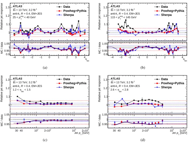
The relative jet response is shown in Figure6for both data and the two MC samples, parameterized by pT in two ηdet ranges and by ηdet in two pT ranges. The level of modeling agreement, taken between

Powheg+Pythia and Sherpa, is significantly better than in previous results and is generally within 1%, with larger differences at low pTand in forward ηdetregions. This improved agreement is not due to any

changes to the method but results from better overall particle-level agreement, particularly the improved modeling of the third-jet radiation by the NLO Powheg+Pythia and Sherpa generators over that of the LO Pythia and Herwig generators used in the 2011 calibration. The particle-level response was also measured with a Powheg-Box sample showered with Herwig++, and shows a similar level of agreement as found between Powheg+Pythia and Sherpa. Uncertainties are calculated in a given bin by shifting the observed asymmetry with all reference regions and recalculating the response. While accurate for data and Powheg+Pythia, this can lead to statistical uncertainties that do not cover the observed fluctuations in Sherpa, but that do not affect the final systematic uncertainty derived from the smoothed difference between MC samples.

The response in data is consistently larger than that in both MC samples and in the 2011 data for the forward detector region for all pT ranges. This is due to the reduction in the number of samples used to

reconstruct pulses in the LAr calorimeter from five to four, which is sensitive to differences in the pulse shape between data and MC simulation. The reduction was predicted to increase the response in the forward region, as seen in a comparison of Run 1 data processed using both five and four samples. The expected increase matches that seen in 2015 data, and is corrected for by the η-intercalibration procedure.

(17)

The effect was predicted to be particularly large for 2.3 < |ηdet|< 2.6 due to details of the jet

reconstruc-tion in calorimeter transireconstruc-tion regions. To fully account for this effect, a finer binning of ∆ηdetis used in

this region.

Relative jet response

1 1.1 1.2 1.3 ATLAS -1 = 13 TeV, 3.2 fb s = 0.4, EM+JES R t k < 40 GeV avg T p 25 < Data Powheg+Pythia Sherpa det η 4 − −3 −2 −1 0 1 2 3 4 MC / data 0.95_0.9 1 1.05 (a)

1 1.1 1.2 1.3 ATLAS -1 = 13 TeV, 3.2 fb s = 0.4, EM+JES R t k < 145 GeV avg T p 115 < Data Powheg+Pythia Sherpa det η 4 − −3 −2 −1 0 1 2 3 4 MC / data0.95_0.9 1 1.05 (b)

1 1.1 1.2 1.3 ATLAS -1 = 13 TeV, 3.2 fb s = 0.4, EM+JES R t k < 1.5 det η 1.2 < Data Powheg+Pythia Sherpa [GeV] T p Jet 30 40 ₁₀2 ₂_×₁₀2 3 10 2×103 MC / data 0.95 1 1.05 (c)

1 1.1 1.2 1.3 ATLAS -1 = 13 TeV, 3.2 fb s = 0.4, EM+JES R t k < 2.8 det η 2.6 < Data Powheg+Pythia Sherpa [GeV] T p Jet 30 40 ₁₀2 ₂_×₁₀2 3 10 2×103 MC / data 0.95 1 1.05 (d)

Figure 6: Relative response of EM+JES jets as a function of η at(a)low pTand(b)high pT, and as a function of jet

pTwithin the ranges of(c)1.2 < ηdet< 1.5 and(d)2.6 < ηdet< 2.8. The bottom panels show the MC-to-data ratios, and the overlayed curve reflects the smoothed in situ correction, appearing solid in the regions in which it is derived and dotted in the regions to which it is extrapolated by the two-dimensional sliding Gaussian kernel. Results are obtained with the matrix method. The binning is optimized for data and Powheg+Pythia, and fluctuations in the response in Sherpa are not statistically significant. Horizontal dotted lines are drawn in all at 1, 1±0.02, and 1±0.05 to guide the eye.

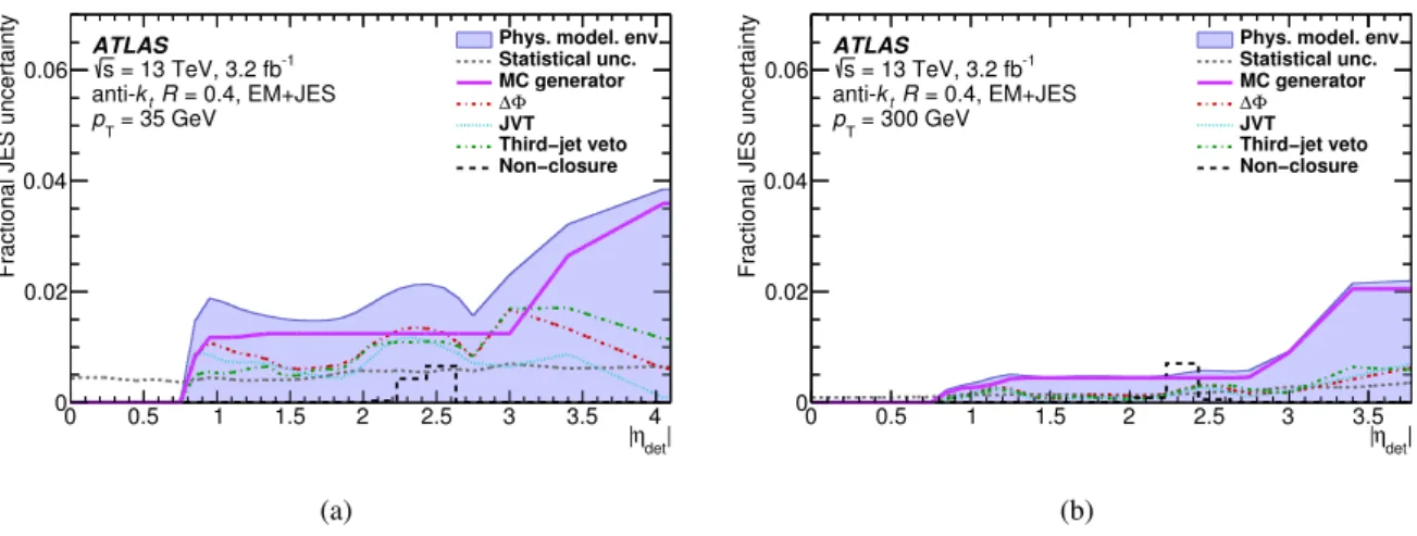
The systematic uncertainties account for physics and detector mismodelings as well as the effect of the event topology on the modeling of the pT balance. They are derived as a function of pT and |ηdet|,

with no statistically significant variations observed between positive and negative ηdet. The dominant

uncertainty due to MC mismodeling is taken as the difference in the smoothed jet response between Powheg+Pythia and Sherpa. The estimation of systematic uncertainties due to pile-up and the choice of event topology are similar to those of the 2011 calibration [3], but now use the bootstrapping procedure to ensure statistical significance. These uncertainties, including those from varying the∆φ separation requirement between the two leading jets and the third-jet veto requirement, are usually small compared to the MC uncertainty and are therefore summed in quadrature with it into a single physics mismodeling uncertainty, with a negligible loss of correlation information. Two additional and separate uncertainties

(18)

are derived to account for statistical fluctuations and the observed non-closure of the calibration for 2.0 < |ηdet| < 2.6, primarily due to the LAr pulse reconstruction effects described above. The latter is taken

as the difference between data and the nominal MC event generator after repeating the analysis with the derived calibration applied to data. The total η-intercalibration uncertainty is shown in Figure7 as a function of ηdetfor two jet pTvalues.

| det η |

0 0.5 1 1.5 2 2.5 3 3.5 4

Fractional JES uncertainty

0 0.02 0.04 0.06

Phys. model. env. Statistical unc. MC generator Φ ∆ JVT Third−jet veto Non−closure ATLAS -1 = 13 TeV, 3.2 fb s = 0.4, EM+JES R t k = 35 GeV T p (a) | det η | 0 0.5 1 1.5 2 2.5 3 3.5

Fractional JES uncertainty

0 0.02 0.04 0.06

Phys. model. env. Statistical unc. MC generator Φ ∆ JVT Third−jet veto Non−closure ATLAS -1 = 13 TeV, 3.2 fb s = 0.4, EM+JES R t k = 300 GeV T p (b)

Figure 7: Systematic uncertainties of EM+JES jets as a function of |ηdet| at (a) pT = 35 GeV and at(b) pT =

300 GeV in the η-intercalibration. The physics mismodeling envelope includes the uncertainty derived from the

alternative MC event generator as well as the uncertainties of the JVT,∆φ, and third-jet veto event selections. Also

shown are the statistical uncertainties of the MC-to-data response ratio and the localized non-closure uncertainty for 2.0 < |ηdet| < 2.6. Small fluctuations in the uncertainties are statistically significant and are smoothed in the

combination, described in Section5.4.4.

5.4.2 Z+jet and γ+jet balance

An in situ calibration of jets up to 950 GeV and with |η| < 0.8 is derived through the pT balance of a jet

against a Z boson or a photon. Z/γ+jet calibrations rely on the independent measurement and calibration of the energy of a photon or of the lepton decay products of a Z boson, through the decay channels of Z → e+e− and Z → µ+µ−. Bosons are ideal candidates for reference objects as they are precisely measured: muons from tracks in the ID and MS and photons and electrons through their relatively narrow showers in the electromagnetic calorimeter and the independent measurement of electron tracks in the ID. The Z+jet calibration is limited to the statistically significant pT range of Z boson production of

20 < pT < 500 GeV. The γ+jet calibration is limited by the small number of events at high pT and by

both dijet contamination and an artificial reduction of the number of events due to the prescaled triggers at low pT, limiting the calibration to 36 < pT< 950 GeV.

Two techniques are used to derive the response with respect to the Z boson and photon [3]. The Di-rect Balance (DB) technique measures the ratio of a fully reconstructed jet’s pT, calibrated up to the

η-intercalibration stage, and a reference object’s pT. The use of a fully reconstructed and calibrated jet

allows the calibration to be applied to jets in a straightforward manner. For a 2 → 2 Z/γ+jet event, the pT

of the jet can be expected to balance that of the reference object. However, the DB technique can be af-fected by additional parton radiation contributing to the recoil of the boson, appearing as subleading jets.

(19)

This is mitigated through a selection against events with a second jet of significant pT and a minimum

requirement on∆φ, the azimuthal angle between the Z/γ boson and the jet, to ensure they are sufficiently back-to-back in φ. The component of the boson pT perpendicular to the jet axis is also ignored, with the

reference pTdefined as

pref_T = pZ/γ_T × cos (∆φ) .

The DB technique is also affected by out-of-cone radiation, consisting of the energy lost outside of the reconstructed jet’s cone of R= 0.4 due to fragmentation processes. The out-of-cone radiation may lead to a pTimbalance between a jet and the reference boson, and is estimated by measuring the profile of tracks

around the jet axis [3].

The Missing-ET Projection Fraction (MPF) technique instead derives a pT balance between the full

hadronic recoil in an event and the reference boson. The average MPF response is defined as

RMPF = * 1+ ˆnref· ~E miss T pref_T + , (2)

where RMPFis the calorimeter response to the hadronic recoil, ˆnrefis the direction of the reference object,

and pref

T is the transverse momentum of the reference object. The ~ETmissin Eq. (2) is calculated directly

from all the topo-clusters of calorimeter cells, calibrated at the EM scale, and is corrected with the pTof

the minimum ionizing muons in Z → µµ events. No correction is needed for electrons or photons as their calorimeter response is nearly unity.

The MPF technique utilizes the full hadronic recoil of an event rather than a single reconstructed jet. The MPF response is therefore less sensitive to the jet definition, radius parameter, and out-of-cone radiation than the DB response, with reconstructed jets only explicitly used in the event selections. The MPF technique is less sensitive to the generally φ-symmetric pile-up and underlying-event activity. As the MPF technique is not derived from a reconstructed jet the correction does not directly reflect the energy within the reconstructed jet’s cone. The out-of-cone uncertainty derived for the DB technique is therefore applied as an estimate of the effect of showering and jet topology. As the MPF technique does not use jets directly, the impact of the GSC is accounted for by applying a correction to the cluster-based ~E_Tmiss, equal to the difference in momentum of the leading jet with and without the GSC. The results from this method are compared with those using no GSC and those with the GSC applied to all jets in the event, with negligible differences seen in the MC-to-data response ratio.

The response of the jet (DB) or hadronic recoil (MPF) is measured in both data and MC simulation, and a residual correction is derived using the MC-to-data ratio. The two methods are complementary and they are both pursued to check the compatibility of the measured response. The results below present the Z+jet results using the MPF technique and the γ+jet results using the DB technique.

For both techniques the average response is initially derived in bins of pref_T . In each bin of pref_T , a maximum-likelihood fit is performed using a modified Poisson distribution extended to non-integer val-ues. The fit range is limited to twice the RMS of the response distribution around the mean to minimize the effect of MC mismodeling in the tails of the distribution. The average response is taken as the mean of the best-fit Poisson distribution. For 2015 data, a new procedure is used to reparameterize the average balance from the reference object pTto the corresponding jet pT, better representing the mismeasured jet

to which the calibration is applied. This procedure is used after the calibration is derived by finding the average jet pT, without Z/γ+jet calibrations applied, within each bin of reference pT.

(20)

Events in the Z+jet selection are required to have a leading jet with pT > 10 GeV, and in the γ+jet

selection are required to have a leading jet with pT> 20 GeV. In the γ+jet DB (Z+jet MPF) technique, the

leading jet must sufficiently balance the reference boson in the azimuthal plane, requiring ∆φ(jet, Z(γ)) > 2.8 (2.9) rad. To reduce contamination from events with significant hadronic radiation, a selection of

psecond_T < max(15 GeV, 0.1 × pref_T ) is placed on the second jet, ordered by pT, in the γ+jet DB technique.

For the Z+jet MPF technique, this selection is mostly looser as RMPFis less sensitive to QCD radiation,

requiring the second jet to have psecond_T < max(12 GeV, 0.3 × pref_T ).

Electrons [38] (muons [16]) used in the Z+jet events are required to pass basic quality and isolation cuts,

and to fall within the range |η| < 2.47 (2.4). Events are selected based on the lowest-pT unprescaled

single-electron or single-muon trigger. Electrons that fall in the transition region between the barrel and the endcap of the electromagnetic calorimeter (1.37< |η| < 1.52) are rejected. Both leptons are required to have pT > 20 GeV, and the invariant mass of the opposite-charge pairs must be consistent with the

Z boson mass, with 66 < m`` < 116 GeV. Photons [38] used in the γ+jet events must satisfy tight

selection criteria and be within the range |η|< 1.37 with pT > 25 GeV. Events are selected based on a

combination of fully efficient single-photon triggers. Energy isolation criteria are applied to the photon showers to discriminate photons from π0decays and to maximize the suppression of jets misidentified as photons [39]. Jets within∆R = 0.35 of a lepton are removed from consideration in the Z+jet selection, while jets within∆R = 0.2 of photons are similarly removed from consideration in both the Z+jet and γ+jet selections.

The average response in Z/γ+jet events as a function of jet pT is shown in Figure 8for data and two

MC samples. For the DB technique in γ+jet events, the response is slightly below unity, reflecting the fraction of pTfalling outside of the reconstructed jet cone. For the MPF technique in Z+jet events, RMPF

is significantly below unity, reflecting that the Z boson is fully calibrated while the topo-clusters used in calculating the hadronic recoil are at the EM scale. However, in both cases the data and MC simulation are in agreement, with the MC-to-data ratio within ∼5% of unity for both MC samples. The rise in RMPF

at low pTin Figure8(a)is caused by the jet reconstruction threshold.

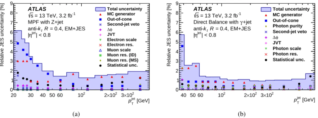
Systematic uncertainties in the MC-to-data response ratios are shown in Figure9. In both the DB and MPF techniques the event selections are varied to estimate the impact of the choice of event topology on the MC mismodeling of the pTresponse. Variations are made to the selection criteria for the second-jet pTand∆φ

between the leading jet and reference object to assess the effect of additional parton radiation. The effect of pile-up suppression is similarly studied by varying the JVT cut about its nominal value. Potential MC event generator mismodeling is explored by repeating the analyses with alternative MC event generators, with the difference in the MC-to-data response ratios taken as a systematic uncertainty. Uncertainties in the energy (momentum) scale and resolution of electrons and photons (muons) are estimated from studies of Z → ee (Z → µµ) measurements in data [16,38]. Variations of ±1σ are propagated through the analyses to the MC-to-data response ratios. A purity uncertainty in the γ+jet balance accounts for the contamination from multijet events arising from jets appearing as fake photons. The effect of this contamination on the MC-to-data response ratio is studied by relaxing the photon identification criteria. The uncertainty due to out-of-cone radiation is derived from differences between data and MC simulation in the transverse momentum of charged-particle tracks around the jet axis. The bootstrapping procedure is used to ensure only statistically significant variations of the response are included in the uncertainties.

(21)

20 30 40 50 60 102 2×102 3×102 MPF R 0.4 0.5 0.6 0.7 0.8 0.9 1.0 1.1 Data Powheg+Pythia Sherpa ATLAS -1 = 13 TeV, 3.2 fb s MPF with Z+jet = 0.4, EM+JES R t k anti-| < 0.8 jet η | [GeV] jet T p 20 30 40 50 102 2×102 MC / Data 0.9 1.0 1.1 (a) [GeV] jet T p 40 50 ₁₀2 ₂_×₁₀2 〉 ref T p/ jet T p 〈 0.85 0.9 0.95 1 1.05 1.1 1.15 1.2 Data Pythia Sherpa ATLAS -1 = 13 TeV, 3.2 fb s +jet γ

Direct Balance with = 0.4, EM+JES R t k anti-| < 0.8 jet η | [GeV] jet T p 40 50 ₁₀2 ₂_×₁₀2 MC / Data 0.95 1 1.05 1.1 (b)

Figure 8: The average(a)MPF response in Z+jet events and(b)Direct Balance jet pTresponse in γ+jet events as

a function of jet pTfor EM+JES jets calibrated up to the η-intercalibration. The response is given for data and two

distinct MC samples, and the MC-to-data ratio plots in the bottom panels reflect the derived in situ corrections. A dotted line is drawn at unity in the top-right panel and bottom panels to guide the eye.

[GeV]

jet T

p

20 30 40 50 60 ₁₀2 ₂_×₁₀2 ₃_×₁₀2

Relative JES uncertainty [%]

0 1 2 3 4 5 6 7 8 9 Total uncertainty MC generator Out-of-cone Second-jet veto φ ∆ JVT Electron scale Electron res. Muon scale Muon res. (ID) Muon res. (MS) Statistical unc. ATLAS -1 = 13 TeV, 3.2 fb s MPF with Z+jet = 0.4, EM+JES R t k anti-| < 0.8 jet η | (a) [GeV] jet T p 40 50 60 ₁₀2 ₂_×₁₀2 ₃_×₁₀2

Relative JES uncertainty [%]

0 1 2 3 4 5 6 7 8 9 Total uncertainty MC generator Out-of-cone Photon purity Second-jet veto φ ∆ JVT Photon scale Photon res. Statistical unc. ATLAS -1 = 13 TeV, 3.2 fb s +jet γ

Direct Balance with = 0.4, EM+JES R t k anti-| < 0.8 jet η | (b)

Figure 9: Systematic uncertainties of EM+JES jets, calibrated up to the η-intercalibration, as a function of jet pT

for(a)Z+jet events using the MPF technique and(b)γ+jet events using the Direct Balance technique. Uncertainties

account for out-of-cone radiation and variations of the JVT,∆φ, second-jet veto, and photon purity event selections.

Uncertainties are also propagated from the electron and photon energy scale and resolution and the muon momen-tum scale and resolution in the ID and MS. Also shown are the statistical uncertainties of the MC-to-data response ratio and the uncertainty derived from an alternative MC event generator. Small fluctuations in the uncertainties are