UNIVERSIDADE DE LISBOA
FACULDADE DE CIÊNCIAS
DEPARTAMENTO DE FÍSICA
Prostate Cancer Biochemical Recurrence Prediction After
Radical Prostatectomy Using Machine Learning Analysis of
Histopathology
Carolina Alexandra Carrapiço Seabra
Mestrado Integrado em Engenharia Biomédica e Biofísica
Perfil em Radiações em Diagnóstico e Terapia
Dissertação orientada por:
Dra. Raquel Conceição
Dr. Nickolas Papanikolaou
First of all, I would to thank Doctor Nickolas Papanikolaou, for taking me in the Compu-tational Clinical Imaging group at the Champalimaud Foundation. I am thankful to be part of such an important research institution and experience a truly clinical research environment.
My deepest appreciation is extended to Professor Raquel Cruz Concei¸c˜ao. I am grateful for all her support, regular and prompt feedback, motivation, guidance and optimism throughout all the project. I am thankful for her aspiring guidance, invaluably constructive criticism and friendly advice. Apart from her supervisor role, Professor Raquel was also a friend who kindly dealt with my ”struggle” and cheered me up to continue this work. She is an inspiration for me, not only because of her ability to show her passion for the work she does, her immense knowledge and dedication to everything she is involved in, but mainly because of her kind, caring and assertive personality. It is my deepest belief, I would not have reach far without her. Special mention goes to Prof Dr Doctor Ant´onio Beltran, without whom I would still be trying to learn how to differentiate between positive and negative images. Although we spent a lot of the time doing a laborious task as checking thousands of images to perform the annotations, Prof. Dr. Ant´onio was always in a good mood, especially when ”PIN’s guapos” came into view. It was such an opportunity for me to work in this project with him. The longer I spent with him, the more impressed I felt with his expertise, excitement and professionalism.
I would also like to express my gratitude to the rest of the group, especially Jo˜ao Santinha. He was always willing to generously share his time, providing me invaluable help with com-puter/programming issues. Our discussions over my problems and findings allowed me to choose the right direction and successfully complete my dissertation. A big thanks is also extended to Jos´e Moreia for all his help and support regarding deep learning and NiftyNet issues. Without his immense expertise I would have not been able to successfully develop my models. A special mention goes to author of the ”Parallel Genetic Algorithms For Financial Pattern Discovery Using Gpus” bestseller. Jo˜ao Ba´uto saved me from loosing all my data a couple of times and played a decisive role, as far as the training of my models are concerned. The long hours he was willing to spent with me waiting for results were everything but boring. His intelligence, willingness to help others, sense of humor, kindness make him one of the most amazing persons I had the pleasure to meet, during the last year.
This journey would not have been the same without my dearest friend M´onica. Thank you for support, laughter, patience, silliness, encouragement, conversations, hugs, cookies... Sara for your happy mood and all the end of day skate rides. Neusa, Laeticia and Hon´orio, I am very thankful to have you as my friends and this journey would not be the same without your friendliness. Last but not least important, I owe more than thanks to my family, for their support and encouragement throughout my life. My mother who gives me unconditional support and guides me through the difficult situations. All that I am or hope to be I owe to you.
O cancro de pr´ostata ´e o segundo tipo de cancro com maior prevalˆencia nos homens, em todo o mundo. A dete¸c˜ao inicial desta doen¸ca ocorre, geralmente, durante exames e consultas de rotina, quando n´ıveis aumentados do antig´enio prost´atico espec´ıfico e/ou um exame retal anormal s˜ao descobertos. Contudo, apenas a avalia¸c˜ao histopatol´ogica, inicialmente baseada em amostras extra´ıdas atrav´es de uma bi´opsia, ´e capaz de fornecer um diagn´ostico definitivo, permitindo n˜ao s´o orientar o tratamento do doente, assim como o processo de tomada de decis˜ao associado. Ap´os esta avalia¸c˜ao inicial, se o doente for diagnosticado com cancro da pr´ostata localizado, ou seja, um tumor confinado `a pr´ostata, o tratamento mais adotado ´e a prostatectomia radical. Este ´ultimo ´e o tratamento padr˜ao utilizado quando se pretende uma terapia com curativa. A vantagem da t´ecnica de prostatectomia radical ´e que, toda a pr´ostata, onde o tumor se encontra confinado, ´e removida cirurgicamente, auxiliando na redu¸c˜ao do risco de met´astases.
A posterior an´alise da pe¸ca prost´atica permite ao patologista avaliar diversas caracter´ısticas tumorais, determinantes no progn´ostico do doente. Para este fim, o microsc´opio tem sido a prin-cipal ferramenta utilizada, uma vez que proporciona imagens ao vivo com uma ´otima resolu¸c˜ao. No entanto, desde a introdu¸c˜ao do primeiro sistema automatizado de digitaliza¸c˜ao de lˆaminas em imagens de alta resolu¸c˜ao, o interesse da comunidade de anatomia patol´ogica em explorar este tipo de m´etodos para diferentes aplica¸c˜oes tem crescido exponencialmente. O potencial desta nova ´area n˜ao ´e, todavia, a simples transferˆencia de uma imagem da lˆamina de vidro para um monitor, nem t˜ao pouco a flexibilidade de distribui¸c˜ao e modifica¸c˜ao da pr´opria imagem digital, mas sim, a possibilidade de aprimorar a avalia¸c˜ao do patologista com informa¸c˜oes e inteligˆencia que n˜ao podem ser detetados pela an´alise humana.
Por conseguinte, a implementa¸c˜ao de algoritmos de aprendizagem autom´atica capazes de executar tarefas como dete¸c˜ao, classifica¸c˜ao e segmenta¸c˜ao de imagens digitais histopatol´ogicas ´e, finalmente, poss´ıvel. Estes m´etodos de an´alise automatizada permitem explorar todo o panorama morfol´ogico do tumor e dos seus elementos mais invasivos presentes, capturando, por exemplo, a orienta¸c˜ao nuclear, a textura, a forma e a arquitetura. A complexidade e densidade inerente a este tipo de imagens, oferecem uma abundˆancia de informa¸c˜ao, ideal para estimular e promover o desenvolvimento de algoritmos baseados em deep learning. No que diz respeito ao cancro da pr´ostata, os algoritmos desenvolvidos visam apoiar as avalia¸c˜oes efetuados pelos patologistas, nomeadamente, estadiamento e classifica¸c˜ao, sendo, portanto, focados no sistema de classifica¸c˜ao utilizada para a pr´ostata - o Gleason score. Contudo, problem´aticas alternativas podem tamb´em beneficiar da aplica¸c˜ao destas t´ecnicas, nomeadamente m´etodos capazes de distinguir imagens que apenas contˆem tecido benigno de imagens em que tumor esteja presente. Por outro lado, modelos capazes de prever a recidiva bioqu´ımica de cancro da pr´ostata permitiriam aos m´edicos modificar estrat´egias de tratamento e p´os-tratamento, a fim de equilibrar benef´ıcios e efeitos adversos de um terapia espec´ıfica. A previs˜ao de recidiva permite, tamb´em, que os pacientes
Desta forma, com o objetivo de explorar os referidos problemas, a presente disserta¸c˜ao apre-senta procedimentos de recolha, processamento e anota¸c˜ao de dados, que permitiram a cria¸c˜ao de uma base digital de dados histol´ogicos anotados da pr´ostata. Com base nestes dados dois modelos distintos de deep learning, especificamente Convolutional Neural Networks foram desen-volvidos. O modelo I prop˜oe a identifica¸c˜ao de cancro da pr´ostata e diferencia¸c˜ao entre tumor e tecido benigno. O modelo II pretende prever a condi¸c˜ao de recidiva bioqu´ımica do cancro de pr´ostata, para um per´ıodo de tempo posterior `a cirurgia em dois anos.
Relativamente ao desenvolvimento da base de dados, 200 casos de cancro da pr´ostata, trata-dos atrav´es de prostatectomia radical, foram selecionados. As lˆaminas correspondentes `a les˜ao ´ındice, ou seja, `a les˜ao principal, foram identificadas e, apenas estas foram inclu´ıdas na amostra final. A ado¸c˜ao desta abordagem deveu-se ao facto de que cada pe¸ca origina entre 15-45 lˆaminas, sendo que a maioria n˜ao cont´em tumor. Por outro lado, dado o per´ıodo de tempo para a real-iza¸c˜ao de todo este projeto, seria invi´avel a utiliza¸c˜ao de todas as lˆaminas. Assim, as lˆaminas selecionadas foram digitalizadas e processadas. Uma t´ecnica de normaliza¸c˜ao de contraste foi aplicada, de forma a uniformizar as cores das diferentes imagens digitais, evitando uma elevada variabilidade de contraste e cor que adv´em da utiliza¸c˜ao de diferentes protocolos de cor, bem como da pr´opria digitaliza¸c˜ao da lˆamina. As imagens histol´ogicas digitalizadas e normalizadas foram posteriormente divididas em imagens mais pequenas, isto ´e, subimagens, uma vez que desta forma existe uma otimiza¸c˜ao da extra¸c˜ao de caracter´ısticas por parte dos algoritmos. Es-tas subimagens foram individualmente visualizadas e anotadas, originando um total de cerca de 160,000 subimagens, correspondentes aos 200 casos diferentes selecionados.
Para o desenvolvimento do modelo de classifica¸c˜ao do cancro de pr´ostata, a arquitetura Inception v3 foi implementada e treinada utilizando as subimagens da base de dados. Este modelo foi capaz de identificar trˆes classes distintas: negativa (tecido benigno), positiva (tecido maligno) e neoplasia intraepitelial da pr´ostata, esta ´ultima, embora com menor precis˜ao dada a quantidade reduzida de exemplos pertencentes a esta classe. Um valor de 93 % de precis˜ao foi obtido, o que corresponde a valores equiparados ao estado da arte para este tipo de t´ecnicas. Este valor, contudo, demonstra ainda potencial para otimiza¸c˜ao e melhoria, uma vez que as diferentes classes dos dados utilizados seguiam uma distribui¸c˜ao n˜ao equilibrada. A inclus˜ao de mais casos cl´ınicos e a aplica¸c˜ao de t´ecnicas de aumento de dados, podem ser facilmente realizadas, o que culminar´a num modelo com ainda melhor precis˜ao de classifica¸c˜ao.
Relativamente ao modelo referente `a previs˜ao de recidiva bioqu´ımica, a mesma arquitetura foi utilizada, mas neste caso, treinada apenas com base nas subimagens positivas, isto ´e, as subim-agens contendo tecido maligno da pr´ostata. Os resultados obtidos revelaram que este modelo n˜ao tem a capacidade de extrair informa¸c˜ao relevante correlacionada com o objetivo do estudo, e portanto, n˜ao consegue distinguir com sucesso casos n˜ao recorrentes de casos recorrentes, pro-duzindo apenas uma precis˜ao de 60 %. Contudo, apesar do referido modelo falhar na execu¸c˜ao do objetivo estipulado, ´e fundamental notar que a tarefa de predi¸c˜ao de recidiva bioqu´ımica ´e de complexidade elevada, n˜ao sendo poss´ıvel aos patologistas, atrav´es da observa¸c˜ao das ima-gens histol´ogicas, retirar nenhuma conclus˜ao que diretamente se correlacione com esta condi¸c˜ao. Diferentes abordagens, como por exemplo, o aumento da quantidade de dados utilizados, a introdu¸c˜ao no modelo de caracter´ısticas cl´ınicas relevantes no progn´ostico da doen¸ca poder˜ao apresentar melhorias substanciais, no que diz respeito `a capacidade preditiva deste modelo.
O desenvolvimento e o cria¸c˜ao de uma base de dados anotados, fornece a base fundamental para o desenvolvimento de modelos adicionais, onde diversas quest˜oes podem ser exploradas. O desenvolvimento de uma interface que permita implementar o modelo de dete¸c˜ao de cancro da pr´ostata desenvolvido ´e tamb´em uma possibilidade, uma vez que fornece eficiˆencia e consistˆencia, beneficiando a pr´atica da patologia clinica.
Palavras-Chave: Cancro da Pr´ostata; Recidiva Bioqu´ımica; Patologia Digital; Deep Learn-ing.
Prostate cancer is the second most prevalent cancer in men, worldwide. Histopathologi-cal assessment plays an indispensable role in understanding the disease mechanisms, providing definitive diagnosis to guide patient treatment and management decisions. The microscope has been the primary tool to this end, producing images at increased resolution. However, with the development of the first automated high resolution whole-slide imaging system, which allows the digitisation of glass slides, interest in using this system for different applications in pathology practice has steadily grown, giving rise to the digital pathology field. The promise of digital pathology is not, however, the simple transfer of an image from a glass slide to a monitor, not even the flexibility of distribution and modification of the image, but instead the potential to enhance the pathologist’s assessment with information and artificial intelligence that cannot be perceived by human examination.
With the advent of digital pathology and the recent expert-level accuracy achieved by ma-chine learning based algorithms in medical image detection, classification and segmentation, new possibilities to develop automated image analysis methods arise. As far as prostate can-cer is concan-cerned, these models have been aimed at supporting pathologist’s image descriptions such as staging and grading, being hence, focused on the Gleason grading system. In order to explore alternative problems, the present dissertation presents data collection, processing and annotation procedures, that allowed the creation of an annotated digital histology database of prostate resection cases. These data was used to develop deep learning models not only to clas-sify prostate cancer, but also to predict prostate cancer biochemical recurrence. Inception v3 architecture was implemented and trained from scratch for the proposed assignments.
The prostate cancer classification model yielded an accuracy of 93%, being able to iden-tify three distinct classes: negative (benign tissue), positive (malignant tissue) and high-grade prostate intraepithelium neoplasia, the latter, although, with lower precision, given to unbal-anced class distributions. The prostate cancer biochemical prediction model was not able to successfully distinguish between non-recurrent and recurrent cases, yielding an accuracy of 60%. This value was accomplished, nevertheless, due to the fact that the model was classifying all en-tries as negative, and therefore, the value of accuracy corresponds to the percentage of negative cases present in the dataset.
Although not all models here developed achieved good results, the capacity of deep learning algorithms to harvest relevant features from prostate histopathology digital images has been demonstrated. The development and establishment of an annotated database provides the fun-damental basis to further develop additional models, and mainly to improve the biochemical recurrence prediction model by applying more sophisticated methods, given the complexity of this problem.
List of Figures xi
List of Tables xiii
List of Abbreviations xv
1 INTRODUCTION 1
1.1 Context and Motivation . . . 1
1.2 Objectives . . . 2
1.3 Outline . . . 2
2 LITERATURE REVIEW 3 2.1 Prostate Gland . . . 3
2.1.1 Prostate Anatomy and Histology . . . 3
2.1.2 Prostate Cancer . . . 5
2.1.2.1 Prostate Cancer Diagnosis . . . 5
2.1.2.2 Pathology of the Prostate Cancer . . . 6
2.1.2.3 Prostate Cancer Treatment . . . 9
2.1.3 Prostate Cancer Biochemical Recurrence Prediction . . . 11
2.2 Anatomic Pathology . . . 12
2.2.1 Fundamentals of Anatomic Pathology . . . 12
2.2.2 Digital Pathology . . . 13
2.2.2.1 Intelligent Digital Pathology . . . . 14
2.3 Deep Learning . . . 16
2.3.1 Basic Concepts of Neural Networks . . . 16
2.3.2 Training a Neural Network . . . 18
2.3.2.1 Hyperparameters Tuning . . . 19
2.3.2.2 Datasets, Overfitting and Regularisation . . . 20
2.3.3 Evaluation Metrics . . . 21
2.3.4 Convolutional Neural Networks (CNN) . . . 22
3 MATERIALS AND METHODS 25 3.1 Data Description . . . 25
3.2 Data Collection . . . 25
3.3 Whole Slide Image Processing . . . 26
3.3.1 Colour Normalisation . . . 26
3.3.3 Annotations . . . 27
3.4 Deep Learning and CNN . . . 28
3.4.1 Inception V3 Implementation . . . 28
3.4.2 Model I: PCa Classification . . . 29
3.4.3 Model II: PCa Biochemical Recurrence Prediction . . . 30
4 RESULTS 33 4.1 Importance of Image Processing . . . 33
4.2 Model I: PCa Classification . . . 35
4.2.1 Non-normalised images . . . 36
4.2.2 Normalised images . . . 38
4.3 Model II: PCa Biochemical Recurrence Prediction . . . 40
4.3.1 Resampling of the Original Dataset . . . 43
5 DISCUSSION 45 6 CONCLUSIONS 51 References 53 Appendix 61 A.1 Ethics Committee Submission Documents . . . 61
2.1 Sagittal section of the male pelvis. . . 3
2.2 Zonal anatomy of the normal prostate as described by McNeal. . . 4
2.3 Lesions and structures that can simulate prostate cancer. . . 6
2.4 BPH foci in low and high magnification. . . 7
2.5 Low magnification of different patterns of atrophy. . . 8
2.6 Atrophic prostate carcinoma may be occasionally cystic and resembling a focus of benign atrophy. . . 8
2.7 High power view of the different PIN categories: low grade and high-grade. . . . 9
2.8 Example of carcinoma of the prostate, which resembles a PIN foci. . . 9
2.9 Schematic illustration of architectural patterns of high-grade PIN. . . 10
2.10 Diagram representing the histology process which allows a diagnosis to be rendered. 12 2.11 Pyramid structure representing the various resolutions that compose a whole slide image. . . 14
2.12 Digital pathology workstation. . . 15
2.13 Architecture of simple neural network. . . 17
2.14 Schematic representation of an artificial neuron. . . 18
2.15 Confusion matrix for a binary classifier. . . 21
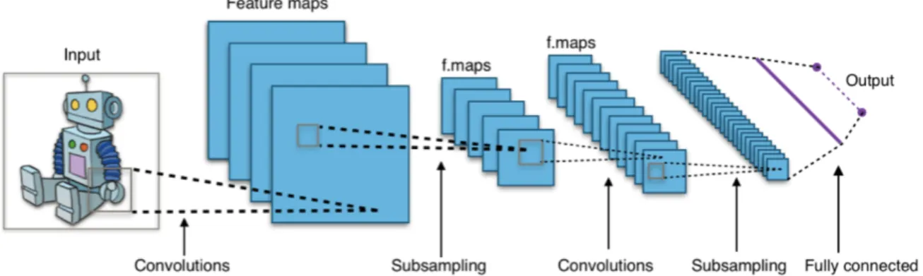
2.16 Basic CNN architecture composed of convolutional layers, followed by subsam-pling and fully connected layers. . . 22
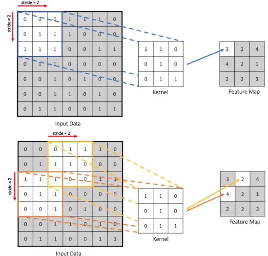
2.17 Schematic representation of the convolution process. . . 23
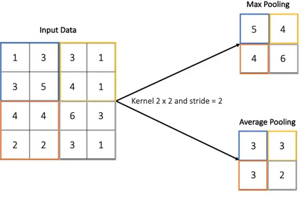
2.18 Schematic illustration of the pooling process. . . 24
3.1 Completed phases needed to transform the glass slide images into digital format. 26 3.2 Overview of a k-fold cross-validation example. . . 32
4.1 Illustration of the performance of the colour normalisation technique. . . 34
4.2 Schematic representation of the performed patching approach. . . 34
4.3 Distinguished classes during the annotation process. . . 35
4.4 Accuracy progression for model I with non-normalised images. . . 36
4.5 Loss progression for model I with non-normalised images. . . 37
4.6 Normalised testset confusion matrix, corresponding to the results of model I for non-normalised images. . . 37
4.7 Accuracy progression for model I with normalised images. . . 39
4.8 Loss progression for model I with normalised images. . . 39
4.9 Normalised testset confusion matrix, corresponding to the results of model I for normalised images. . . 40
4.10 Accuracy progression for model II. . . 41
4.11 Loss progression for model II. . . 42
4.12 Testset confusion matrix, corresponding to the results of model II. . . 42
4.13 Accuracy progression for model II with the resampled dataset. . . 43
3.1 Number of cases, slides and generated patches for the two models developed in
this study. . . 28
3.2 Hardware and Software specifications of the compute machine. . . 29
3.3 Class representation for the dataset used to develop model I. . . 29
3.4 Class representation for the dataset used to develop model II. . . 31
4.1 Learning parameters used to develop model I, both for non-normalised and nor-malised images. . . 35
4.2 Evaluation metrics calculated for 5 folds during the training/validation phase, concerning non-normalised images. The highlighted row corresponds to the fold yielding the best performance model. . . 36
4.3 Final values of accuracy and Cohen’s Kappa coefficient yielded by the non-normalised images test dataset. . . 38
4.4 Different evaluation metrics calculated for the non-normalised images test dataset. 38 4.5 Evaluation metrics calculated for 5 folds during the training/validation phase, concerning normalised images. The highlighted row corresponds to the fold yield-ing the best performance model. . . 38
4.6 Accuracy and Cohen’s Kappa Coefficient evaluation metrics for the testset, con-cerning normalised images. . . 40
4.7 Different evaluation metrics calculated for the normalised images test dataset. . . 40
4.8 Learning parameters used to develop model II. . . 41
4.9 Accuracy and Cohen’s Kappa coefficient evaluation metrics calculated for the training/validation phase of model II. . . 41
4.10 Different evaluation metrics calculated for the model II test dataset. . . 43
ANN . . . Artificial Neural Networks AUC . . . Area Under the Curve BCR . . . Biochemical Recurrence BPH . . . Benign Prostatic Hyperplasia CAD . . . Computer Aided Diagnosis CNN . . . Convolutional Neural Networks CT . . . Computed Tomography
DRE . . . Digital Rectal Examination FDA . . . Food and Drug Administration H&E . . . Hematoxylin and Eosin
MRI . . . Magnetic Resonance Imaging PCa . . . Prostate Cancer
PIN . . . Prostate Intraepithelium Neoplasia PSA . . . Prostate Specific Antigen
ReLU . . . Rectified Linear Unit RGB . . . Red Green Blue
SGD . . . Stochastic Gradient Descent
SPCN . . . Structure Preserving Color Normalization SVI . . . Seminal Vesicle Involvement
TCGA . . . The Cancer Genome Atlas TRUS . . . TransRectal Ultrasound WHO . . . World Health Organization WSI . . . Whole Slide Imaging
1
INTRODUCTION
In this dissertation an approach to classification of prostate cancer and prediction of relapse is presented. The first chapter not only offers a brief contextualisation of why prostate cancer is a health issue, but also presents the goals of the project. Finally, the dissertation outline is also also described.
1.1
Context and Motivation
Men who are diagnosed with prostate cancer, and the physicians who care for them are faced with a wealth of information about this disease, including a variety of treatment options. While some cancers lay dormant for many years, others progress rapidly, being therefore, risk assessment a critical step in disease management, determining whether the cancer can simply be monitored, or a radical intervention by prostatectomy is needed. Among the involved procedures, the most important one is the examination of the biopsy and/or surgical tissue specimen by a pathologist. The image analysis of these prostate histopathological samples is used to provide the final detailed diagnosis and prognosis.
Current histopathology practice has several constraints, as it is highly time-consuming and it is often prone to inconsistencies and low agreement between pathologists. The staging and grading of prostate cancer is getting increasingly complex due to cancer incidence and patient-specific treatment options. The detailed analysis of a single case could require several slides with multiple stainings. Moreover, quantitative parameters are increasingly required (such as mitoses counting), increasing the pressure on pathologists to handle large volumes of cases, while still providing large amounts of information in the pathology reports. In this sense, the interest in digital pathology has continuously grown.
A high resolution automated system of whole slide imaging has been a strong advance for pathology, overcoming limitations, such as poor image quality and image navigation. It com-plements optical microscopies, also allowing for the application of visualisation software. This evolution can lead to virtual storage of images of pathological anatomy, and the associated es-tablishment of global databases of histopathology images, which could be used both for clinical and educational purposes. On the other hand, it provides the opportunity to share clinical cases among health professionals, a key to clinical efficiency, given that the temporal window in which the diagnosis takes place is crucial for the hope of survival of many patients.
Nevertheless, the advantages of digital pathology are not yet sufficiently explored. There is a need to develop tools for automated tissue images processing and automated algorithm analysis
which can positively aid pathologists in decision making and improve the diagnosis/prognosis output. Recently, deep convolutional neural networks have revolutionised many medical image analysis domains, one of them being histopathology image grading and classification. Further exploration of deep learning approaches to histopathology tasks will certainly reveal its tremen-dous potential. Therefore, in this dissertation an approach to classification of prostate cancer and prediction of relapse is presented.
1.2
Objectives
The overall aim of the present work was to evaluate the power of machine learning based algorithms by developing and evaluating new classification and prognostic models based on histological digital images of the prostate. The secondary goals included:
(i) Comprehension of the main issues in classification and prediction tasks of pathology slides. (ii) Analysis of the current literature in order to identify the state of the art workflow
proce-dures and possible optimisation strategies for the problem.
(iii) Set up a database of histopathology digital images, as well as, respective annotations. (iv) Implementation of the identified solutions to the developed database.
(v) Evaluation of the performance of the implemented algorithms and the respective clinical
correlation.
1.3
Outline
In order to achieve the desired project goals the dissertation is divided into 8 Chapters. In each chapter, information considered relevant for the understanding of prostate cancer biochem-ical recurrence prediction problem and for the achievement of the proposed goals was presented. The current chapter introduces the context, motivation and general organisation of this written work.
In order to discuss the prostate cancer biochemical recurrence problem, a literature review is presented in Chapter 2. A comprehensive explanation of the relevant aspects surrounding not only the prostate gland, its anatomy and normal histology, but also prostate cancer and its diagnosis and prognosis is provided in Section 2.1. The role of digital pathology and its contri-bution to the current state of the art diagnosis and prognosis tools, is addressed in Section 2.2. In Section 2.3, the fundamental concepts regarding deep learning, neural networks and convo-lutional neural networks, a specific type of neural networks, is provided. Chapter 3 presents a description of how the addressed problem is approached and which materials and methods are used to solve it. The results obtained from the developed work are detailed in Chapter 4, whereas in Chapter 5 the respective results discussion is given. Finally, Chapter 6 reports a brief overview of the main findings, the overall conclusions of the dissertation, as well as future perspectives.
2
LITERATURE REVIEW
This dissertation focus on different topics, namely prostate cancer, anatomic pathology and deep learning. Therefore, the presented chapter is devoted to present all of these concepts.
2.1
Prostate Gland
This section is dedicated to detail important aspects related to the prostate. An introduction of the normal prostate anatomy and histology will be presented and the remaining content is focused on prostate cancer: diagnosis strategies, histopathology, treatment options and relapse.
2.1.1 Prostate Anatomy and Histology
The human prostate is a walnut-sized organ of the male reproductive system, located in the pelvic cavity. Its function is to secrete fluid, which is one of the components of the semen. Anatomically, the prostate surrounds the urethra and its base is located at the bladder neck, while its apex at the urogenital diaphragm [1] (Figure 2.1). The urethra courses through the gland (known here as the prostatic urethra) and exits inferiorly at the apex. The Denonvilliers’ fascia, a thin, filmy layer of connective tissue, separates the prostate and seminal vesicles from the rectum posteriorly [2].
In the twentieth century, the prostate gland was described, by several investigators, as being a lobular organ [4–6]. However, subsequent exploration of its anatomy established the current and most widely accepted concept of various prostate zones, rather than prostate lobes [7]. A three-zone model defines the transitional zone, central zone and peripheral zone (Figure 2.2). Additionally, there is the anterior fibromuscular stroma.
The transition zone consists of two equal portions of glandular tissue lateral to the urethra in the midgland. The central zone is a cone-shaped area of the adult gland, with the apex of the cone at the confluence of the ejaculatory ducts and the prostatic urethra. The peripheral zone comprises the prostatic glandular tissue at the apex, as well as, all the tissue located posteriorly near the capsule. This zone is commonly more prone to be affected by carcinoma, chronic prostatitis, and postinflammatory atrophy when compared to other zones. The anterior fibromuscular stroma forms the convexity of the anterior external surface, extending from the bladder neck to the apex of the prostate [8, 9].
Figure 2.2: Zonal anatomy of the normal prostate as described by McNeal [7–9]. The transition zone comprises only 5%–10% of the glandular tissue in the young male. The central zone forms part of the base of the prostate and it is traversed by the ejaculatory ducts. The prostate is constituted by the peripheral zone, particularly distal to the verumontanum. Adapted from [3].
The prostatic capsule is composed of fibromuscular stroma which disappears towards the apex of the gland. Although the term “capsule” is commonly used and found in the literature, there is no consensus about the presence of a true capsule [10, 11].
The seminal vesicles are superiorly and posteriorly located to the base of the prostate. They undergo confluence with the vas deferens on each side to form the ejaculatory duct complex, which consists of two ejaculatory ducts along with a second loose stroma rich in vascular spaces. The seminal vesicles are resistant to nearly all the disease processes that affect the prostate. Seminal Vesicle Involvement (SVI) by prostate cancer is one of the most important predictors for cancer progression [12, 13].
As far as innervation is concerned, the prostate is an extremely well-innervated organ. Two neurovascular bundles are located posterolaterally adjacent to the gland and form the superior and inferior pedicles on each side. Different studies [14, 15] have, previously, demonstrated the importance of these nerves in penile erection, hence urologists as well as patients have put an increasing interest in nerve-sparing surgical treatment of PCa.
Histologically, the prostate is a branching duct-acinar embedded in a fibromuscular stroma. The epithelium has two layers: the luminal/secretory and the basal layer with some
neuroen-docrine cells in the epithelium. The intraluminal contents of otherwise normal prostatic glands include degenerate epithelium cells, corpora amylacea and calculi [11]. The prostate stroma includes fibroblasts, smooth muscle, vasculature and nerves and assorted infiltrating cells (e.g., mast cells, lymphocytes).
2.1.2 Prostate Cancer
According to the World Health Organization (WHO), cancer is a leading cause of death worldwide, accounting for 18.1 million new cases and 9.6 million deaths in 2018. Prostate Cancer (PCa) is one of the most common and dreadful types of cancer. Its incidence accounts for 1.3 million of the total cases (7.1%), ranked as the second most frequent form of cancer in males, following lung cancer. Annually, an estimated 350,000 men die with PCa [16, 17]. These global patterns are also backtracked in Portugal, where PCa incidence rate is around 121 per 100,000 inhabitants, the highest cancer incidence rate, both in men and in total. Of these, 22% died in 2010 [18, 19]. As a result, PCa, as many other types of cancer, is, undoubtedly, one of the major societal challenges in healthcare, particularly among men.
PCa growth can be characterised by two main types of evolution: slow-growing or clinical insignificant tumours and clinical significant tumours. The former comprises up to 85% of all prostate cancers, where the tumour is usually confined to the prostate gland. For these cancers, the treatment is replaced with frequent monitoring [20]. The latter type of PCa - the clinical significant tumours - progresses rapidly, metastasising from the prostate gland to other organs and bone. Hence, radical surgery and/or radiation therapy are the treatment approaches used to eradicate this type of tumour [21, 22].
2.1.2.1 Prostate Cancer Diagnosis
PCa has no specific presenting symptoms and is frequently clinically silent [23, 24]. Therefore, in the past decades, the diagnostic value of screening by using different detection strategies has come to the forefront of focus. With the introduction and widespread of screening with serum Prostate-Specific Antigen (PSA) blood test, the number of men diagnosed with PCa has increased, with most cases being at initial phases - localised disease - instead of advanced stages of cancer.
The initial detection of PCa often occurs during routine medical exams. The physician has two screening options: a PSA test and a Digital Rectal Examination (DRE). A PSA test is a blood test aimed to measure the PSA protein level in the patient blood (in healthy men, the PSA level is mostly below 4 ng/mL (nanograms per milliliter)). However, PSA is produced by both normal and malignant prostatic epithelial cells, making it an organ-, but not cancer-specific biomarker, since benign conditions - such as prostatic infection, and benign prostatic hyperplasia [25] - may also cause its level to rise. Hence, DRE allows the physician to discern PSA clinical significance, by detecting palpable abnormalities (e.g., nodules, asymmetry, hardness) in the posterior and lateral regions of the prostate gland, where the majority of cancers develop [26].
Further verification of suspicious clinical or biochemical tests is based on histopathologic verification of a prostate biopsy [27]. During a transrectal ultrasonographyguided biopsy -which is the currently most commonly used technique - multiple samples of prostate tissue are collected. By extracting more samples, the higher cancer variability can be identified, avoiding not only false negatives, but mainly distinguishing indolent prostate cancers with low risk of
progression – which only require surveillance – from clinically significant cancers – which require a radical therapy.
To perform the definitive diagnosis, the collected samples are observed and examined under a microscope by a pathologist, who evaluates different histologic characteristics to determine whether PCa is present.
2.1.2.2 Pathology of the Prostate Cancer
Most prostate cancers are of prostatic glandular origin, i.e., adenocarcinoma, though occa-sionally, other forms of cancer, such as transitional cell carcinoma, squamous cell carcinoma and undifferentiated carcinoma, may arise within the prostate [3]. The diagnosis of prostate carcinoma relies on a combination of architectural and cytological features. The architectural features are assessed at low to medium power magnification, with emphasis in spacing, size and shape of acini. Malignant acini usually have an irregular arrangement, as well as, an irregular contour. The groups of acini are either closely packed in back-to-back arrangement without intervening stroma or are haphazardly distributed. In addition, while in benign acini an intact basal cell layer is present, in prostate cancer, only a single layer of epithelium cells is present. Therefore, the basal cell layer is a crucial feature to assess, in order to differentiate between benign and malignant cells. Regarding the cytological features, nuclear enlargement and hyper-chromasia, as well as, mitotic features represent the main characteristics of malignant tumour focus [3, 11].
However, most of these features, when confined, are not entirely specific to malignancy [28]. A pseudo-infiltrative pattern, for instance, can also be found in benign conditions, such as atrophy, while nuclear abnormalities might be found in benign glands adjacent to inflammation areas [3]. Additionally, biopsies are regarded as difficult to resolve, not only due to the non-targeted nature of the procedure, but also because only a few cores are available for diagnosis, where a small number of atypical cells are not sufficient to allow an unequivocal diagnosis [29–31].
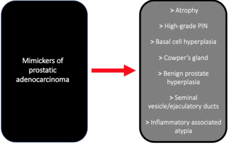
Therefore, a number of other lesions and conditions (Figure 2.3) associated to the prostate must be considered within the context of cancer diagnosis, since they are mimickers of prostate adenocarcinoma [28, 32, 33]. Of these, Benign Prostatic Hyperplasia (BPH), atrophy, and Prostatic Intraepithelial Neoplasia (PIN) must be highlighted.
Figure 2.3: Lesions and structures that can simulate prostate cancer. Some of these lesions are common differential diagnoses of prostate adenocarcinoma.
BPH (shown in Figure 2.4) is one of the most common diseases in men from 40 years onwards, probably due to the alterations in hormone balance. It produces obstruction to bladder outflow and as a result of pressure effects on the proximal conducting system of the urinary tract [11]. Microscopically, BPH is characterised by the development of a number of nodules, which can have different origins - stromal, glandular or mixtures thereof. Nodules formation is expected to be detected more often in specimens from prostate excision, instead of from biopsies. In the latter, these nodules are sometimes misdiagnosed as adenocarcinoma [33, 34].
Figure 2.4: BPH foci in (a) low magnification and in (b) in high magnification. The intraluminal infoldings within the glands is charcteristic of BPH. (c) Epithelium predominant round nodule is typical in BPH. A small sample of this nodule discovered in a biopsy could be misdiagnosed as prostate adenocarcinoma.
Atrophy - Figure 2.5 - is a common age-related benign condition, most frequently seen in peripheral zones samples. Any subtype of atrophy is expected to show basal cells, however their detection in some biopsies may be difficult [35] - Figure 2.6.
(a) (b)
Figure 2.5: Low magnification of different patterns of atrophy. (a) Acinar atrophy. (b) Cystic atrophy.
Figure 2.6: Atrophic prostate carcinoma may be occasionally cystic and resembling a focus of benign atrophy.
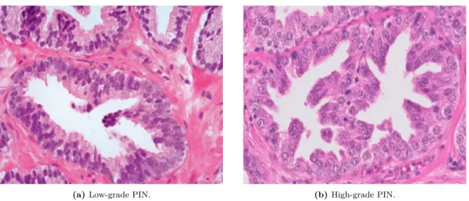
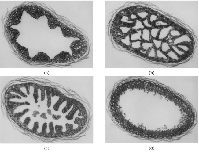
PIN refers to multiple foci of cytologically atypical luminal cells overlying diminished number of basal cells in prostatic ducts and is a forerunner of invasive prostatic carcinoma [11]. According to the cytologic characteristics of its cells, PIN may be classified into low grade PIN and high-grade PIN (Figure 2.7). The former is composed of enlarged cell nuclei, which vary in size and have a slightly increased chromatin content. The latter is characterised by cells with large nuclei of uniform size and prominent nucleoli - similar to those of carcinoma cells . The basal cell layer is intact on lower grade PIN, but may present disruption in higher grade PIN [36]. PIN can be erroneously evaluated as carcinoma or vice-versa [28], especially because there are a specific type of carcinoma which morphologically resemble PIN, the PIN-like ductal carcinoma Figure 2.8. The four different types of high-grade PIN are represent in Figure 2.9: tufting, micropapillary, cribriform and flat.
When several of the above-mentioned cancer features are detected in a specimen, the diag-nosis of prostatic adenocarcinoma can be confidently performed and a classification prognostic grade - the Gleason Score - is reported. The Gleason score system, developed in the 1960s to determine the aggressiveness of the cancer, is based on glandular architecture, which can be divided into five patterns of growth or grades. Pattern 1 lesions consist of nodules of small, well-defined glands with limited infiltration of the surrounding tissue. In contrast, pattern five
(a) Low-grade PIN. (b) High-grade PIN.
Figure 2.7: High power view of the different PIN categories: low grade and high-grade.
Figure 2.8: Example of carcinoma of the prostate, which resembles a PIN foci. It is denominated PIN-like ductal carcinoma.
lesions consist of layers of malignant cells with no discernible glandular differentiation and which are widely infiltrative. Due to the fact that most tumours are highly variable, including two or more components of these patterns, the Gleason score is, therefore, obtained by adding two sub-grades: primary and secondary grades [37]. The primary grade is assigned to the dominant pattern of the tumour, while the secondary is assigned to the subordinate pattern - for instance Gleason score 4+3.
Although changes to this grading system have been implemented to this grading system, with complementary group grades being adopted, the Gleason score system remains as one of the most significant factors in the clinical decision-making process, not only in biopsy specimens, but also mainly after a radical intervention is performed, being a predominant tool in outcome prediction [38].
2.1.2.3 Prostate Cancer Treatment
After combining the results of the PSA, DRE and histological grade of the biopsy specimen, the stage and nature of the cancer is determined. If the tumour has metastasized beyond the
(a) (b)
(c) (d)
Figure 2.9: Schematic illustration of architectural patterns of high-grade PIN. (a) The tufting pattern shows undulating mounds and heaps of cells protruding into the lumen. (b) The micropapillary pattern shows delicate finger-like projections, often with bulbous tips, with or without flbrovascular cores. (c) The cribriform pattern shows a sieve-like pattern. (d) The flat pattern shows one or two layers of cells. Adapted from [39]
prostate gland, additional tests might have to be performed, including Magnetic Resonance Imaging (MRI), bone scan, Computed Tomography (CT) and TransRectal Ultrasound (TRUS). These techniques provide relevant information, as far as accurate staging is concerned, both in local and advanced disease. If a patient is found to have advanced disease with extended involvement of surrounding structures - SVI, perineural and lymphovascular invasion - a radical treatment would be an inappropriate approach to employ, since it would unnecessarily endanger the patient while burdening healthcare resources [3]. In these cases, radiation therapy, androgen-deprivation treatments and chemotherapy are the therapies of choice. Nevertheless, advanced prostate cancer remains an incurable disease and new alternative treatments are required.
Conversely, when the diagnosis reveals localised PCa, a prostate confined tumour with no extension to the seminal vesicles, regional lymph nodes, or distant site, he is a candidate for surgical prostatectomy. This procedure is the standard first-line treatment with curative intent [27, 40]. The perceived advantage of radical prostatectomy is that, the entire prostate, where the tumour is confined, is surgically removed, aiding towards the reduction of the metastasis risk [41]. Moreover, with the recent introduction of robotics in minimally invasive surgery, enhanced treatment performance has been reported. Robotic assisted laparoscopic radical prostatectomy has gained acceptance among urologists and patients, not only because it allows the surgeon to perform complex surgical procedures with both dexterity and minimal fatigue, but mainly because it is a less invasive procedure, diminishing operative time, blood loss and hospitalisation
time. Suggestion of earlier improved erectile function and full sexual health, after robotic surgery have also been reported [42, 43].
However, despite the improved results of these robotic surgeries, cancer recurrence is a concern for men undergoing definitive treatment with curative intent for localised PCa [44]. Of all patients treated with radical prostatectomy, approximately 35% are reported to experience a re-emergence of PSA serum, after its total abrogation: a state known as BioChemical Recurrence (BCR) [45, 46]. A detectable PSA level implies residual prostate tissue and, most likely, recurrent PCa.
Considering the above, the history of BCR following surgery is highly variable, since PSA re-lapse has different meanings according to clinicopathological features - such as: Gleason Score, clinical stage and surgical margins status [47]. Therefore, it is of paramount importance to treating physicians, to assess both, 1) whether BCR is going to emerge after surgery, and 2) distinguish different biochemical recurrence based on preoperative and/or postoperative pa-rameters. The outcome prediction information will aid towards clinical decision-making, by implementing the golden complementary therapies, achieving, thus, a more personalised and cost-effective treatment regimen.
2.1.3 Prostate Cancer Biochemical Recurrence Prediction
A method capable of forecasting recurrence is highly desirable, due to the complexity of PCa disease and the associated decision-making process. Therefore, accurate estimates of the likelihood of cancer diagnosis, stage, clinical significance, treatment success, complications, and long-term morbidity are essential for patient counselling and informed decision-making. By un-derstanding the most probable endpoint of a patient’s clinical course, physicians may modify treatment and post-treatment strategies, in order to balance benefits and adverse effects of a specific therapy. Prediction also allows patients to choose responsibly among the different treat-ment strategies, proposed by the clinicians, which, ultimately, may improve their satisfaction after treatment [48].
Traditionally, physician judgement is the basis for risk estimation, patient guidance, and decision-making. However, clinicians’ estimates are often biased due to both subjective and objective confounders [49–51]. To overcome these limitations and to obtain more accurate pre-dictions, researchers have developed predictive tools – directed at predicting the probability of an outcome of interest for the individual patient, without considering the effect of time [52].
Currently, clinical prognosis of PCa relies on the evaluation of histology sections under a microscope, which allows the pathologist to determine specific tumour characteristics: Gleason score, capsule invasion, extra capsular extension, surgical margins, SVI, lymph node invasion. These features serve as variables in the widely-validated Kattan nomogram [53, 54] and CAPRA-S score [55] predictive methods, considered as the best performing tools for prostate outcome prediction after radical prostatectomy. Although these nomograms remain the most widely used tools in clinic, as far as postoperative clinical management is concerned [41], their modest overall accuracy is further devalued by the realisation that these tools largely fail in the most common cohort in the modern era (mid-grade, confined disease with moderate PSA level) [56, 57]. A tendency to overestimate the likelihood of disease recurrence for lower risk patients [55, 57] has also been reported. Hence, and in addition to these obvious generalisation and complexity limitations [58, 59], the lack of periodic updates to reflect changes in patient and
disease characteristics may compromise the applicability of some models to contemporary patient populations. To illustrate this point, the surgical procedure currently employed is Robotic-Assisted Radical Prostatectomy (RARP), as opposed to the invasive laparoscopic or open radical Prostatectomy previously adopted (until around 2010) [60, 61]. This consideration is likely to influence the outcome prediction.
While most prognostic efforts have focused on incorporating additional clinical variables, which has not significantly improved predictions [62], the potential of digital histologic images has not, yet, been fully explored. An unanswered question is whether these tools for outcome prediction could be bypassed by novel machine learning techniques, with the power to directly learn the prognostically relevant features in microscopy digital images of the tumour, without prior identification of the known tissue entities [63], e.g. Gleason score, mitoses, infiltrating immune cells, tumour budding.
Therefore, in this dissertation, and in particular in Section 2.2, emerging techniques such as digital pathology and deep learning will be exploited in order to overcome the shortcomings observed in the tools currently used to predict BCR. While digital pathology allows digitisation of the histopathology image and its consequent quantitative analysis, deep learning has the power to enhance information that cannot be perceived by the human eye. It is expected that a model resulting from the combination of these techniques has the power to predict the occurrence of relapse in patients treated with radical prostatectomy.
2.2
Anatomic Pathology
In this section the field of anatomic pathology will be detailed. In first place, the fundamen-tals of anatomic pathology will be explained. Then, the role of an emerging technique as digital pathology will be discussed and their advantages and limitations presented. Finally, approaches using deep learning applied to histopatholgy in precision medicine will be presented and some image classification examples for prostate cancer will be detailed.
2.2.1 Fundamentals of Anatomic Pathology
Interpreting images of tissues and cells at a resolution higher than the naked human eye is the core of pathology (also referred to as histopathology or anatomical pathology). This medical specialty is fundamental to studying, understanding and diagnosing disease, while providing further insight into what is required for a successful treatment.
As disease processes occur at the molecular/cellular levels, its manifestations and mechanisms can be observed at the tissue level using a microscope. In order to do so, several steps from the acquisition of the sample to the final diagnosis, must be completed (Figure 2.10).
The clinical histology process begins when the portion of tissue to be studied is extracted from the patient. Several possible approaches to collect tissue are possible, including fine-needle aspiration, fine-needle biopsy, excisional biopsy or excision of the entirety of the lesion. The sensitivity (i.e. the likelihood of getting the correct diagnosis) and specificity (i.e. the likelihood of not getting the incorrect diagnosis) increase from fine-needle aspiration to excision of the entire lesion, since the larger the biopsies, the more cellular content is preserved. Hence, the pathologist is able to examine multiple slides from different regions of the sample. In order to stop tissue degradation and prevent microorganisms growth, fixation of the sample, usually accomplished with formalin, must be performed [64].
Afterwards, the tissue is physically and chemically stabilized, during the processing phase, where water intrinsically contained within the tissue is removed, and a hardening agent (paraffin) is infiltrated within the tissue, allowing the sample to become firm. During the embedding phase, the sample is inserted into a block of support rigid mould. The result is a tissue block which can now be sliced into thin sections (3-10 µm thickness). At this point, the tissue slices are nearly invisible under a light microscope and must be stained to create contrast. The most widely used staining method, both for diagnostic and research purposes, is Hematoxylin and Eosin (H&E). H&E histological staining protocol differentiates structures according to their pH. Specifically, hematoxylin, of a basic nature has affinity for acid/basophilic substances, such as nucleic acids (DNA, RNA). In contrast, eosin has affinity for basic/acidophilic structures, of which cytoplasm is an example. Hence, when a biological sample stained with H&E is observed under a microscope, the cell nuclei have a blue-purple hue, whereas cytoplasms have shades in a range from pink to red. The final result, following all of these processes, is a slide or set of slides prepared to be visualised and analysed under a microscope by a pathologist [64–66].
2.2.2 Digital Pathology
Since the 19th century, pathologists have been using the microscope as the primary tool to observe stained specimen on the slide glasses. They rely on the microscope, since it has the power to provide live images at increased resolution [67]. However, after the development of the first automated, high resolution Whole-Slide Imaging (WSI) system by Wetzel and Gilbertson in 1999, interest in using WSI for different applications in pathology practice has steadily grown [68, 69]. This process was catalysed by changes in imaging hardware, as well as, growth in com-putational power accompanied by faster and increased data storage and declining comcom-putational costs [70].
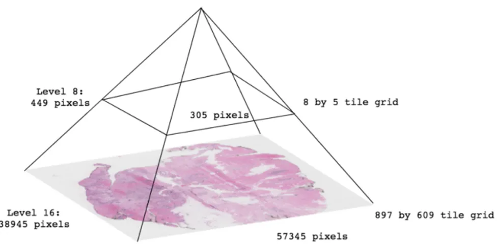
The integration of digital technologies systems in anatomic pathology departments offers benefits, not only in terms of quality, but also efficiency [71]. WSI – the digitisation of glass slides – produces high resolution digital images, involving relatively high speed digitisation of glass slides of different samples (e.g. tissue sections, smears), scanning them at multiple magnifications and focal planes (x, y and z axes) [72]. Essentially, a whole slide image consists of a pyramid of tiled images, with various levels corresponding to a specific magnification of the image - Figure 2.11.
Figure 2.11: Pyramid structure representing the various resolutions that compose a whole slide image. Adapted from [73].
Interactive software for visualisation enables the slides to be examined on a computer screen, allowing the pathologist to freely navigate the image over a complete range of standard and in-between magnifications and perform, therefore, tasks that have historically been carried out with a light microscope. Digital platforms are very useful for sharing cases both locally and internationally and to provide expertise to remote locations. Consultation for difficult cases is, also, possible within hours instead of days to weeks for cases sent through regular mail. In addition to this, providing a digital record of the exam to the patient, while maintaining the original physical glass slides in archive is a tremendous advantage, as far as clinical management is concerned. A typical digital pathology set-up is shown in Figure 2.12.
Digital slides, in contrast to glass slides, can be easily annotated and regions of interest identified and associated to the written report. Instead of just replacing the microscope for diagnostic purposes, digital pathology provides improved quantification analysis of histopatho-logical images, which are tasks highly affected by subjectivity. These image analysis techniques are more reproducible than traditional microscopy for quantitative measurements [74].
Recently, the US Food and Drug Administration (FDA) cleared the marketing of the first WSI system for digital pathology [75]. This opens a new era for the introduction of compu-tation components into each diagnosis process. Moreover, the digitization of high-resolution whole slide images makes it possible to implement Computer Aided Diagnosis (CAD) system to analyze large-scale image data, thus alleviating intra- and inter-observation variations among pathological experts and achieving statistical conclusions across hundreds of slides [76]. Digital pathology is regarded as the required “bridge” to apply artificial intelligence algorithms to whole slide images which has the potential to greatly improve clinical practice.
2.2.2.1 Intel ligent Digital Pathology
The promise of digital pathology is not, however, the simple transfer of an image from a glass slide to a monitor, not even the flexibility of distribution and modification of the image, but instead the potential to enhance the pathologist’s assessment with information and intelligence that cannot be perceived by human examination. Moreover since most pathology diagnosis are, currently, based on the subjective (but educated) opinion of pathologists, there is, clearly, a necessity for quantitative image-based assessment of digital pathology slides.
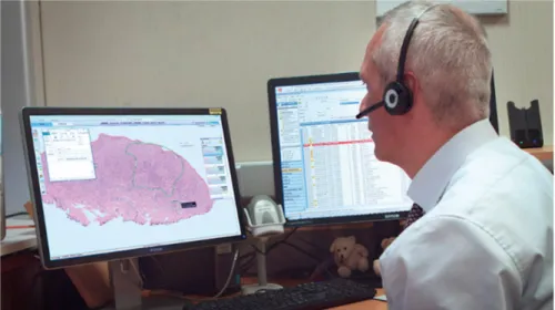
Figure 2.12: Digital pathology workstation. The microscope has been replaced by a high resolution computer screen where the pathologist is able to view digitally scanned slides. Adapted from [74].
since the preparation process preserves the underlying tissue architecture [77]. As a result, a detailed spatial interrogation (e.g. capturing nuclear orientation, texture, shape, architecture) of the entire tumour morphological landscape and its most invasive elements can be deduced only from a histopathology image. The additional complexity and density in these images, while providing a wealth of information, is ideally suited to power automated computed algorithms. The application of these algorithms is essential, not only from a diagnostic perspective, in order to understand the underlying reasons for the rendering of a specific diagnosis (e.g. specific chromatin texture in the cancerous nuclei which may indicate certain genetic abnormalities), but also for research applications (e.g. to understand the biological mechanisms of the disease process and ultimately to improve diagnosis and treatment procedures). Consequently there has been substantial interest in the digital pathology image analysis community to develop algorithms and feature identification approaches for automated tissue classification, disease grading and also developing histologic image-based companion diagnostic tests for predicting disease outcome and precision medicine [78].
Recently, a breast cancer multi-classification method using a newly proposed deep learning model was reported [79]. Instead of just focusing on the binary classification (positive or negative for malignancy), these authors further explore quantification to obtain different tumour sub-classes within benign and malignant conditions (e.g. ductal carcinoma, lobular carcinoma, adenosis, fibroadenoma,. . . ). The model used data from a large-scale dataset – BreaKHis [80] – achieving a remarkable performance (average 93.2% accuracy), when compared to previous reported techniques.
Coudray et al trained a deep convolutional neural network (Inception v3) to automatically analyse lung tumour digital slides, and distinguish between lung adenocarcinoma, squamous cell carcinoma or normal lung tissue. The deep learning model was developed using 1634 whole-slide images available in The Cancer Genome Atlas (TCGA) [81] and tested on independent cohorts in-house collected. Performance of the reported method was comparable to that of pathologists, with an average Area Under the Curve (AUC) of 0.97 [82].
Moreover, a predictive tool resulting from the combination of convolutional and recurrent architectures was recently developed to predict colorectal cancer outcome. This approach was
based on digitised tumour tissue samples from 420 patients, without any intermediate tissue classification. The results show that deep learning-based outcome prediction outperforms visual histological assessment performed by human experts in the stratification into low- and high-risk patients [83].
For automated Gleason PCa grading, Arvanati et al has recently reported a deep learning approach to analyse prostate digital samples. A convolutional neural network was trained us-ing detailed Gleason annotations on a cohort of 641 patients and was then evaluated on an independent test cohort of 245 patients annotated by two pathologists. The model’s Glea-son score achieved pathology expert-level stratification of patients into prognostically distinct groups. Overall, this shows promising results regarding the applicability of deep learning-based solutions towards more objective and reproducible PCa grading, in contrast with a human sub-jective evaluation, especially for cases with heterogeneous Gleason patterns [84].
These and other recent studies [78, 85–89] suggest that state of the art deep learning tech-niques applied to digital slide images can improve diagnostic accuracy and efficiency. It can also provide features correlated with prognosis that a human observer cannot perceive. As these and more studies unfold, digital pathology will undoubtedly open up new avenues for computational exploration of individual disease tissues. With the emerging of deep learning tools, and many available pre-trained networks, the accurate prediction of a disease outcome – which is one of the most interesting and challenging tasks for physicians in the cancer medical field – will start to be accomplished. Ultimately, better disease surveillance, earlier detection, more accurate and consistent diagnosis and prognosis will create an era of truly personalised medicine.
2.3
Deep Learning
The present section is dedicated to providing insights about deep learning. Firstly the ba-sic concepts of neural networks, the basis of deep learning, will be presented and the rest of the chapter is dedicated to CNN, a special type of neural networks, which has been success-fully employed in different tasks, involving processing data with grid-bases structure, especially images.
2.3.1 Basic Concepts of Neural Networks
Deep learning offers a different perspective on feature learning and representations, where robust, abstract and invariant features are learnt end-to-end, hierarchically, from raw data [90]. Despite being a subfield of machine learning, the key difference is on how features are extracted. While traditional machine learning approaches depend on handcrafted engineering features, deep learning algorithms have the power to learn a set of optimal features automatically/user-independently. This means that these algorithms automatically perceive the relevant features required for the solution of the problem. Deep learning is inspired by artificial neural networks (ANN), - or simply neural networks - which in turn are biologically inspired algorithms. The term network is named after the topology, since neural networks are represented by composing many different layers together. A network composed of three layers connected together in a chain structure is represented in the following figure - Figure 2.13.
Figure 2.13: Architecture of simple neural network. It is composed of 3 layers: input layer, hidden layer and output layer. The input layer receives the input data, a vector of N elements, in this case N = 3. The hidden layer is composed of four units, thus the width of the model is four. The output layer computes the answer of the network from the hidden representation.
The first layer of a neural network is called the input layer, while the last layer is called the output layer. The former holds values of the input vector and the latter holds the final results provided by the model. The layers between the input and output are named hidden layers. The behavior of these layers is not directly specified by the training data i.e. the learning algorithm must decide how to use these layers to best implement an approximation to the desired output. The overall number of hidden layers indicates the depth of the model - thus the term deep -, while their dimensionality (i.e. number of neurons) determines the width of the model.
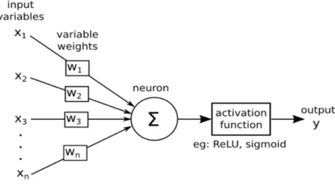
The fundamental component of neural networks is the artificial neuron, named node or unit. Just as in biological neurons, an artificial neuron takes in a vector of inputs x = [x1x2x3... xn]
each of which is multiplied by a specific weight w = [w1w2w3... wn] and an activation function φ is applied. The output of the neuron is expressed as:
y = f (x) = φ(x · w + b) (2.1) where b is the bias term. Weights and biases are the neuron’s parameters, and their values are determined in the process of learning. A schematic representation of an artificial neuron is shown in Figure 2.14. The activation function decides whether a neuron should be activated or not, i.e. whether the information that the neuron is receiving is relevant or whether it should be ignored. The purpose of the activation function is to introduce nonlinear properties, allowing the network to learn from highly complex functions, instead of just computing linear functions (e.g. the linear transformation of the input by the weights and biases).
As far as activation functions are concerned, the most commonly used types are Sigmoid, Tanh, Rectified Linear Unit (ReLU) and Leaky ReLU. However, ReLU is the function adopted in the majority of the deep learning models, since it is computationally economical compared to the remaining alternatives and has proven to successfully work in a wide range of different cases.
Figure 2.14: Schematic representation of an artificial neuron, whereP
= x · w + b.
As far as the information flow is concerned, different models are distinguished in neural networks: feedforward and recurrent neural networks. In feedforward networks, information flows from the input to the output through the different network layers and without feedback connections. If those connections are present and intermediate outputs are redirected back to previous layers or stored for later use, the network is called recurrent. Since only feedforward networks are used in this study, the following sections concern only this type of networks.
2.3.2 Training a Neural Network
Training a neural network, i.e. learning the values of the parameters (weights and biases) is the essential part of deep learning and is accomplished by solving an optimisation problem. In order to solve this optimisation problem, gradient-based algorithms are used and the weights of the model are updated using the backpropagation algorithm [91].
The first phase is the forward-propagation, which occurs when the network is exposed to the training data and these cross the entire neural network in order to calculate the predictions (labels). In detail, the input data is passed through the network in such a way that all the neurons apply their transformation to the information they receive from the neurons of the previous layer and send it to the neurons of the next layer. When the data has crossed all the layers, and all its neurons have made their calculations, the final layer will be calculated with a result of label prediction for the original input samples.
Afterwards, a loss function - often called the objective function, cost function, or simply error - must be chosen. This function is used to evaluate to what extent the output is correctly predicted, i.e. it quantifies how good or bad the prediction result is, when compared to its known label. Ideally, the cost function would be zero, meaning that there is no divergence between the estimated value and the expected value. Typically, for classification problems the cross-entropy loss is the most commonly used loss function. Once the loss has been computed, this infor-mation is propagated backwards in order to improve the model predictions. Hence, the name of the algorithm: backpropagation. Starting from the output layer, that loss is propagated to calculate the gradient of the loss function with respect to each neuron of weights or parameters. Thereafter, these parameters - weights - are updated in the opposite direction of the gradient of the loss function. Different variants of gradient descent algorithm have been proposed,
includ-ing Stochastic Gradient Descent (SGD), Adaptive gradient (Adamgra) and Adaptive moment estimation (Adam). The Adam optimiser - derived from the Adamgrad - is very similar to the SGD, however, instead of maintaining a single learning rate for all weight updates it computes and uses individual adaptive learning rates for different parameters from estimates of first and second moments of the gradients.
This process is then repeated for each example of the dataset and the weights of the inter-connections of the neurons will be gradually adjusted until good predictions are obtained, i.e. until a minimal loss error is reached.
2.3.2.1 Hyperparameters Tuning
In addition to the weight parameters defined within the network, deep learning algorithms also require additional parameters to carry out the learning process. These hyperparameters highly influence the algorithm performance and must, therefore, be wisely selected.
In order to update the weights of the model, a number of samples from the training dataset must be used to calculate the error: this hyperparameter is denominated batch size. The batch size is a hyperparameter that defines the number of samples to go through before updating the internal model parameters. The batch size has an effect on the resource requirements of the learning process. A large batch size (sometimes equal to the entire dataset) allows computational boosts, but at the expense of more memory for the training process. A small batch size is advantageous since it prevents the training process from stopping at local minima, but it is also considerably more prone to noise during the error calculations. The optimal size will depend on many factors, including the available memory capacity, as well as the size of training dataset.
Once the loss gradient has been estimated, the derivative of the error can be calculated and used to update the weights of the network through:
wnewi = woldi − γ ∗ ∂L ∂wi
(2.2) where winew and wiold are the current and previous weights respectively, ∂w∂L
i is the gradient
of the loss function (in this one-dimension case, it will be the first derivate of loss function with respect to only one weight) and γ is the learning rate. The learning rate controls at which pace the weights are updated. The optimal value for the learning rate depends on the problem under study. In general, if it is too large, the learning process is fast - since big steps are being made at each iteration, however, in this case, the minimum value is likely to be missed, making it almost impossible for the algorithm to converge. Conversely, if the learning rate is small, small advances will be made at each iteration, improving the likelihood of smoothly reaching a local minimum. Nevertheless, this can cause the learning process to be too slow.
Finally, the training process must be repeated several times until a good or good enough set of model parameters is discovered. The total number of iterations of the process is bounded by the number of complete passes through the data after which the training process is complete. This is referred to as the number of epochs. The optimal number of epochs can be reached using, for instance, a strategy of imposing a condition, e.g. epochs stop when the error is close to zero.
![Figure 2.2: Zonal anatomy of the normal prostate as described by McNeal [7–9]. The transition zone comprises only 5%–10% of the glandular tissue in the young male](https://thumb-eu.123doks.com/thumbv2/123dok_br/15463954.1031882/22.892.245.652.460.697/figure-anatomy-prostate-described-mcneal-transition-comprises-glandular.webp)