Quantitative analysis of contamination of biological origin in direct detection in-situ

Maria Carolina Trindade Gonçalves

[Nome completo do autor]

[Nome completo do autor]

[Nome completo do autor]

[Nome completo do autor]

[Nome completo do autor]

[Nome completo do autor]

[Nome completo do autor]

Bachelor of Science in Biomedical Engineering

[Habilitações Académicas]

[Habilitações Académicas]

[Habilitações Académicas]

[Habilitações Académicas]

[Habilitações Académicas]

[Habilitações Académicas]

[Habilitações Académicas]

Quantitative analysis of contamination of biological

origin in direct detection in-situ

[Título da Tese]

Advisor: Valentina Vassilenko, Assistant Professor, FCT/UNL

Advisor: Mário Diniz, Assistant Professor, FCT/UNL

Dissertation to obtain the Master Degree in

Biomedical Engineering

Júri:

Presidente: Doutora Carla Maria Quintão Pereira, Profes-sora Auxiliar da Universidade NOVA de Lis-boa - Faculdade de Ciências e Tecnologia Arguente: Doutora Susana Maria Pereira Gaudêncio de

Matos, Investigador Auxiliar da Universidade NOVA de Lisboa - Faculdade de Ciências e Tecnologia

Vogal: Doutora Valentina Borissovna Vassilenko, Professora Auxiliar da Universidade NOVA de Lisboa - Faculdade de Ciências e Tecnologia,

Quantitative analysis of contamination of biological origin in direct detection

in-situ

Copyright © Maria Carolina Trindade Gonçalves, Faculdade de Ciências e

Tec-nologia, Universidade Nova de Lisboa.

A Faculdade de Ciências e Tecnologia e a Universidade Nova de Lisboa têm o

direito, perpétuo e sem limites geográficos, de arquivar e publicar esta

disserta-ção através de exemplares impressos reproduzidos em papel ou de forma digital,

ou por qualquer outro meio conhecido ou que venha a ser inventado, e de a

di-vulgar através de repositórios científicos e de admitir a sua cópia e distribuição

com objetivos educacionais ou de investigação, não comerciais, desde que seja

dado crédito ao autor e editor

Acknowledgements

First of all I would like to thank my advisors, Professor Valentina Vassilenko, for the opportunity to work in such an interesting project and for her enthusiasm, and Pro-fessor Mário Diniz, for the constant availability, help and dedication and for all the trans-mitted knowledge in a fascinating area such as Microbiology.

I would like to thank my lab partners for making the lab a livelier place, especially to Paulo Santos for all the help and humour and Jorge Fernandes for revising my work and for all the helpful insight.

To all my friends and particularly to Cláudia for the company throughout the long days and even longer nights working on this thesis and for the great sense of humour that always brightened the darkest hours. Thank you for always being there.

To João for all the support (I always remember the times you brought me choco-late) and for never letting me give up. Thank you for all your patience throughout these last months, I know it was not easy.

Last but not least, to my parents and my brother, who have always been there for me, for their endless support, encouragement and love. This thesis would not have been possible without them.

Abstract

Fast detection of biological contaminations is of great importance in numerous ar-eas of human health, such as, toxicology, environmental health and medicine. Currently, this is one of the top concerns of space agencies, since the duration of manned missions is becoming increasingly longer and the conventional methods for biological contami-nations and treatment are unavailable while in space.

Microorganisms have been shown to proliferate under punishing environments as the ones suffered in space. This, associated with the astronauts’ weakened immune sys-tem, may originate serious health problems.

The need for finding sample retrieving methods in situ and techniques for fast and online detection of biological contamination is very important, not only for preventing infections but also for pursuing the indicated treatment. The technique used in this work was the Ion Mobility Spectrometry coupled with Gas Chromatography (GC-IMS). This is an analytical technique that identifies organic compounds in the gaseous phase.

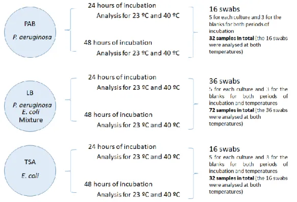
In order to check if it is possible to identify bacteria based on the volatile organic compounds (VOCs) released by them, two bacteria were studied: Escherichia coli (ATCC 25922 pCU18) and Pseudomonas aeruginosa (ATCC 27853). Cultures of each bacteria indi-vidually and in a mixture were made and a bacterial sample was retrieved by swabbing. The cotton swab was then sealed in a vial. The vial’s headspace was analysed with the IMS equipment.

The objective of this thesis was to find a pattern of released bacterial VOCs that allowed their identification. This work indicates that it is possible to identify these bac-teria based of their released VOCs profile, even when they are in a mixture.

This findings pave the way for a faster detection and identification method for biological contaminations. In the future, this technique may also be applied in other con-texts, such as, in a hospital, and with other microorganisms.

Resumo

A deteção rápida de contaminações biológicas é de grande importância em várias áreas da saúde humana como sejam, toxicologia, saúde ambiental e medicina. Atual-mente, esta é uma das principais preocupações das agências espaciais, pois a duração das missões tripuladas está a aumentar e não é possível recorrer aos métodos convenci-onais de deteção de contaminações e do tratamento.

Há microrganismos que conseguem prosperar em condições hostis como as que se fazem sentir no espaço. Isto, associado ao sistema imunitário debilitado dos astronautas, pode causar graves problemas de saúde.

Encontrar métodos de recolha de amostras biológicas in-situ e técnicas para a sua rápida análise é muito importante, não só para prevenir infeções como para seguir o tratamento adequado. A técnica usada neste trabalho foi a Espectrometria de Mobili-dade Iónica associada a Cromatografia Gasosa (GC-IMS). Esta é uma técnica analítica utilizada para identificar compostos no estado gasoso.

De modo a verificar a possibilidade de identificação de bactérias com base nos compostos orgânicos voláteis (VOCs) que libertam, duas bactérias foram estudadas: Escherichia coli (ATCC 25922 pCU18) e Pseudomonas aeruginosa (ATCC 27853). Foram fei-tas culturas de ambas as bactérias e da mistura das duas. A amostra foi retirada das culturas com uma cotonete que foi posteriormente colocada num frasco. O ar do frasco foi retirado para análise pelo equipamento de GC-IMS.

O objetivo desta tese era encontrar um padrão composto por VOCs libertados pe-las bactérias que permitisse a sua identificação. Foi possível encontrar um padrão para as bactérias que permitiu ainda identificá-las separadamente na mistura das duas.

Estes resultados indicam que com este método é possível identificar contamina-ções biológicas mais rapidamente. No futuro, pode ser aplicado em outros contextos, como hospitais, e para outros microrganismos.

Contents

1 INTRODUCTION ... 1

OBJECTIVES ... 2

2 MICROBIOLOGY ... 3

VOCS EMITTED BY BACTERIA ... 7

SAFETY MEASURES ... 10

3 STATE OF THE ART ... 13

4 ION MOBILITY SPECTROMETRY ... 19

PRODUCTION OF REACTANT IONS ... 21

PRODUCTION OF PRODUCT IONS ... 22

GAS CHROMATOGRAPHY... 24

5 DEVELOPMENT AND APPLICATION OF A METHOD FOR DETECTION AND IDENTIFICATION OF BACTERIAL VOCS ... 27

EXPERIMENTAL SETUP ... 27

GC-IMS device...28

Spectra ...29

LAV software ...30

Preparation of the sample ...32

PREVIOUS PROTOCOL USING MCC-IMS ... 32

OPTIMIZATION OF THE PARAMETERS ... 33

EXPERIMENTAL PROCEDURE ... 35

BACTERIA AND CULTURES MEASURED ... 36

6 RESULTS AND DISCUSSION ... 39

xii

RELEVANT VOC CHARACTERIZATION ... 68

7 CONCLUSIONS AND FUTURE WORK ... 71

FUTURE WORK ... 72

8 BIBLIOGRAPHY ... 73

1 APPENDIX A – CULTURE MEDIUM PREPARATION ... 79

2 APPENDIX B – BACTERIAL SAMPLE PREPARATION... 81

List of Figures

FIGURE 2.1 – MOST COMMON MORPHOLOGICAL SHAPES OF BACTERIAL CELLS ... 4

FIGURE 2.2 – SCANNING ELECTRON MICROGRAPH OF PSEUDOMONAS AERUGINOSA. ... 5

FIGURE 2.3–COLORIZED SCANNING ELECTRON MICROGRAPH OF ESCHERICHIA COLI ... 6

FIGURE 4.1–SCHEMATIC DESIGN OF THE IMS PART OF THE DEVICE... 20

FIGURE 4.2 - CROSS SECTION OF A MULTI-CAPILLARY COLUMN... 24

FIGURE 4.3 – SCHEMATIC VIEW OF SAMPLE SEPARATION PERFORMED BY A MULTI-CAPILLARY COLUMN ... 25

FIGURE 4.4 - SCHEMATIC DIAGRAM OF AN IMS EQUIPMENT ASSOCIATED WITH A PRE-SEPARATION TECHNIQUE. ... 25

FIGURE 4.5 – SPECTRA OF A ROOM AIR SAMPLE OBTAINED USING THE LAV SOFTWARE. ... 26

FIGURE 5.1 –EXPERIMENTAL SET-UP ... 27

FIGURE 5.2-SCHEMATIC OF THE INTERNAL GASFLOW AND THE COMPOSING ELEMENTS OF THE GC-IMS DEVICE. ... 28

FIGURE 5.3–TYPICAL VIEW OF THE LAV SOFTWARE. ... 30

FIGURE 5.4 – SPECTRA WITH THE COMPARISON GREEN/RED/BLUE VIEW. ... 31

FIGURE 5.5 – PART OF THE WINDOW FROM THE GALLERY PLUGIN. ... 31

FIGURE 5.6 – WINDOW FOR THE REPORTER PLUGIN. ... 32

FIGURE 5.7 – COMPARISON BETWEEN THE SPECTRA OBTAINED IN THE GC-IMS EQUIPMENT WITH DIFFERENT CARRIER GAS FLOWS AND VALVE OPENING TIME. ... 34

FIGURE 5.8–PROGRAM USED IN THE GC-IMS TO PERFORM THE MEASUREMENTS. ... 35

FIGURE 5.9-EXPERIMENTAL PROCEDURE OF THE USED METHOD TO OBTAIN VOCS PROFILE OF BACTERIA. ... 36

FIGURE 5.10 – SCHEMATIC OF THE CULTURES MADE IN EACH MEDIA AND THEIR INCUBATION PERIODS. ... 37

FIGURE 6.1 – RELEVANT PEAKS FOUND AFTER 24 HOURS OF INCUBATION FOR P. AERUGINOSA AT 23 ºC (LEFT) AND 40 ºC (RIGHT) IN THE NUTRIENT MEDIUM LB.. ... 40

FIGURE 6.2 - DESIGN CREATED BY THE COMMON PEAKS FOR P. AERUGINOSA AFTER 24 HOURS OF INCUBATION IN LB GROWTH MEDIUM AT BOTH TEMPERATURES.. ... 41

FIGURE 6.3 – CHARACTERISTIC SPECTRA OF THE BLANK AND THE CULTURE OF P. AERUGINOSA AT 23 ºC AND 40 ºC AFTER 24 HOURS OF INCUBATION. ... 43

FIGURE 6.4-RELEVANT PEAKS FOUND AFTER 48 HOURS OF INCUBATION AT 23 º C(LEFT) AND AT 40 ºC(RIGHT) FOR P. AERUGINOSA IN THE NUTRIENT MEDIUM LB. ... 43

xiv

FIGURE 6.6 - CHARACTERISTIC SPECTRA OF THE BLANK AND THE CULTURE OF P. AERUGINOSA AT 23 ºC AND 40 ºC

AFTER 48 HOURS OF INCUBATION. ... 46

FIGURE 6.7-RESULTS OF THE ANALYSIS FOR E. COLI IN THE LB GROWTH MEDIUM, AFTER 24 HOURS OF INCUBATION.. ... 48

FIGURE 6.8 - DESIGN CREATED BY THE COMMON PEAKS FOR E. COLI AFTER 24 HOURS OF INCUBATION IN LB GROWTH MEDIUM. ... 49

FIGURE 6.9 - CHARACTERISTIC SPECTRA OF THE BLANK AND THE CULTURE OF E. COLI AT 23 ºC AND 40 ºC AFTER 24 HOURS OF INCUBATION. ... 50

FIGURE 6.10–RESULTS OF THE ANALYSIS FOR E. COLI IN THE LB GROWTH MEDIUM, AFTER 48 HOURS OF INCUBATION. ... 51

FIGURE 6.11 – DESIGN CREATED BY THE COMMON PEAKS FOR E. COLI AFTER 48 HOURS OF INCUBATION IN LB GROWTH MEDIUM. ... 52

FIGURE 6.12 - CHARACTERISTIC SPECTRA OF THE BLANK AND THE CULTURE OF E. COLI AT 23 ºC AND 40 ºC AFTER 48 HOURS OF INCUBATION. ... 53

FIGURE 6.13 – RELEVANT PEAKS FOR THE BACTERIAL MIXTURE IN THE LB GROWTH MEDIUM AFTER 24 HOURS OF INCUBATION AND AT 23 ºC.. ... 55

FIGURE 6.14-CHARACTERISTIC SPECTRA OF THE BLANK,E. COLI,P. AERUGINOSA AND THE MIXTURE OF BOTH AT ROOM TEMPERATURE AFTER 24 HOURS OF INCUBATION. ... 57

FIGURE 6.15 – RELEVANT PEAKS FOUND AFTER 48 HOURS OF INCUBATION OF THE BACTERIAL MIXTURE IN LB GROWTH MEDIUM, AT ROOM TEMPERATURE.. ... 57

FIGURE 6.16 - CHARACTERISTIC SPECTRA OF THE BLANK, E. COLI, P. AERUGINOSA AND THE MIXTURE OF BOTH AT ROOM TEMPERATURE AFTER 48 HOURS OF INCUBATION. ... 59

FIGURE 6.17 – RELEVANT PEAKS FOUND FOR P. AERUGINOSA IN THE PAB GROWTH MEDIUMAFTER 24 HOURS OF INCUBATION AND FOR SAMPLE TEMPERATURE OF 23 ºC. ... 60

FIGURE 6.18–RELEVANT PEAKS FOUND FOR P. AERUGINOSA AFTER 48 HOURS OF INCUBATION. ... 62

FIGURE 6.19 - EXAMPLE OF SPECTRA OF P. AERUGINOSA. ... 63

FIGURE 6.20 - RELEVANT PEAKS FOUND AFTER 24 HOURS OF INCUBATION FOR E. COLI IN THE NUTRIENT MEDIUM TSA.. ... 64

FIGURE 6.21 – RELEVANT PEAKS FOUND AFTER 48 HOURS OF INCUBATION FOR E. COLI IN THE NUTRIENT MEDIUM TSA. ... 65

FIGURE 6.22–EXAMPLE OF SPECTRA OF E. COLI.. ... 67

FIGURE 1–GROWTH MEDIA USED DURING THE COURSE OF THIS WORK. ... 80

FIGURE 2 – SCHEMATIC OF THE STEPS TAKEN TO OBTAIN THE BACTERIAL CULTURES. ... 81

List of Tables

TABLE 2.1 – CHEMICAL STRUCTURE AND MOLECULAR FORMULA OF SOME COMPOUNDS KNOWN TO BE RELEASED BY E.

COLI AND P. AERUGINOSA. ... 8

TABLE 5.1-LIST OF THE MATERIALS USED DURING THE COURSE OF THIS WORK, AS WELL AS THEIR DIMENSION AND THEIR MANUFACTURER ... 29 TABLE 5.2 – PREVIOUSLY DEVELOPED PROGRAM USED TO PERFORM THE MEASUREMENTS. ... 33 TABLE 6.1 - RELATIVE INTENSITIES OF THE MUTUAL PEAKS FOUND FOR P. AERUGINOSA AFTER 24 HOURS OF

INCUBATION IN THE LB GROWTH MEDIA AT 23 ºC AND AT 40 ºC. ... 41 TABLE 6.2 - RETENTION TIME, IN SECONDS, AND DRIFT POSITION RELATIVE TO THE RIP OF THE PEAKS ONLY PRESENT IN THE CULTURE FOR P. AERUGINOSA IN LB GROWTH MEDIUM AFTER 24 HOURS OF INCUBATION. ... 42

TABLE 6.3- RELATIVE INTENSITIES OF THE MUTUAL PEAKS FOUND FOR P. AERUGINOSA AFTER 48 HOURS OF INCUBATION IN THE LB GROWTH MEDIA AT 23 ºC AND AT 40 ºC ... 45 TABLE 6.4 - RETENTION TIME, IN SECONDS, AND DRIFT POSITION RELATIVE TO THE RIP OF THE PEAKS ONLY PRESENT IN THE CULTURE FOR P. AERUGINOSA IN LB GROWTH MEDIUM AFTER 48 HOURS OF INCUBATION. ... 45

TABLE 6.5 - RETENTION TIME, IN SECONDS, AND DRIFT POSITION (RIP RELATIVE) OF THE PEAKS FOUND FOR THE POSSIBLE PATTERNS FOR P. AERUGINOSA GROWN IN LB GROWTH MEDIUM.. ... 47

TABLE 6.6 - RELATIVE INTENSITIES OF THE MUTUAL PEAKS FOUND FOR E. COLI AFTER 24 HOURS OF INCUBATION IN

THE LB GROWTH MEDIA AT 23 ºC AND AT 40 ºC ... 49 TABLE 6.7-RETENTION TIME, IN SECONDS, AND DRIFT POSITION RELATIVE TO THE RIP OF THE PEAKS ONLY PRESENT IN THE CULTURE FOR E. COLI IN LB GROWTH MEDIUM AFTER 24 HOURS OF INCUBATION. ... 50

TABLE 6.8 – RELATIVE INTENSITIES OF THE MUTUAL PEAKS FOUND FOR E. COLI AFTER 48 HOURS OF INCUBATION IN

THE LB GROWTH MEDIA AT 23 ºC AND AT 40 ºC. ... 52 TABLE 6.9 – RETENTION TIME, IN SECONDS, AND DRIFT POSITION RELATIVE TO THE RIP OF THE PEAKS ONLY PRESENT IN THE CULTURE FOR E. COLI IN LB GROWTH MEDIUM AFTER 48 HOURS OF INCUBATION. ... 53

TABLE 6.10 – RETENTION TIME, IN SECONDS, AND DRIFT POSITION (RIP RELATIVE) OF THE PEAKS FOUND FOR THE POSSIBLE PATTERNS FOR E. COLI GROWN IN LB GROWTH MEDIUM. ... 54

xvi

TABLE 6.12 – RETENTION TIME AND DRIFT POSITION [RIP RELATIVE] OF THE RELEVANT PEAKS FOUND FOR THE BACTERIAL MIXTURE AFTER 48 HOURS OF INCUBATION. ... 58 TABLE 6.13–RETENTION TIME, IN SECONDS, AND RIP RELATIVE DRIFT POSITION OF THE PEAKS ONLY FOUND IN THE SPECTRA FROM THE P. AERUGINOSA IN PAB GROWTH MEDIUM AFTER 24 HOURS OF INCUBATION. ... 61

TABLE 6.14 – RETENTION TIME, IN SECONDS, AND DRIFT POSITION RELATIVE TO THE RIP OF THE MUTUAL PEAKS FOUND FOR 24 HOURS OF INCUBATION AND FOR BOTH GROWTH MEDIA, LB AND PAB. ... 61 TABLE 6.15 – RETENTION TIME AND DRIFT POSITION OF THE SHARED PEAKS OF THE TWO GROWTH MEDIA (LB AND PAB) AFTER 24 HOURS OF INCUBATION. ... 61 TABLE 6.16-RETENTION TIME, IN SECONDS, AND DRIFT POSITION (RELATIVE TO THE RIP) OF THE PEAKS FOUND TO BE PRESENT IN THE CULTURE OF P. AERUGINOSA AFTER 48 HOURS OF INCUBATION AND FOR BOTH GROWTH MEDIA (LB AND PAB). ... 62 TABLE 6.17 – RETENTION TIME, IN SECONDS, AND DRIFT POSITION (RELATIVE TO THE RIP) OF THE PEAKS FOUND TO BE PRESENT IN THE CULTURE OF P. AERUGINOSA FOR BOTH PERIODS OF INCUBATION AND FOR BOTH GROWTH

MEDIA (LB AND PAB). ... 63 TABLE 6.18 - MUTUAL PEAKS AFTER A 24 HOUR PERIOD INCUBATION OF E. COLI FOR BOTH GROWTH MEDIA: LB AND

TSA. ... 65 TABLE 6.19-MUTUAL PEAKS AFTER A 48 HOUR PERIOD INCUBATION FOR E. COLI IN BOTH GROWTH MEDIA:LB AND TSA. ... 66 TABLE 6.20 – MUTUAL PEAKS TO BOTH PERIODS OF INCUBATION (24 HOURS AND 48 HOURS) AND TO BOTH GROWTH MEDIA: LB AND TSA FOR E. COLI.. ... 66

TABLE 6.21 – CALCULATED VALUES OF ION MOBILITY K (CM2_V-1_S-1_{) AND REDUCED ION MOBILITY K0 (CM}-2_V-1_S-1_{) FOR} EACH OF THE PEAKS IN THE PATTERN FOR P. AERUGINOSA... 68

TABLE 6.22 - CALCULATED VALUES OF ION MOBILITY K (CM2 _V-1 _S-1_{) AND REDUCED ION MOBILITY K0 (CM}-2 _V-1 _S-1₎ FOR EACH OF THE PEAKS IN THE PATTERN FOR E. COLI ... 69 TABLE 1–RELEVANT PEAKS FOUND FOR THE MIXTURE AFTER 24 HOURS OF INCUBATION AND FOR 40 ºC. ... 83 TABLE 2 - RELEVANT PEAKS FOUND FOR THE MIXTURE AFTER 48 HOURS OF INCUBATION AND FOR 40 ºC. ... 83

Abbreviations

API Analytical Profile Index

DNA Deoxyribonucleic acid

GC Gas Chromatography

GC-IMS Gas Chromatography-Ion Mobility Spectrometry GC-MS Gas chromatography Mass Spectrometry

IMS Ion Mobility Spectrometry

ISS International Space Station

LAV Laboratory Analytical Viewer

LB ‘Lysogeny’ or Luria Broth

LOCAD-PTS Lab-On-a-Chip Application Development-Portable Test System MALDI Matrix Assisted Laser Desorption Ionization

MCC-IMS Multi-capillary-Ion Mobility Spectrometry

NT Needle Trap

PAB Pseudomonas Agar Base

PCR Polymerase Chain Reaction

RIP Reactant Ion Peak

SPME Solid Phase Micro-Extraction

TOF Time of Flight

1

Introduction

This thesis is a continuation of a previously developed work for further advance-ment relating to the methods of in-situ sample collection and online analysis of com-pounds in a collaboration project with NMT, S.A. and Airbus DS GmbH – Space Sys-tems. Even though this work emerged from the need to detect bacterial contamination in a space environment, it can be applied to other settings.

Fast detection of microbiological contamination is at the top of the priority list of space agencies, since astronauts stay for long periods of time in an enclosed environment with limited access to detection methods and without access to specific treatment of in-fections. The methods for bacterial characterization aboard the International Space Sta-tion (ISS) are mostly tradiSta-tional culture-based methods and molecular biology methods [1].

Even in such a hostile environment as space habitats, bacteria are able to survive and thrive. Astronauts’ immune system is weakened in adverse environments and un-der high working pressure, defined diet, restricted hygienic practices, microgravity and radiation [2]. The basis of such environments contributes to an increased susceptibility and vulnerability to infection.

Consequently, the development of an extremely sensitive portable device able to work online and capable of providing fast results is of extreme importance. There are numerous techniques capable of meeting these requirements, however gas chromatog-raphy ion mobility spectrometry (GC-IMS) was the technique chosen.

GC-IMS is an analytical technique for the detection of gaseous compounds. One of its application is the detection of volatile organic compounds (VOC) emanating from

2

microorganisms. VOCs are chemical substances that contain carbon atoms in its chemi-cal structure that can be volatile at ambient temperature [3]. It is well known that bacteria release a variety of these compounds as a result of their metabolism. Moreover, bacteria may be identified based on the VOCs profiles pushing the necessity to develop databases which will be compared to the obtained profiles. [4]

It has been proven that bacteria are still able to form biofilms during spaceflight or microgravity conditions, including Escherichia coli and Pseudomonas aeruginosa, which have been found aboard the ISS. A biofilm is a structure formed by bacteria in which they live in communities enclosed in an extracellular matrix mostly composed of exopol-ysaccharides. This matrix and the bacterial organization confers different types of re-sistance to bacteria [5], including rere-sistance to antibiotics, cleaning agents and mechani-cal forces, those characteristics pose serious challenges in the ISS [6]. In addition, bacteria grown in microgravity simulated environments have been shown to possess more re-sistance and virulence [5].

Bacteria analysed by GC-IMS in this study were E. coli and P. aeruginosa. The first is still one of the biggest sources of children’s infection and one of the main causes of persistent diarrhoea worldwide [7]. The latter is an opportunistic human pathogen that normally, only causes infection when the host’s immune system is weakened as is the case of astronauts [8].

The detection of bacteria is of extreme importance, not only in regard to human health but also on safety, since the biofilms formed by microorganisms may induce cor-rosion of surfaces, electronic devices or life support systems [9].

Objectives

The main aim of this thesis work is to validate a method and experimental protocol previously developed, adding special emphasis in the quantitative analysis of VOCs emitted from bacteria [10].

During the course of this work it is expected to acquire knowledge on the analysis of VOCs with the GC-IMS technology, with attention in calibration, analysis and data in-terpretation.

This work consists in the study of bacteria profiles from the analysis of GC-IMS spec-tra and, ultimately, the creation of a database for the direct identification of contamina-tion of biological origin

2

Microbiology

Microorganisms are generally defined as organisms with dimensions close to the micrometre. This definition includes a wide variety of diverse life forms. All are classi-fied into three domains: Bacteria, Archaea and Eukarya [11].

The aim of this work is the study of bacteria, so a brief introduction to these living forms will be made. Bacteria are single-celled, do not typically possess organelles en-cased by membrane and are typically on the width of 1 to 2 µm. Most species of bacteria possess a cell wall that provides structural integrity [11][12]. They are very adaptable to different environments and are present in most habitats [12]. Some are even able to thrive in extreme conditions (extremophiles), these being physical extremes, such as temperature, radiation and pressure, and geochemical extremes, for instance, salinity and pH. High temperature variations, vacuums, ionizing radiation and hypervelocity are some of the extreme conditions felt in space that bacteria have been shown to survive [13].

Bacteria are classified according to phylogenetic distinctions, phenotypic charac-teristics and biochemical and physiological traits. Phenotypic characcharac-teristics, being the observable characteristics of a bacteria, are the easiest to describe. In terms of shape, there are three main morphological forms. These are: spherical, rod-shaped and spiral-shaped. Bacteria that possess these shapes are, respectively called, coccus, bacillus and spirillum [11]. These shapes are illustrated in Figure 2.1 (a), (b) and (c). The shape iden-tified by (d), spirochete, is less common.

4

Figure 2.1 – Most common morphological shapes of bacterial cells: (a) spherical shape or coccus,

(b) rod shape or bacillus, (c) spiral shape or spirillum and (d) spirochete [11].

Pathogenic bacteria are often spherical, rod-shaped and spiral-shaped [14]. Bacteria may also be classified based on the Gram staining test as Gram-negative or Gram-positive. After following the Gram-stain procedure, the former appear of pink or red coloration, while the latter retain a purple colour. Both may be pathogenic and cause a variety of infections, however Gram-negative bacteria are generally more re-sistant to antibodies and antibiotics [15].

The most common media in which bacteria can be grown are liquid media, in which bacteria can be maintained, such as the LB broth, and agar plates. The bacterial culture method used in this work was the surface plating made on solid media. This method consists on smearing the bacteria with a loop on a solid media. The loop is then re-sterilized by contact with a flame. More bacteria is smeared in the same way until sufficient smears are made. The plates are then closed and incubated in an inverted po-sition (lid down) [14].

Pseudomonas aeruginosa

Pseudomonas aeruginosa is a Gram-negative rod-shape bacterium responsible for various hospital acquired infections. It is also responsible for much of the morbidity and mortality in patients with the recessive genetic disorder cystic fibrosis and causes bacte-rial infection in burn patients and immunosuppressed patients [16] [17]. Figure 2.2 cor-responds to an image of several bacteria P. aeruginosa.

Figure 2.2 – Scanning electron micrograph of Pseudomonas aeruginosa [18].

Growth conditions:

The optimum growth temperature is 37 ºC, even though bacteria may survive in the range of 4 ºC to 42 ºC. The choice of the growth temperature may influence the bac-teria’s virulence. These bacteria are shown to grow better in aeration conditions (strict aerobe – only grows in the presence of significant quantities of oxygen)[16].

6

Escherichia coli

Escherichia coli is a Gram-Negative rod-shaped bacterium. This is a model organ-ism, meaning it has already been extensively studied. Figure 2.3 shows several E. coli.

There are various strains of these bacteria. Some are harmless but others can cause infections or food poisoning [7]. The harmless strains are abundant in human intestines and aid in food digestion [12].

Figure 2.3 – Colorized scanning electron micrograph of Escherichia coli, grown in culture and

ad-hered to a cover slip [19]. Growth conditions:

Presence of carbon in the substrate, constant temperature and water content are important for survival and growth of E. coli [20].

Optimum growth of E. coli occurs at 37 ºC [21]. The choice of a growth medium is very large since these bacteria grow on a large range of media. Nonetheless E. coli require basic nutrient in order to survive, such as, vitamins and minerals and a source of nitro-gen. While the first two may be provided by yeast extract, the nitrogen is provided by tryptone [22].

VOCs emitted by bacteria

Bacteria release a variety of volatile organic compounds as a result of metabolism and different growth conditions result in different VOCs released [23]. Some of these compounds are ketones, alcohols and hydrocarbons (very difficult to detect in a GC-IMS device), acids, sulphur and nitrogen containing compounds and terpenes [24]. Different strains of the same bacteria may produce different volatile organic compounds and re-cent studies have shown that different strains of the same bacteria, may also produce different immunologic responses [25].

Ketones

Various ketones have been identified as being released by several strains of P. ae-ruginosa, specially 2-nonanone and 2-undecanone [17]. Other ketones such as 2-penta-none, 2-hepta2-penta-none, 4-heptanone and 3-octanone were also released [26]. 2-heptanone and 2-nonanone have also been identified as part of the VOCs emitted by E. coli. More-over acetone has been reported to be released by E. coli too. Interestingly, acetone and 2-heptanone appear to be correlated with bacterial growth [27].

Alcohols

Ethanol has shown to be produced by P. aeruginosa at high concentrations and by E. coli [26][27]. 3-methyl-1-butanol and 2-butanol have also been identified in P. aeru-ginosa cultures[26].

Hydrocarbons

1-undecene and isoprene have been identified as compounds significantly re-leased by P. aeruginosa [26]. Hexane was recognised as emitted by E. coli [27].

Acids

Acids such as acetic, propionic and butyric acids have been identified as being re-leased by bacteria. These substances are by-products of anaerobic metabolism.

8

Sulphur containing compounds

These compounds contribute to fermented foods aroma. Dimethyldisulfide and dimethyltrisulfide were present in various strains of P. aeruginosa [17]. In addition, di-methylsulfide, mercaptoacetone, 3-(ethylthio)-propanal and 2-methoxy-5-methylthio-phene have also been emitted by the bacteria.

Nitrogen containing compounds

The literature extensively refers 2-amino-acetophenone (2-AA) as a possible bi-omarker for P. aeruginosa infection [26]. This compound is responsible for the grape-like odour characteristic of P. aeruginosa cultures [24]. 2-AA has been confirmed to be pro-duced by several strains of this bacteria and absent in other clinically relevant pseudo-monads [17].

Table 2.1 contains the chemical structure and the molecular formula of the com-pounds emitted by the bacteria mentioned in this section.

Table 2.1 – Chemical structure and molecular formula of some compounds known to be released

by E. coli and P. aeruginosa.

Class Compound name Chemical structure Molecular Formula

Ketone 2-nonanone C9H18O

2-undecanone C11H22O

2-pentanone C5H10O

2-heptanone C7H14O

3-octanone C8H16O Acetone C3H6O Alcohols Ethanol CH3CH2OH 3-methyl-1-buta-nol (CH3)2CHCH2CH2OH 2-butanol CH3CHOHCH2CH3 Hydro-carbons 1-undecene _C11H22 Isoprene C5H8 Hexane C6H14

Acids Acetic acid CH3COOH

Propionic acid CH3CH2COOH

Butyric acid CH3CH2CH2COOH

Sulphur contain-ing com-pounds Dimethyldisul-fide C2H6S2 Dimethyltrisul-fide C2H6S3 Dimethylsulfide C2H6S

10

Safety measures

As previously mentioned, even though bacteria are critical for earth’s ecology, for example by fertilizing soils and waste treatment, some cause diseases [28]. The bacteria studied in this work are both common and do not represent a paramount threat to health. Although care is always needed when in contact with pathogens, these bacteria do not require great safety measures.

Escherichia coli is a microbe of biosafety level 1 and Pseudomonas aeruginosa corre-sponds to a microorganism in the biosafety level 2 [16]. A biosafety level correcorre-sponds to an assortment of precautions necessary to follow when handling biological materials. There are 4 levels, being 1 the lowest level of dangerousness, which were specified by the Centers of Disease and Control Prevention in the United States [29]. The same bi-osafety levels are defined in the European Union. Bibi-osafety level 1 corresponds to or-ganisms unlikely to cause disease in healthy humans. Biosafety level 2 involves microbes that may cause mild disease to humans.

This means some precautionary measures were taken including not eat and drink in the laboratory where these bacteria are present, wash the hands prior and after leaving the laboratory and the use of gloves. Materials that may have been in contact with the

microbes need to be disinfected using alcohol 70 % (v/v). Alcohol is an agent that dam-ages the cell membrane. However, it is only effective if the concentration is between 60 % and 70 % [14]. In addition, special care must be taken when handling sharp contami-nated objects [30].

The study of bacteria is of extreme importance not only to understand how a cell works, as the case of model organisms, but also because bacteria have a major impact in our everyday lives. For instance, some bacteria, play vital roles in the maintenance and modification of the environment, while others cause diseases, and some play a role in human metabolism and biology. Finding techniques to rapidly identify bacteria present in surfaces or in the environment may prevent the development of diseases in the human body or aid in the determination of the better treatment to follow.

3

State of the Art

The gold standard for bacterial identification is the DNA sequencing method [31]. The sequence-based identification, relying on the 16S ribosomal DNA genes has become the classification standard [32][33]. However, other methods are routinely used. It is only when conventional methods cannot provide an answer as to the bacteria in question that DNA sequencing is performed [34]. Conventional methods for identification of bacteria include culture-based ones and molecular ones, such as Polymerase Chain Reaction (PCR).

Culture-based methods are considered to be the gold standard for bacterial detection and identification [35]. However, since it relies on incubation, several days are required for the culture to grow and allow identification [32]. The identification of the organisms may be done by the Analytical Profile Index (API) test.

API is a commercially available biochemical identification system of pure cultures [36]. The API test consists of a kit with various test strips that allows the identification of various organisms. An individual test strip is a microtube containing a dehydrated substrate where bacteria are inoculated. Different test strips hold different substrates. By spontaneous reaction or due to the addition of reagents, colour changes are observed due to metabolism. The results are then compared with a database for microbial fication or by means of an identification software. The API 20 E strip permits the identi-fication of Gram-negative bacteria such as the ones used in this work, Escherichia coli and Pseudomonas aeruginosa [37].

PCR is the most widely used nucleic acid amplification method. In the first step of this method, nucleic acid is extracted from the microorganism, followed by heating of the DNA, which leads to denaturation of the molecule - the DNA double strands are separated into single strands. Next, cooling of the mixture allows the primers to connect to a specific location on the DNA single strand, following by an enzyme that duplicates

14

quantity is obtained. The identification is conducted by DNA comparison with data-bases, nonetheless, PCR does not provide distinction between viable or non-viable or-ganisms [39].

A relatively recent technology employed aboard the ISS is the Lab-On-a-Chip Appli-cation Development-Portable Test System (LOCAD-PTS) developed by NASA [2]. It is a culture-independent portable device for rapid detection of both, alive and dead Gram-negative and Gram-positive bacteria, mould and fungi. This device provides results within minutes [40].

Other devices used that do not require sample preparation are electronic noses, which are part of the chemical sensors.

Chemical sensors  Electronic nose

Electronic noses are portable devices that work similarly to human noses, meaning that they identify patterns and not the chemical composition or the concentration of the volatiles [41].

An electronic nose consists of a sensitive layer, where the analyte reacts with the sensor, a transducer and a computing system. Different transducers result in different responses. As means of an example, these transducers can be conducting polymers, metal oxides, surface acoustic wave sensors or optical sensors [42].

The most common electronic noses consist of an array of chemical sensors. The signal from these sensors is analysed through pattern recognition algorithms [42]. Since elec-tronic noses detect patterns is necessary to train them first. Each sensor can be developed to detect specific volatile analytes on contact [43].This makes the e-noses highly selective but poorly sensitive.

Different analytical techniques based on the analysis of VOCs are being used to iden-tify bacteria, most of which resort to mass spectrometry. Recently, mass spectrometry has also been applied to biological molecules such as peptides and proteins [31].

Mass spectrometry

Mass spectrometry is an analytical technique capable of determining the molecular weights and elemental compositions of molecular substances [44].

The working principle of mass spectrometry relies on the ionization and fragmenta-tion of the chemical constituents of the sample and their separafragmenta-tion according to the mass-to-charge ratio [45][46]. A mass spectrometer is therefore composed of an ion source, a mass analyser to separate the various ions and a detector.

After the production of gas-phased ions, the molecules are introduced into the mass analyser where, typically, by interaction with electric and/or magnetic fields, they are separated [46].

As means of an example, in the Magnetic Sector Mass Analyser, the type of analyser on which all early work with mass spectrometers was developed [47], the application of an electric field accelerates these particles, which are then deflected by a magnetic field. This deflection depends both on mass and on the charge of the ion. Heavier particles are less deflected than lighter ones, provided their charges are equal [44]. In addition, mul-tiple charged ions suffer a greater deflection.

Once the particles reach the detector, the current generated by these ions is meas-ured, amplified and used to create a spectrum [46].

Mass spectrometers function in vacuum in order to avoid collisions with air mole-cules to avert trajectory deviation and unwanted reactions as well as loss of ionic charge by interaction with the instrument walls [45].

In order to improve the sensitivity of compound detection a pre-separation tech-nique can be used prior to the sample introduction in the mass spectrometer, such as gas chromatography. The analysis time is normally a few minutes, once the instrument is set up and calibrated [44].

 Gas Chromatography-Mass Spectrometry (GC-MS)

The most common used analytical method for the analysis of volatile organic com-pounds is gas chromatography allied to mass spectrometry (GC-MS) [41]. This is the Gold Standard for the analysis of VOCs [48].

Gas chromatography performs separation of volatile compounds with great resolu-tion [44]. Mass spectrometry allows the identificaresolu-tion of the compound after the pre-separation by ionizing the compound. Here, the most common ionization technique is electron ionization.

The biggest advantage of this method is its sensitivity. The detection is possible at compound concentration of low-parts per billion [41], the limit of detection being in the range of parts per billion and parts per trillion [49]. However, it is impossible for real time analysis, since the separation of compounds by gas chromatography is time con-suming, typically between 20 and 100 min [44]. In addition, GC-MS requires off-line analysis and may suffer from sample alteration during storage and transportation, this alteration being due to decomposition, absorption or reaction of VOCs [49].

16

GC-MS may require sample preparation, being Solid phase micro-extraction (SPME), Purge and trap and Needle trap (NT) the most commonly used [4]. The sample pre-concentration necessary in this technique contributes to the time required to conduct the analysis.

The following techniques perform direct mass spectrometry, meaning that it is not required to perform sampling and separation [4].

 Proton-transfer reaction-mass spectrometry

The novelty of this technique lies in its ion source. The ionization of water vapour is due to a hollow-cathode discharge that generates hydronium ions (H3O+) [50]. These

ions function as reagent ions and will react with the sample compounds with a proton affinity higher than that of water [50][51]. This is a great advantage since most VOCs have proton affinities larger than water [52][53]. These reactions occur in the drift region where the sample is injected, being then separated by means of the application of an electric field [51].

At the end of the drift tube stands a mass analyser, which separates the compounds according to the mass-to-charge ratio. The most common mass analysers are quadrupole and time-of-flight [48].

This technique permits real-time measurement of analytes as well as online anal-yses [48][52]. In addition, is a fast and sensitive technology, being able to detect com-pounds at parts per billion levels [41]. However, it is not capable of resolving different isomers, since it separates compounds exclusively according to mass [52].

 Secondary electrospray ionization mass spectrometry

This method has a different ionization technique. As the previous one, secondary electrospray ionization is due to proton transfer between the electrospray solution and the analytes, both in gaseous phase [4]. Sample volatiles pass through the secondary electrospray reaction chamber where, by interaction with the electrospray cloud, become ionized [54]. The charged products of the reaction can then be identified by mass spec-trometry. A typical analysis using this method requires a few minutes [54].

 Selected ion flow tube-mass spectrometry

Different charged particles are formed in an ion source from water and laboratory air. From these ions, usually H3O+, NO+ and O2+, the precursor ions, are selected by a

quadrupole mass filter [53][55]. The sample and the selected ions are then injected into a flow tube containing an inert carrier gas, normally helium. The interactions between the sample neutral compounds and the selected ions will result in product ions, which

will be analysed quantitatively by the mass spectrometer [53]. This technology allows real-time detection and quantification of analytes in air samples [55].

 Matrix Assisted Laser Desorption Ionization

Matrix Assisted Laser Desorption Ionization (MALDI) mass spectrometry has been applied to biological molecules. MALDI has been proven to be independent of culture media [56].

An organic compound, the matrix, is mixed or coated with the sample and let to dry. The sample could consist only of a bacteria culture directly smeared onto the MALDI plate [57]. The sample becomes entrapped within the matrix and crystallizes with it. It is then ionized. Laser desorption ionization is a “soft ionization” method, which generates single protonated ions of the analytes. This means that the ionization does not lead to loss of sample integrity [31].

After being accelerated, the ions are introduced into the mass analyser, usually a time-of-flight (TOF) [31]. Identification of the microorganism is typically done by com-parison of the spectra obtained with ones from verified bacteria in databases [58].

The technique used in this work, ion mobility spectrometry coupled to gas chro-matography (GC-IMS), constitutes an advantage in regard to mass spectrometry because it does not require vacuum and is small in size and portable. Furthermore, it is capable of detecting all kinds of compounds as long as they are ionized. The range of detection is in the parts per billion to parts per trillion depending on the compound.

In a previous cooperation of the Faculty of Sciences and Technology, New Univer-sity of Lisbon (FCT-UNL), Airbus DS GmbH and NMT, S.A., GC-IMS was tested in a mock-spacecraft habitat conditions during the SIRIUS-17 mission. The experiment, held in November 2017, is part of NASA’s SIRIUS (Scientific International Research In a Unique terrestrial Station) Program [59].

4

Ion Mobility Spectrometry

Ion Mobility Spectrometry is an analytical technique that allows the separation and detection of gaseous compounds, such as the VOCs released by bacteria, in a mix-ture of analytes [60]. The ionization of the sample and subsequent application of a weak electric field permits the ions to travel at atmospheric pressure through a drift tube. The application of the electric field accelerates the ions towards a detector located at the end of the drift region. The time it takes for an ionized compound to transverse a drift tube of a fixed length is what will allow the identification of said compound [61]. This time is specific for each substance and is called drift time [62].

The separation is performed by collisions with molecules from a drift gas moving against the direction of the ions, which slows their initial velocity, imposed by the elec-tric field [63]. Ions may be distinguished depending on their mass, charge and collision cross-section [64]. The ions are collected in a detection area, usually, the Faraday plate [62]. The polarity of the applied electric field is also important in determining what kind of ionized compounds are detected. In the positive polarity mode, positive ions are de-tected. On the contrary, if in the negative mode of detection, negative ionized com-pounds are collected in the Faraday plate. Figure 4.1 illustrates the working principle of the IMS device.

20

Figure 4.1 – Schematic design of the IMS part of the device. The pre-separated sample enters the

ionization region where it is ionized. The ionized compounds are transported to the drift region by the carrier gas through a shutter grid. By the influence of the electric field applied in the drift region and collisions with the molecules from the drift gas, the ionized compounds are separated.

Ion mobility represents how quickly an ion transverses a drift region, of a specific length, when a specific electric field is applied. This being said, the ion mobility (K) is inversely dependent on the electric field (E) applied and directly on ion velocity (vd) in

the drift region (equation 4.1).

𝐾 =𝑣𝑑 𝐸 = 𝑙 𝑡𝑑𝐸 = 𝑙 2 𝑡𝑑𝑈 4.1

Where td represents de drift time, l, the length of the drift region and U the

volt-age applied across the drift region.

Even though ion mobility is different for each substance, it is dependent on the temperature and pressure [62]. In order to be able to compare ion mobility measure-ments made in different conditions and different devices, the reduced mobility K0 is

in-troduced (equation 4.2) [65]. This value is characteristic for each ion and the influence of temperature and pressure were removed

𝐾0 = 𝐾 ( 𝑃 𝑃0 ) (𝑇0 𝑇) 4.2

P, is the gas pressure, T, the gas temperature and P0 and T0 the standard conditions

(P0 = 760 Torr, T0 = 273.16 K) [66].

Measurements made with this technique have been shown to be extremely repro-ducible [65].

Production of Reactant ions

The collision of fast electrons originated from the decay of a β-radiation source with the molecules from the device’s gaseous atmosphere, instigates a serious of reactions that will produce the reactant ions. In the case of this device, the atmosphere was air. The nitrogen and oxygen present in the air play a very important role on the formation of the reactant ions.

If the electrons possess an energy higher than that of the ionization energy of nitro-gen, which is approximately 15.6 eV in the latest data, nitrogen ionizes (equation 4.3) [67][68]. The electrons emitted from the tritium source used in the device have an aver-age energy of 5.86 keV [60].

N2+ β → N2++ β′+ e− 4.3

Where β′ _{represent an electron with less energy than the initial. By interaction with} water molecules, the N+_{2 will produce the positive reactant ion species (equations 4.4 to} 4.8), H+_{(H2O)n, where n represents the number of molecules formed [63].}

N2++ 2N2 → N4++ N2 4.4

N4++ H2O → 2N2+ H2O + 4.5

H2O ++ H2O → H3O ++ OH 4.6

22

(H2O)2H ++ H2O + N2→ (H2O)3H ++ N2 4.8

…

The production of the negative reactant ions species is due to the interaction between the electrons and oxygen (equations 4.9 to 4.11). Electrons attach to oxygen forming a negative ion, which will later react with water molecules to form (H2O)nO2−.

02+ e− → O2− 4.9

O2−+ H2O → (H2O)O2− 4.10

H2O + (H2O)O2−→ (H2O)2O2− 4.11

These ions, (H2O)nO2− _{and (H}

2O)n H+, form the Reaction Ion Peak (RIP), which

rep-resents the amount of ions available to react with the analyte [64].

The number of water molecules, n, in the cluster depends on the temperature and water content of the drift gas [63].

Production of product ions

Product ions are mostly formed through proton transfer from the reactant ions to the analyte neutral molecules. This only occurs if the molecules of the sample have a greater proton affinity than that of water (the molecule responsible for most of the reactant ions), which is the case of most VOCs, such as, ketones, alcohols, amines, esters, alkanes, among many others[64][61].

There are a lot of possible ways to form positive ions [63]. Equations 4.12 and 4.13 illustrate the reactions that take place at low concentrations of the substance A.

(H2O)nH++ A → A(H2O)nH+→ A(H2O)mH++ (n − m)H2O 4.13

If the concentration of a substance is high, the formation of dimers and even trimers may occur (equation 4.14).

A(H2O)mH++ A → A2(H2O)xH++ (m − x)H2O 4.14 The formation of negative ions is also possible (equation 4.15 to 4.17). It is made by the formation of adducts [63][68]. AB represents a substance.

[(H₂O)3O2]−+ AB → [AB]−+ 3H2O + O2 4.15

[(H2O)3O2]−_{+ AB → [(AB)O2]}−_{+ 3H2O}

4.16

[(H2O)3O2]−+ AB → A−+ B + 3H2O + O2 4.17

Depending on the mode of detection chosen for the device, positive or negative po-larization, different molecules will be measured. Bear in mind that the amount of com-pounds detected in the positive mode is much more significant than that the amount obtained in the negative mode because of the proton affinity of water being smaller than most VOCs, which means these compounds will mostly react with the positive reactant species [63].

After ionization, the product ions are injected into the drift region through an ion-molecule injection shutter. This injection shutter opens repetitively every 100 µs, which contributes to decrease the interactions between the ionized compounds. The drift re-gion has several metal rings in order to maintain a homogeneous electric field gradient. This maintenance is important since any inhomogeneity leads to a larger drift time [69]. Once the ions reach the end of the drift region, they are collected in a Faraday plate which produces a plot of the electric current generated from the ions against their drift time [70].

24

Gas Chromatography

Ion mobility spectrometry has the big disadvantage of having poor selectivity, which can become a problem when analysing complex mixtures, such as the VOCs released by bacteria. This problem may be diminished by adding a pre-separation step. This step is made by using gas chromatography [62]. Chromatographic columns minimize the inter-action of analytes before entering the ionization region, which contributes to reduce the complexity of the obtained signal [27].

Gas chromatography is a separation technique for gaseous phase compounds. It de-pends on the interaction between the mobile and stationary phases. A carrier gas trans-ports the sample through the system. The most commonly used one is helium. Once in the chromatographic column, compounds are separated in time. The fastest to elude are the ones that do not interact with the column’s coating. The less interactions and the more volatile a compound, the sooner it leaves the column. Different coatings allow the identification of different compounds[44].

When coupled with Ion Mobility Spectrometry, gas chromatography can enhance compound separation by adding a pre-separation step. A multi-capillary column or a single gas chromatographic column are two examples of systems that pre-separate the analytes in the sample prior to introduction in the ion mobility spectrometer. A multi-capillary column contains of a series of capillaries. Figure 4.2 shows a cross section of a multi-capillary column. The MCC-IMS device previously used had approximately 1200 capillaries, with a diameter of 40 µm and a length of 20 cm.

Figure 4.2 - Cross section of a multi-capillary column [71].

The carrier gas used in the MCC-IMS device is nitrogen. In this case, the inner walls of the capillary are coated with a viscous liquid material [60]. This coating is indicated

to find alkaloids, aromatics, drugs of abuse, fatty acid methyl esters, herbicides, hydro-carbons, halogenated compounds, and pesticides [72]. A solid porous material may also be used as coating. The capillary columns are made of fused silica quartz [44]. Figure 4.3 illustrates how a sample is separated in a multi-capillary column.

Figure 4.3 – Schematic view of sample separation performed by a multi-capillary column [27]. The working principle of both devices is the same. The difference between the two lies in the separation of the sample. In the MCC-IMS, the sample is lead through a multi capillary column, while in the GC-IMS, the sample goes through a single column. This column has a length of 30 m and a diameter of 0.53 mm. Figure 4.4 shows a schematic representation of an IMS equipment coupled with a pre-separation technique.

Figure 4.4 - Schematic diagram of an IMS equipment associated with a pre-separation technique.

Gas-26

The multi-capillary column, as the GC column, adds pre-separation, which brings a dimension to the obtained spectra (Figure 4.5). The pseparation step matches the re-tention time of the compounds travelling through the multi-capillary column or the gas chromatography column.

Figure 4.5 – Spectra of a room air sample obtained using the LAV software. The x-axis represents

the drift time in milliseconds, the y-axis the retention time of the elements in the gas-chromatog-raphy column in seconds. The z-axis represents the intensity of the signal measured in Volts. The RIP is an intense peak, seen has a wider line from top to bottom in the spectra (red rectangle). Other elements present in the air sample are also represented in red.

After the pre-separation step, the compounds are led to the ionization and drift region. In this region, they are again separated. The separation is made by collisions with the drift gas, nitrogen in the MCC-IMS device and air in the GC-IMS, which will intro-duce another dimension to the spectra, the drift time.

The third dimension of the spectra is the intensity of the current generated by the collection of the ions in the Faraday-plate, which is displayed using colour.

5

Development and application of a method for detection and

identification of bacterial VOCs

Experimental setup

Figure 5.1 shows the experimental setup used in this thesis. It can be divided into two parts: the GC-IMS and the preparation of the sample to be injected into the device.

Figure 5.1 –Experimental set-up: 1) heatblock; 2) vial; 3) thermometer; 4) chronometer; 5) cotton

swab; 6) syringe; 7) GC-IMS device.

28

GC-IMS device

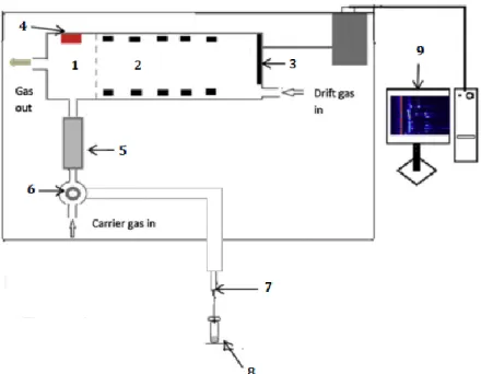
The spectrometer consists of a sample introduction system, a GC column, an ioniza-tion area, a drift tube and a detecioniza-tion area. The detector is an electrometer that measures the ion current as a function of time. Figure 5.2, illustrates the principal setup and inter-nal gasflow of the equipment.

Figure 5.2 - Schematic of the internal gasflow and the composing elements of the GC-IMS device

[64].

The sample is introduced into the device at the sample port. If the 6-Port-Valve (V) is at the default position, the gas sample will move through the loop by the action of the pump P and be redirected to the sample out socket. In addition, the carrier gas will be flushing the GC column and, both the carrier and the drift gases will leave the device at the gas out socket. At the second position of the valve, the carrier gas transports the sample into the GC column. The sample is then directed to the ionization region of the device. Here the sample molecules are ionized by an ionization source, which in the case of this device is a radioactive tritium source, with β-emission.

After ionization, the product ions, resulting from the ionization of the molecules in the sample are injected into the drift region through an ion-molecule injection shutter. The drift region, whose length is 9.8 cm, has several metal rings in order to maintain a homogeneous electric field gradient. The maintenance of a homogeneous field is im-portant since any irregularity in the field leads to a larger drift time or non-repeatable reads [69]. The potential difference between the ends of the drift region is of 5000 V.

Certain regions of the device, IMS region (T1) and the GC column (T2), the sample loop (T3) and the transfer lines (T4 and T5), are heated and can be changed for different application, such as for analysing different substances, and for cleaning processes.

The drift and carrier gases are controlled by electronic pressure control units, EPC1 and EPC2, respectively. These are the parameters, as well as the opening time of the valve and the percentage of the pump to fill or clean the loop, passible of being altered by the user.

In Table 5.1 the characteristics of all the materials used in this experiment are regis-tered.

Table 5.1 - List of the materials used during the course of this work, as well as their dimension

and their manufacturer

Materials Manufacturer

Ion Mobility Spectrometer coupled to a Gas Chromatography column (GC-IMS): 450 x 500 x 295 (WxDxH); 20 kg

G.A.S.® GmbH, Dortmund, Germany GC column: MXT-200, 30 m X 0,53 mm ID ---

Power Supply Adjustable DC power supply PS23023 _{0-30V/0-3A x 2Way 5V Fixed} Digital Thermometer and hygrometer ---

Digital Chronometer ---

Analogic Heatblock VWR®, Radnor, PA

Vials (20mL), with magnetic caps and

rub-ber seals VWR®, Radnor, PA

Teflon tube with female thread Bohlender GmbH, Grünsfeld, Germany _{Swagelok, Solon Ohio}

Sterile swab / cotton swab FL medical/---

5 mL syringes PIC Solution®, Pikdare S.r.l., Italy

21 G needles BDTM, Becton, Dickinson and Company,

Franklin Lakes, New Jersey

Petri dishes ---

Spectra

A GC-IMS chromatogram or spectrum is represented by the x-axis, the drift time, a y-axis, retention time and a colour scheme representing the signal intensity from the detector, z-axis. The x-axis has information regarding the drift time in milliseconds (ms) or relative to the RIP. The z-axis corresponds to the intensity obtained by the faraday plate as a voltage (V). Gas chromatography provides the y-axis information with the

30

column into the ionization region, a spectrum is plotted for a specific retention time. Each spectrum only requires 30 ms to be recorded [64]. The spectrometer may work in a positive or negative ionization mode of detection.

The chromatograms allow both a qualitative and a quantitative analyses where ana-lyte concentration is correlated with peak height and area [64].

To study the resulting data, the Laboratory Analytical Viewer (LAV) software is re-quired.

LAV software

The LAV software was developed by GAS and is used to visualize, both in 2D and 3D, and analyse the spectra produced by the GC-IMS equipment. Although the software has lots of functionalities, the most used ones were the standard and comparison Green/Red/Blue views, the Reporter and Gallery plugins and the Analytics functions. Figure 5.3 illustrates the main window of the LAV software. The standard view allows the visualization of the measured data in 2D, with the x-axis being the drift time, in mil-liseconds, and the y-axis the retention time, in seconds (Figure 5.3). The peaks’ intensity is displayed resorting to colour. The higher the intensity, the redder the peaks.

The comparison Green/Red/Blue view allows the comparison between a maxi-mum of three spectra. One of the three colours is attributed to a selected spectrum. If a new peak is present, it will be displayed by the colour attributed to the respective spec-trum. Figure 5.4 illustrates the comparison Green/Red/Blue view.

Figure 5.3 – Typical view of the LAV software. A spectrum of room air is shown in the standard

The first step in the spectra analysis is the definition of area sets. The area sets are defined by the user and enclose the peaks in the spectra. These area sets can then be compared throughout multiple spectra in the Gallery plugin of LAV to characterize and identify peaks. This feature provides the relative intensity of the peaks, which allows a much easier analysis. By exporting this data to an Excel sheet is possible to, automati-cally, obtain the peaks that show an intensity increase or decrease, from one spectra to the other. Figure 5.5 illustrates a part of the window of this plugin.

Figure 5.5 – Part of the window form the Gallery plugin. In this case, there are seven spectra being compared

for the identified area sets. The name of the area set is placed bellow each column. The red rectangle iden-tifies the functionality that provides the relative intensity of the area sets.

Figure 5.4 – Spectra with the Comparison Green/Red/Blue view. In this case, only two spectra were analysed. These are two spectra from room air. As can be observed, the peaks shared in both spectra present a yellow colour, while the non-shared ones present the colour attributed to their spectrum.

32

The characteristics of the peaks, such as retention time, drift time and intensity, RIP position and intensity can also be obtained in the Analytics tab, among other values. About the Reporter plugin, it places the chosen spectra side by side which allows a much easier comparison between spectra (Figure 5.6). In this plugin, spectra zoom in and zoom out is possible and retention times, drift times, intensity values and area sets can also be displayed.

Figure 5.6 – Window for the Reporter plugin. Two or more spectra can be compared in this view. Here, it is

possible to obtain the drift and retention times of the peaks and see if they coincide in the various spectra.

Preparation of the sample

In order to retrieve a bacterial sample from the culture, cotton swabs were used. The swabs were then placed into a 20 mL glass vial. The vial’s septum was perforated with two needles in order to make retrieving of the headspace possible. The sample was introduced into the device by means of a syringe or a Teflon tube depending on the experimental procedure followed.

In addition, a heat block, a chronometer, thermometers and a hygrometer to meas-ure room humidity in order to control the parameters of the measmeas-urement were used.

Previous protocol using MCC-IMS

Previous work has already been developed in the MCC-IMS equipment to deter-mine the measurement parameters that contribute to attain the best results [10]. These parameters are both related to the equipment and the treatment of the sample.

Parameters relating to the device include the drift and carrier gases flows, 500 mL/min and 25 mL/min, respectively, and the running time of the program, 10 minutes.

To obtain the sample, it was concluded that heating the swabbed bacteria at 40 ºC during 10 minutes, would provide the best results. To achieve sample headspace equilibrium 10 minutes are required, meaning that the released VOCs have reached a uniform dis-tribution inside the vial.

The pump of the device can be used to suck the headspace from the vial into the equipment.

The protocol used was as follows:

1. Gently roll the cotton swipe’s head back and forth on the bacterial culture pre-sent in the Petri dishes.

2. Cut the swipe’s head into a vial.

3. Close the vial and place it in the heat block.

4. Attach the Teflon tube from the sample port of the device to the vial. 5. Heat the vial at to 40 ºC during 10 minutes.

6. Run the measurement program.

Table 2 below contains the program previously developed.

Table 5.2 – Previously developed program used to perform the measurements.

Time (ms) V P R _(mL/min) Drift gas _gas(mL/min) Carrier

0 | 12% | 500 25

240 | | Rec | |

4160 Open 0% | | |

16200 Closed | | | |

600000 | | Stop | |

Optimization of the parameters

The previous developed protocol was followed in order to obtain the first meas-urements. Despite providing good results, the program could be improved for a better performance.

Since the chromatographic columns of the GC-IMS and the MCC-IMS are differ-ent, the drift and carrier gases flow had to be adjusted. For the drift gas flow the value chosen was 150 mL/min, not only because it was already used in other works of the group but also because previous calibrations were performed with the same value. The calibration is necessary to identify signals in the spectra.

34

that the majority of the compounds were present at the bottom of the spectra. A low flow was chosen at the start of the program to allow a better separation of these substances. The carrier flow started at 10 mL/min and was increased to 40 mL/min by the end of the program, allowing a short running time for each measurement.

Finally, the opening time of the valve was studied. As the valve controls the quan-tity of injected sample to be analysed, it is important that the majority of the sample enters the drift region for analysis. The sample loop has 1 mL. If the sample introduced at the sample port is less than the capacity of the loop, the rest will be filled with air. If, however, it is more, only 1ml will go through.

The valve was open for 10 seconds, which is equivalent to approximately 1.7 mL of headspace with the initial flow of 10 mL/min.

Figure 5.7 illustrates the effect of the carrier gas flow and the opening of the valve on the spectra. In the program of the Figure 5.7 a), the valve was opened for 4 seconds at an initial flow of 10 mL/min for the first minute. In Figure 5.7 b), the valve was opened for 10 seconds at the initial flow (10 mL) for the first 1 min 30 s

.

Figure 5.7 – Comparison between the spectra obtained in the GC-IMS equipment with different carrier gas

flows and valve opening time: a) carrier gas flow of 10 mL/min during 1 min and valve opening time of 4 seconds; b) carrier gas flow of 10 mL/min during the first 1min30s and valve opening time of 10 seconds.

As can be observed from the previous figure, the flow changes allow a much better resolution of the peaks.

Figure 5.8 – Program used in the GC-IMS to perform the measurements (BAC_PUMPTEST). The different

parameters are time (in milliseconds), drift and carrier gases flows (E1 and E2, respectively), pump (P), valve (V) and record (R).

The time is in milliseconds. R represents the recording of the data and V1 is the valve. Once these variables are set to 1, the recording is on and the valve opened. If set to 0, the data is not being recorded and the valve is closed. The E1 and E2 are equivalent to EPC1 and EPC2, which control the flow of the drift and carrier gases, respectively. P1 represents the percentage activated of the pump. In this case 20 %. Once again, if P1 is 0, the pump is turned off. Turning the pump on after the valve is turned off does not affect the data in any way since the connection with the sample inlet is cut off once the valve is closed. This is very useful since it helps to clean the sample loop during the running of the program.

Experimental procedure

As mentioned before, the first spectra were obtained using a previously developed protocol. However, since the GC-IMS is more sensible to VOCs’ than the MCC-IMS, it was hypothesised that there would be enough VOCs in the headspace at room temper-ature retrieved from the vial to obtain good results of bacterial samples. A measurement for one vial was made at room temperature, followed by a measurement after the same vial heated to 40 ºC.

The experimental procedure used was as follows:

1. Gently roll the cotton swipe’s head back and forth on the bacterial culture. 2. Cut the swipe’s head into a vial.