Risk aversion in financial crises

Risk Aversion in Financial Crises

Gonçalo Cunha

LUMS (Student No. 30687826); Católica-Lisbon (Student No. 152111056)

Advisor: Joni Kokkonen

Dissertation submitted in partial fulfilment of requirements for the degree of MSc in Business Administration, at Católica-Lisbon School of Business and Economics, 16th September 2013.

3 Abstract

This study is designed to understand how investors risk preferences change, when faced by financial crisis. Option prices implied densities provide information about market movements and risk preferences. The data used are European call options prices on the DJIA with a time to maturity of four weeks. This paper obtains the risk aversion estimates by the extraction of options implied risk neutral densities and their translation to real world densities, applied to three crisis : Dotcom bubble in 2001; Subprime mortgage in 2008 and European sovereign debt in 2011. RND is achieved by the use of two parametric methods: mixture of lognormal densities (MLN); and generalised beta distribution of the second kind (GB2). The risk transformation procedure from RND to RWD (real world densities) is achieved by applying the power utility function. The RND empirical results imply that the GB2 method is disregarded due to inferior quality whilst the MLN produces results of higher uncertainty and expected future results of index levels corrected downward. The risk aversion estimates obtained from the RWD generation process do not present any evident pattern of evolution from a stable financial period to one of financial shock. It is also important to mention that for some periods the risk aversion reached negative values. This is a surprising result due to existent theoretical assumption of positive risk aversion. Overall, this study documents inconclusive results. Nevertheless, several important topics are left for future research. Interesting developments would consist: either replicating this study considering more expiration dates, bearing in mind that too many periods would imply an extremely generalised risk aversion estimate that would be counterproductive for achieving the objective of this paper; apply another method from the available literature; or testing the negative estimates with more sophisticated models that are beyond the focus of this paper.

Key words: Risk Neutral Distribution, Real World Density, Mixture of Lognormal, Generalised

4 Table of Contents

I List of Figures ... 5

II List of Tables... 5

III Notations and Abbreviations ... 5

1. Introduction ... 6

2. Literature Review ... 7

2.1 RND Extraction Methodologies ... 7

2.1.2 Parametric Methods ... 8

2.1.3 Non-Parametric Methods ... 12

2.2 Risk Aversion Recovery Methodologies ... 13

2.2.1 Utility Function based Transformation ... 13

2.2.2 Calibration Function based Transformation ... 14

2.2.3 Parameter Estimation and Accuracy Testing ... 15

3. Data and Methodologies used... 15

3.1 Data ... 15

3.2 Methodologies used ... 16

3.2.1 RND Methodology ... 16

3.2.2 RA Methodology ... 18

4. Empirical results ... 20

4.1 Risk neutral densities... 20

4.2 Risk aversion measure and real world densities ... 23

5. Conclusion ... 28

IV References List ... 30

5

I List of Figures

Figure 1. Risk Neutral Densities estimates ... 21

Figure 2. Dow Jones returns from January 2000 to January 2013... 24

Figure 3. Real World Densities estimates... 25

II List of Tables

Table 2 Summary statistics of Mixture Lognormal densities for Risk Neutral Densities ... 22

Table 3 Estimate of the risk aversion parameter... 24

Table 4 Evolution of accumulated risk aversion parameters ... 27

III Notations and Abbreviations

GB2 Generalised distribution of the second kind GBM Geometric Brownian Motion

i.e. That is

MLN Mixture of lognormal RND Risk neutral density RRA Relative risk aversion RWD Real world density

6

1. Introduction

The purpose of this dissertation is to assess the impact of different crisis on investors’ preferences. In order to achieve this goal, this research focuses on how the aggregated risk aversion (i.e. how market participants behave towards uncertainty) evolves during financially troubling periods and understand if there is a specific pattern formation. This research comprises the last decade’s most troubling financial crisis: the dotcom bubble in 2000, the subprime mortgage crisis in 2008 and the European sovereign debt crisis in 2011.

The process to accomplish this investigation requires the extraction of risk neutral densities of a meaningful index option market and its transformation into real world density. The rationale behind the option prices implied densities is the following: option prices contain information about investors’ future expectations on the underlying asset. More specifically, an option price, with a matching exercise price, represents the opinion of one investor about the outcome of the underlying asset at expiration date. Several option prices of a given underlying asset are different opinions of different market agents. When aggregated, they compile a set of weights of numerous outcomes that determine the terminal price of the underlying asset from the perspective of the representative risk neutral agent. Furthermore, by transforming the risk neutral density into real world density it is possible to obtain the risk aversion estimates.

In this research, the considered option market index is the Dow Jones Industrial Average. Additionally, two parametric methods were selected to extract the risk neutral densities: mixture of lognormal densities and the generalised beta distribution of the second kind. In order to obtain the risk aversion estimates it was necessary to build the real world distribution, by applying a power utility function for the representative investor.

According to Bliss and Panigirtzoglou (2004), intuitively, the expected conclusion would be to perceive a countercyclical risk aversion pattern. In other words, in response to market crashes the average investor, for a certain risky asset, would require higher returns when compared to an economic expansion period. The aggregate risk aversion would increase as a consequence of recession and drop during growth. The resulting risk aversion estimates are fully explained in the empirical results analysis section.

The probability distributions’ forecast ability is the main reason why, many scholars decided to focus on this area of research: Taylor, (2005); Bliss and Panigirtzoglou (2004); Shackleton, et al. (2010); Jackwerth (2004).

The next section provides a brief review of the available literature on extracting both risk neutral and real world densities from option prices, section 3 describes the data and methodology used, section 4 describes the obtained results, and Section 5 concludes.

7

2. Literature Review

This section presents the basic concepts of risk neutral and real world distributions together with a non-exhaustive explanation of the main extraction methods for the two types of densities. The main objective is to understand which methodologies apply best to the execution of this research.

The Risk Neutral Density (hereinafter “RND”) of an index option market provides a distribution of probabilities for the Index’s future prices at the maturity of the option. These probabilities are a reflection of the market uncertainty perceived by investors. One can build such a density function due to the fact that each strike price (with the same expiration date) of a specific index option, offers information on investors’ expectation about future market fragility and instability levels (Bahra, 1997).

The risk neutral distribution is only equal to the real world density if investors have no specific reaction towards risk (risk neutral). As in reality this assumption does not hold, option prices will only incorporate the true beliefs about the future if a risk aversion measure is considered. With the corresponding coefficient of risk aversion, one may proceed with the forecasting activities (Bahra, 1997).

“In summary, risk neutral probabilities in conjunction with actual probabilities tellus about implied utility functions and thus about the economy wide preferences that investors exhibit. This information provides a fascinating look at the economy” (Jackwerth, 2004:64).

2.1 RND Extraction Methodologies

The multitude of methods can be structured into two categories: parametric and non-parametric. Both aim to generate models flexible enough to capture and explain the observed option prices.

Parametric methods are highly restrictive procedures as they rely on a large number of assumptions to generate data. Due to their structured nature, the mathematic process is relatively easy since there are few parameters to estimate. The inherent problem of these techniques is that since there are so many assumptions that in case the model specification is not a perfect match with the option prices (probability distribution not sufficiently flexible to fit observed option prices) the results will be very misleading (Bondarenko, 2003).

In contrast, the small number of assumptions and the many parameters that characterise the models produced by Non-Parametric methods allow an added flexibility that guarantees a superior fit of option prices. However, there is an implied cost to this extra generality. As models are too elastic and adjust to all the available information, they become exposed to market noise and individual options anomalies, causing overfitting and distorted results. It is also a complex and slow computing procedure (Jackwerth, 2004).

8 2.1.2 Parametric Methods

From the available literature it is possible to allocate the Parametric methods in three main streams for RND extraction: The first approach specifies a distribution form for the RND and compares the differences between the generated option prices and the observed option prices; the second requires defining an option pricing function and extracting the risk neutral density based on the Breeden and Litzenberger (1978) model; and the last type of extraction has a longer procedure by assuming a specific relation between implied volatility and strike prices and then applying the Breeden and Litzenberger (1978) model to the indirectly interpolated call pricing function in order to obtain the RND (Jackwerth, 1999).

Regarding the form assumption based methods: consists in defining a parametric assumption about the RND form. There are several ways to achieve this goal: (i) mixture methods create a potential RND function from a weighted average of several simple probability distributions, adding great flexibility to fit the option prices. (ii) expansion methods, as the name implies, expand elementary distributions by adding correction terms in order to control higher moments, improving their flexibility. (iii) generalized distribution methods use several distribution functions with parameters that go beyond the typical mean and volatility of normal and lognormal distributions, as limiting cases.

Lognormal mixture, first suggested by Ritchey (1990), is the most commonly used method within the mixture category. It is a weighted combination of two lognormal distributions, allowing a large variety of flexible shapes due to the extra three parameters ( ), (explained thoroughly in the methodology section) when compared to the single lognormal density. Once the probability density is established according to the form assumption, the option prices are then used to estimate the true parameters of the distribution. This process requires the application of the least square method between the generated option prices (with Black and Scholes (1973) option pricing formula as foundation) and the market option prices. The parameters that yield the lowest difference value will form the true risk neutral density of the underlying asset.

There can be mixtures with three lognormal densities or more. Melick and Thomas (1997) use a mixture of three lognormal applied to American options on crude oil futures, during the Persian Gulf crisis, finding that the result of the estimated distributions were “consistent with the market commentary at the time” (Melick and Thomas, 1997, p. 92) and that it outperformed the simple lognormal assumption. However, the more lognormal distributions are added, the higher the number of parameters, which in turn creates tedious calculations procedures and is less interesting for the traditional options that are traded across a low range of strike prices (Bahra, 1997).

In summary, the two lognormal mixture is quite appealing for researches which start with little information about the stochastic process of the options market. It is a method easy to implement and assures non-negative distributions (Bahra, 1997). Being directly linked to the Black and Scholes (1973) is just another evidence of its simplicity (Cont, 1997). However, according to some authors there are some inherent disadvantages: yields too thin tails, which may create some difficulties in capturing higher statistical moments (Cont, 1997); there is no

9 theoretical background to assume that index option prices should follow such a distribution (Cont, 1997); is prone to overfitting when the number of distributions equals three or more (Jackwerth, 2004), and may return a bimodal density creating confusing analysis (Taylor, 2005). Regarding the second type of form assumption based methods, the expansion methods, are techniques built on the rationale that the Black and Scholes assumption about price dynamics (Geometric Brownian Motion) is unreliable. Therefore, these methods add to Black and Scholes (1973) natural risk neutral density (lognormal) a second term, the expansion measure. This term is considered as successive corrections to the original RND, providing more flexibility by permitting control over the parameters that correspond to skewness and kurtosis (Jarrow & Rudd, 1982). In a similar procedure to the mixture methods, from the new function (lognormal plus adjustments), a preliminary distribution is created, allowing the estimation of the parameters with help of the observed option prices, creating the final RND that represents the future density of the underlying security (Cont, 1997).

Edgeworth series expansion (Jarrow & Rudd, 1982) is a good example of an expansion method. It is theoretically similar to the Taylor expansion (a function can be expressed by an approximated simpler polynomial), though instead of simplifying a function, this expansion is used to generate a more complicated RND in order to capture deviations from log-normality (Jondeau & Rockinger, 2000).

Lognormal-Polynomial Density Functions or Hermite Polynomial, an alternative expansion method, was developed by Madan and Milne (1994). It assumes that standardized returns have a standard normal density multiplied by a polynomial function. Therefore the density of prices is a lognormal density multiplied by a polynomial function. In other words, they obtain the RND through a multiplicative perturbation of the simple lognormal density in order to allow a certain control of higher moments (Taylor, 2005).

Both Hermite and Edgeworth expansion methods yield similar RND results when applied to exchange rate options (Jondeau & Rockinger, 2000). Even though they have a strong theoretical foundation, there is no guarantee that the generated densities will be strictly positive (Jackwerth, 2004). Additionally, when compared to the mixture of lognormal technique they present inferior abilities in capturing skewness (Jondeau & Rockinger, 2000), an essential statistical moment to capture the right movements of the underlying asset.

The final category of the form based assumption methods is the generalised distribution methods. These type of methods use density functions which include higher statistical moments, more specifically skewness and kurtosis. GB2, the Generalised Beta of the second kind, is a well-known generalised distribution method, developed by Bookstaber and McDonald (1987), which gives origin to several other generalised methods. It is an extremely flexible method, due to the enclosure of a large number of known distributions as special or limiting cases (e.g. Log t, log Cauchy, gamma, exponential, lognormal), therefore allowing to change shapes drastically according to different combinations of parameters as it can roam across the included distributions limits.

10 GB2’s density function depends on four parameters ( )with no specific theoretical meaning. The parameters work interactively in determining the shape of the distribution. The great flexibility in shape creation permits large higher moments (skewness and kurtosis). Even though the four parameters have no theoretical meaning, some parameters have a specific role in the RND construction, for example: is a scale parameter, having an ovious role in defining the height of the distribution; the product of controls the fatness of the distribution (Bookstaber and McDonald, 1987). The density’s parameters are easy to estimate, the method allows a high degree of flexibility, a non-negative density is assured, it does not involve subjective choices, and the RND can be easily transformed into real world density. The main disadvantage is the lack of theoretical meaning of the parameters, which may cause some difficulties on defining the initial inputs for the estimation process (Taylor, 2005). According to Taylor’s book on Price Dynamics (2005), GB2 is the only method that fulfils the necessary conditions to be a perfect RND generator: Positive densities are assured, allows general levels of the third and fourth moments; provides fatter tails than the single lognormal; there are analytic formulae for the density and the call price formula; discrete option prices do not affect results; easy parameter estimation; estimation does not require subjective choices; and the RND can easily be transformed into RWD.

Moving to a different style of parametric methods, the price assumption based methods, are an RND extraction type which requires the specification of an option pricing function and the use of the Breeden and Litzenberger (1978) formula, which shows that the RND function can be learnt by the second derivative of the European call option pricing function with respect to the strike price. The simplest method of this group is based on the Black and Scholes (1973) pricing formula, which assumes that the underlying asset price follows a Geometric Brownian Motion (“GBM”) stochastic process. Based on this assumption, replacing the expected return of the underlying asset (µ) by the risk free rate , and by applying the Breeden and Litzenberger (1978) model, their formula yields a lognormal RND function. Although the Black and Scholes assumption about price dynamics (GBM) (i.e. constant expected drift rate and constant volatility) is quite different from reality (Rubinstein, 1985), this pricing formula serves as basis for other methods that assume different stochastic processes for the underlying security price dynamics other than the GBM.

Heston’s (1993) model assumes a mean-reverting stochastic volatility process for the underlying price and presents a closed form solution for the implied RND. One of its main features is the ability to capture the speed by which the market volatility reverts back to normal. The generated option pricing formula has 5 parameters ( √ √ )1 _{to be}

estimated, and by using the Breeden and Litzenberger (1978) second derivative the RND can be inferred. In contrast to the simple GBM, this method displays plausible smile effects (i.e. implied volatilities plotted across strike prices) (Shackleton, et al., 2010). However, according to Jondeau and Rockinger (2000), it is a slow procedure as it implies high computational cost,

1

Where captures the speed by which volatility is mean reverting; √ represents the long run volatility; is the volatility of volatility; correlation between the two implied Brownian motions; and √ the measure of instantaneous volatility.

11 and also it has difficulties in capturing skewness when compared to a mixture of two lognormal or expansion methods.

Jump Diffusion process is another alternative for a stochastic based method that assumes price dynamics process as lognormal jump diffusion, which equals to a GBM plus a Poisson jump process. This method, usually applied to exchange rates (e.g. Malz,1995b or Jondeau and Rockinger, 2000), shows the likelihood of a possible jump on exchange rates based on investors’ perception. It derives a closed form solution for the terminal RND function corresponding to a mixture of two lognormal densities. According to Jondeau and Rockinger (2000) models comparison research, the Jump Diffusion model is the top performer for exchange rate options with long term maturities.

Just as the previous type of methods (price assumption based), this group of techniques, implied volatility assumption based methods, define their RND extraction strategy based on the Black and Scholes failure: As previously mentioned, Black and Scholes (1973) assume a GBM for stochastic process and a single volatility for all the strike prices of the underlying asset, with the same expiration. As consequence, the implied RND is a simple lognormal distribution. By calculating the implied volatility based on option market prices, one can understand that each option with a certain strike price has a different implied volatility, which means that Black and Scholes assumptions are quite different from reality. By plotting the implied volatilities across strike prices, it is possible to perceive a “U” shape, called smile, as opposed to a flat line caused by the constant volatility of the Black and Scholes assumption (Bahra, 1997).

Based on this reasoning, the implied volatility based methods interpolate the implied Black and Scholes volatility smile, defining a specific relation between the implied volatility and the strike price. This approach was suggested by Shimko (1993), assuming the implied volatility function as quadratic. Just as the flat smile corresponds to a lognormal RND, this implied volatility function reflects a certain form of RND with a higher degree of flexibility and better related to the market movements. Using the “Black and Scholes as a translation device” (Bahra, 1997:18), an indirectly interpolated call pricing function is generated. By applying the Breeden and Litzenberger (1978) formula to the pricing function, the RND can be obtained (Andersen & Wagener, 2002). The main drawback of Shimko’s approach is the fact that the distribution generated lacks smoothness in the tails area, therefore Shimko inserts lognormal tails, which are considered as unable to properly capture higher moments. Bahra (1997) criticises Shimko’s method, saying that: the quadratic assumption may be too restrictive; and that the lognormal tails is a fragile solution for the lack of smoothness at the both ends of the distribution. Bahra (1997) suggests the cubic spline (i.e. polynomial function that can be based on a simple form locally but, be globally flexible and smooth) as the best possible assumption for this approach, although this solution is considered as a non-parametric approach. In general, these methods have few parameters to estimate, however they may yield negative densities or smoothness problems, but the main drawback is that the function selection procedure may seem arbitrary. Other implied volatility functions may be linear, hyperbolic, parabolic and polynomial.

12 2.1.3 Non-Parametric Methods

There are several types of Non-Parametric RND extraction techniques. They can be divided into three man groups (i) flexible discrete distributions obtain flexible shapes by adopting the least number of constraints, (ii) kernel regression methods, which consist of defining a non-parametric function to fit the observed option prices, (iii) maximum entropy methods, fit a non-parametric probability distribution to explain the data.

Flexible discrete distribution is a class of methods which includes two types of approaches: one uses a general equation to approximate a function of implied volatilities (the cubic spline applied to Shimko’s method as explained above) and a second one that estimates the RND directly with a general function. For the second type, according to Rubinstein (1994) it must be assumed that each stock price has a certain probability of occurrence. These probabilities, assuming a set of basic restrictions, compose the RND. Then a fixed difference between the different stock prices is assumed (Δ). In consequence, probabilities become proportional to the price of a butterfly spread. These probabilities are then considered as parameters to be estimated. The parameters can be estimated by minimising the difference between observed and fitted option prices. According to Jackwerth and Rubinstein (1996) this function must incorporate a smoothness factor in order to provide probabilities closer to reality. It is important to mention that the minimisation procedure has a trade-off, as the lower the difference the lower the smoothness (Taylor, 2005). Both flexible discrete methods can generate flexible shapes, though they do not guarantee non-negative densities and imply long and complex calculations. It has been verified that for the FTSE100, densities estimated by spline methods have an inferior fit with the market option prices than the mixture of lognormal and the GB2 (Liu, et al., 2007).

The kernel regression method is based on Ait- Sahalia and Lo (1995) finding that the Breeden and Litzenberger (1978) second derivative could also be applied in a discrete way, given a large enough information set (Cont, 1997). This class of methods is related to nonlinear regressions. However, instead of defining the form of the linear regression, the general logic is the following: each implied volatility, with a certain strike price, is a data point on the “smile” where the true volatility function should cross. The kernel measures how likely the function will pass away from that point. The further away the function is, the less weight is attributed to the specific strike price that contributes to the RND composition. There is an extra factor, the bandwidth, which controls the trade-off between smoothness of the kernel regression and fitting the data (Jackwerth, 2004). The densities obtained by Ait- Sahalia and Lo (1995), when applying this method to S&P future options, are constantly different from the erroneous single lognormal and present significant kurtosis and skewness (Cont, 1997). The drawback of this method is that it tends to be a complex and very data-intensive process (Cont, 1997). It requires large datasets and is unsuitable for data that presents large gaps between strike prices (Jackwerth, 2004).

The maximum entropy method defines a prior distribution to find the risk neutral density that best fits the option prices, based on a special feature. This feature consists in assuming the least possible information about the prior distribution. It possesses solely the most basic constraints: positive probabilities that sum to one (Jackwerth, 2004) and that the set of option

13 prices are exactly represented by the theoretical option price formula. The inexistence of smoothness constraints has its disadvantages as it may yield multimodal densities (Cont, 1997).

2.2 Risk Aversion Recovery Methodologies

Option prices provide insightful information about the future probability density of the underlying asset. However, since densities directly estimated from market option prices are proven to be risk neutral, due to the underlying assumption of risk neutrality of market participants, it is not possible to produce accurate forecasts (Bliss and Panigirtzoglou, 2004). In other words, as RNDs do not incorporate market participants risk aversion, or behaviour towards assets’ risk premium (i.e. the compensation investors require by tolerating excess risk in comparison to the risk free rate) they cannot be used as a reliable forecaster of market expectations (Anagnou et al.,2002). This is how the necessity of estimating densities that are able to include investors’ risk aversion (real world distributions) arises.

There are three main streams of how to recover the real world density function. The first thread is based on a risk transformation rationale that can be divided in (i) assuming a utility function for a representative agent that converts the artificial risk neutral density into real world density, or (ii) calibrating the RND to obtain the RWD. The second thread calculates the RWD from an historical time series of asset prices, which according to several scholars, such as: Shackleton, et al. (2010); Liu, et al. (2007), contrasts significantly from densities extracted from option prices. And finally the third thread, a more complex methodology, jointly uses both asset and option prices to estimate the relation between the RND and the RWD which encloses the risk premium and jump risks (Liu et al., 2007).

From these three threads, this research considers only the first one: the risk transformation based methodologies which comprises the utility function methods and the calibration function methods. The second will be disregarded as throughout the available studies, it is possible to perceive that in general, results derived from option prices contain more information about the true densities than results estimated from historical time series of asset prices, with the exception of one day horizon estimates where they outrank option prices based densities (Shackleton, et al., 2010; Liu, et al., 2007). Although the third thread, the joint approach, has been proven to be a very satisfactory producer of RWD (Shackleton, et al., 2010) due to improvements for short term horizons, it will also be overlooked as it goes beyond the focus of this research.

2.2.1 Utility Function based Transformation

Under a certain set of assumptions, the risk neutral density can be mutated into the real world density by defining a risk preference function following Ait-Sahalia and Lo’s (2000) risk relation formulation. The utility function, is considered as the link between the RND and the risk adjusted density, embodying the representative agent behaviour towards risk, considered as the relative risk aversion measure (hereinafter “RRA”) (Bliss and Panigirtzoglou, 2004).

The main utility functions that define the representative agent’s risk aversion considered in the available are: (i) power utility function and (ii) the exponential utility function. Both functions

14 rely on the parameter γ. The power function has a constant relative risk aversion, therefore the RRA measure equals to the gamma (γ). On the other hand, exponential function is subject to a constant absolute risk aversion, which means the gamma parameter will vary according to the level of the index. The RRA measure for the latter utility function equals to γ (Bliss and Panigirtzoglou, 2004).

In order to build the actual density, the optimal parameter γ (i.e. the gamma which assures the best match between the real world density and the observed underlying asset prices), must be estimated. From the available literature there are two main methods to perform the optimisation procedure: Berkowitz LR3 test or the likelihood function maximisation that will be described in a following section. Once the adjusted densities are formed, their accuracy may be tested with the same evaluating methodologies.

According to Bliss and Panigirtzoglou (2004), adjusting the artificial risk neutral densities into real world densities through both utility functions provided for the majority of cases an accurate forecast of the future price distribution for the underlying index. Additionally, within Bliss and Panigirtzoglou’s data set (FTSE 100 and S&P500), there is evidence that the exponential utility function yields RWDs with slight better fit than the power function. However, assuming a power utility function is more convenient due to the constant RRA which generates simpler calculations. For this reason and in addition to the fact that both functions generate similar (average) RRA measures, the preferable utility function to be implemented as utility based risk transformation techniques, would be the power function.

2.2.2 Calibration Function based Transformation

Calibration transformation method is another approach, which belongs to the first thread mentioned in section 2.2, which allows the transformation of risk neutral densities into real world densities. “The objective of statistical calibration is to transform forecast densities to probability assessment methods that generate reliable forecasts statements” (Ivanova and Gutierrez, 2013), in other words, the principle of statistical calibration is based on guaranteeing consistency between the density forecasts and the observations (Gneiting, et al., 2007). The process is considered as tuning the risk neutral “scale” by applying a certain calibration function, obtaining a RWD. The most common calibration function used amongst the available literature is the cumulative density function of the Beta distribution, first suggested by Fackler and King (1990) while studying commodity option prices densities. While the utility based methods have only one parameter (gamma), this calibration function has two calibration parameters, j and k, which has the advantage of allowing extra flexibility. Nevertheless, according to Liu et al. (2007), even though the calibrated RWD provided a superior match with the observed option prices than the RWD based on utility function, the difference was not substantial, and since RWD has a more complex form for the calibration transformation, the utility function technique will be the type of transformation used in this research to obtain the representative risk aversion levels. More specifically, the power utility function for the reasons already mentioned.

15 2.2.3 Parameter Estimation and Accuracy Testing

Berkowitz LR3 (2001) and the maximum likelihood are the main methodologies to estimate the optimal parameters that will generate the RWD. The rationale behind both procedures is simply choosing the risk aversion parameter that yields the most robust RWD in terms of good fit.

Berkowitz (2001) developed an approach to evaluate the forecasting ability of option prices implied densities, the LR3 statistic. Besides this standard application, Bliss and Panigirtzoglou (2004), use this test to estimate the risk aversion parameter gamma. The rationale is the following: the gamma that generates the RWD with the most accurate forecast ability, is obviously the one that best represents the aggregate investors’ risk aversion level (choice of gamma is made by maximising the forecast ability of the RWD).

Just as the Berkowitz LR3 statistic, the likelihood function can be used to test the accuracy of the PDFs and estimate the transformation parameters. The parameters can be estimated by seeking the maximum log likelihood function. According to Liu et al. (2007), the LR3 statistic is a good method for testing the goodness of fit, however, in terms of parameter estimation the log likelihood maximisation is the preferred technique. This research will follow the same preference regarding parameter estimation.

3. Data and Methodologies used

To investigate the risk aversion behaviour before and after the burst of financial crises, risk neutral and real world densities are evaluated for European call option contracts on the Dow Jones Industrial Average Index (hereinafter “DJIA”), with a time to maturity of four weeks. This research studies the prices of options on DJIA for three periods. Each period corresponds to approximately 10 months before and 10 months after the peak of the studied crises: dotcom bubble, the subprime mortgage crisis and the European sovereign debt crisis. In other words, this paper considers two risk aversion estimates for each crisis: the first right before the financial stress event reaches its peak, and the second while the market is still exposed to the crisis effects. The full calendar range for each crisis is the following: from February 1999 to March 2001 for the dotcom bubble, August 2007 to August 2009 for the subprime mortgage crisis and May 2010 to September 2012 for the European sovereign debt crisis.

The reason for extracting options of 10 subsequent expiration dates for each analysed period, which correspond to the aforementioned 10 months, can be found in Bliss and Panigirtzoglou (2004) work on risk aversion estimation. They say that if focusing on single point estimates (recover the risk aversion from a single RND), the market degree of risk aversion would be too exposed to that period’s specific information. Therefore, by including 10 RNDs in the risk aversion recovery process, it is possible to avoid biased risk aversion estimates.

The considered moments of occurrence for each crisis, that split in two (before and after) each of the above mentioned periods, are easily situated: The burst of the online bubble occurred

16 after the Nasdaq Composite index achieved its peak on the 10th of March 2000; regarding the housing bubble, even though the economy entered a recession at the end of 2007, the main effects were felt across the world after the bankruptcy of Lehman Brothers on the 14th of September 2008. The European sovereign debt crisis is an exception, since it does not have an evident “burst”. Nonetheless, the date considered is August 2011 when more stable European countries were downgraded by the rating agencies and the European stock markets suffered heavy falls exposing the rest of the world to fears of an unsolved sovereign debt crisis.

According to the available literature, the most reliable option prices used are the average of the closing bid and ask quotation (Jondeau and Rockinger, 2000). To be able to compare different implied distributions, the analysed options must have the same time to maturity, which in this case for the DJIA four weeks options, they have the same expiry time: the third Saturday of every month. Together with the index dividend yield, the option quotations were extracted from the Wharton Research Data Services. Regarding the risk free rate, this paper uses the three month Euro interest rates obtained from Datastream.

Concerning the moneyness, too deep in the money options are characterised by high illiquidity. As considering these options could probably lead into generation of biased results (Andersen and Wagener, 2002), a filtering procedure is applied consisting in excluding options with bid below 0,125.

Summary statistics for the DOW Jones option data set for each of the analysed periods is presented in the Appendix. It includes the calendar range and number of filtered option prices for all expiration dates (10) considered in each pre and post burst periods for the three crises. It also identifies which expiration dates were considered as right before and right after the bursts, used for the single RND analysis.

3.2 Methodologies used

This succeeding subsection aims to explain the process undertaken to achieve the empirical results obtained in this dissertation.

Before introducing the applied density extraction methods it is important to mention that the meaning of the used symbols have the standard meaning in option valuation: is the call option price; is the option’s strike price; is the risk free rate; is the expiration date of the option; is the price of the underlying asset; and the risk neutral density and real world density are denominated as ( ) and ( ) respectively.

3.2.1 RND Methodology

Across the available literature there are different opinions regarding which method is the top performer. However, according to Jackwerth and Rubinstein (1996), given a large enough number of options, the RNDs produced from any reasonable methods tend to be rather similar. Hence, this paper will focus on both Mixture of Lognormal and GB2, mainly due to their straightforwardness and general relatively high performance: Taylor (2005); Liu, et al. (2007); Jondeau and Rockinger (2000); Bahra (1997).

17 The mixture of two lognormal densities method is a weighted average of two lognormal densities, that comprises five parameters ( ), two parameters for each of the lognormal distributions, one based on the underlying asset price ( ) and the other which defines the standard deviation ( ) of the distributions, and a fifth parameter ( ) which establishes the relative weight for each distribution. Denoting the single lognormal density function as:

( | )

√ [ [

( ) [ ( ) ( ) ]

√ ] ] (1)

The mixture of lognormal risk neutral density can be written as:

( ) ( | ) ( ) ( | ) (2) In order to estimate the parameters that allow the “mixture” to shape a curve that best fits the market option prices, it is necessary to minimise the squared errors of the difference between the observed option prices and the theoretical option prices. This theoretical option price can be achieved by the weighted average of the Black and Scholes (1973) call option prices of each of the lognormal densities, with their respective parameters:

( | ) ( ) ( ) ( ) (3) The optimal minimisation, which yields the best parameters, can be reached by using the least square methodology:

( ) ∑ ( ( ) ( | )) (4)

Solver is the mathematical tool from Excel used to minimise the function ( ) to estimate the optimal parameters.

The generalised beta of the second kind method (GB2) is described by four positive parameters ( ) which allow a great flexibility in shape creation due to a large variety of different combinations for the four statistical moments. The GB2 density function can be described as:

( | ) _{( )}

[ ( ) ] (5)

The function included in the density function is defined by the following terms of the gamma function:

( ) ( ) ( )

( ) (6)

18 ( ) ( )

( ) (7)

From formula (7), it is possible to conclude that can be obtained by: ( ) ( )

( ) (8)

Therefore, the parameters a, p and q can free roam while b is derived from the previous formula. Once this constraint is guaranteed, it is possible to assume that the theoretical option prices depend on the cumulative distribution function of the GB2 ( ), which in turn can be

explained by the cumulative distribution function of the denoted as incomplete function:

( | ) ( ( )| ) (9)

With defined by the following function:

( ) _{( )}( ) (10)

Given that the density is risk neutral and that the parameter b is derived from a, p, q and S, the theoretical call option price can be written as:

( ) _{[ ( ( )| )] [ ( ( )| )] (11)}

Once it becomes possible to compare the market option prices and the obtained option prices, the four parameters ( ), that generate the density curve closest reality, can then be estimated by minimising the function ( ), defined in equation (4).

3.2.2 RA Methodology

Regarding the risk aversion recovery process, this research uses a parametric risk transformation method which follows Bliss and Panigirtzoglou (2004) power utility function. Their research focuses on estimating the representative agent’s relative risk aversion by adjusting the risk neutral densities, with the utility fucntion, and deriving the real world densities.

Bliss and Panigirtzoglou (2004) work, is based on Ait-Sahalia and Lo’s (2000) formula that identifies the relation between RND ( ( )) and RWD ( ( )) by a representative investor’s utility function ( ( )):

( )

( )

( )

( )

( )

With as a constant and the function ( ) the pricing kernel, the quantity proportional to the marginal rate of substitution between the risk neutral density function and the real world

19 density function (Ait-Sahalia and Lo, 2000), in other words it is the theoretical relationship between RND, the RWD and the risk aversion function.

Bliss and Panigirtzoglou (2004) define the power utility function as:

( )

(13)

The implied RRA, measure of the degree of risk aversion, for this specific utility function is constant and equal to the gamma parameter:

_{( )}( ) (14)

Once the utility function is defined, it becomes possible to estimate the real world density function, solving the presented equation (12) for ( ):

( )

( ) ( ) ∫ ( ) _{( )}

(15)

The denominator results in a constant value, which is a necessary term to guarantee that the density function is normalised and integrates to 1, with simply different from .

Applying formula (15) to the mixture of lognormal risk neutral density function, the real world density function can be obtained with the following formula:

( ) ( | ) ( ) ( | ) (16) With and defined as:

(

)

₍₁₈₎

The risk aversion measure (gamma) is then selected in a way which allows the combination of real world parameters ( ) that maximise the log likelihood function, which can be written as:

( ( | )) ∑ ( ( | ))

(19)

As it is possible to understand from the formula, several RND vectors ( ) and their respective observed price of the underlying asset from different periods are also taken into account. The main reason is to avoid specific period information to disturb the risk aversion estimate and therefore misleading the RWD parameters selection process.

20 The maximisation is achieved when the gamma generates a set of RWD parameters ( ) that guarantees the best match between the observed prices and the real world density. Therefore the selected gamma is the optimal measure of risk aversion.

4. Empirical results

This section will present the results obtained from both risk neutral and real world densities estimations for the three crises considered. The first part will compare and select which RND recovery method is considered as more robust, followed by an illustration of how the RND densities change with the manifestation of financially stressful events. And finally, the main object of this research, to study the possible changes in the representative agent’s risk aversion, in financially stable periods and in financial crisis’ periods.

4.1 Risk neutral densities

The table below shows the results of the minimisation of the sum of squared errors ( ( ))that select the best possible parameters that generated the closest fit of the density curve to the market option prices.

Table 1

Minimum of G(θ) function - sum of squared errors - for each of the RND extraction methods for the periods pre and post crises.

Method Dotcom Subprime Sovereign

Before After Before After Before After

MLN 0,062 0,157 6,935 0,307 0,475 0,223

GB2 0,099 1,741 6,941 0,439 1,003 0,282

Table 1

Table 1 implies a superior performance for the mixture of lognormal method in fitting the observed prices in every single period. This higher ability of the MLN to capture the behaviour of the option prices is more evident for both periods of the dotcom crisis and for the pre sovereign debt crisis period. It is also possible to assume that the extremely high value of the function for the generated density of before the housing bubble in 2008, may be due to the timing selection of crisis peak (Lehman Brothers bankruptcy). The period before the dotcom crisis yields the lowest minimisation values.

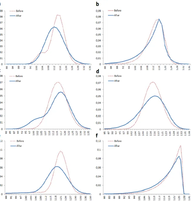
21 Figure 1. (a) RND obtained from mixture of lognormal method for before and after of the dotcom bubble burst. (b) RND obtained from GB2 method for before and after the dotcom bubble burst. (c) RND obtained from mixture of lognormal method for before and after the subprime mortgage crisis. (d) RND obtained from GB2 method for before and after the subprime mortgage crisis. RND obtained from mixture of lognormal method for before and after the sovereign debt crisis. RND obtained from GB2 method for the sovereign debt crisis.

By analysing the implied densities from the Dow Jones option prices, it should be possible to measure market participants’ perceptions of both market uncertainty and risks towards future market performance. Therefore we should expect some major differences between the pre crisis stage and the after burst period. As it is possible to see from Figure 1, risk neutral densities formed by the GB2 method, do not demonstrate to be able to measure investors’ expectations about market’s uncertainty as for both periods, they do not present a strong difference between the pre and post phases for each crisis, with the exception of the 2008 stress event which shows a larger width (higher uncertainty) for after the bubble burst. The MLN curves, on the other hand, provide relevant differences and shall be examined in detail.

22 Overall, it is possible to conclude that even though the subprime mortgage crisis in 2008 of the GB2 yield a ( ) almost as low as in the MLN, given that both online bubble analysed periods and the phase before of the European debt crisis demonstrate a big gap of fitting robustness, added to the fact that the RND GB2 graphs do not show significant differences in curve characteristics before and after each crisis, this research will solely focus on the mixture of lognormal method.

As mentioned, the MLN risk neutral densities show considerable differences when comparing pre and post crises periods. These differences reflect the new information obtained by investors changing negatively their expectations about the month after the burst of each crisis, not taking into account any measure of risk aversion. Even though the fit varies from density to density, it is possible to perceive a trend from pre crisis period to post crisis, a movement of the probability masses to the left together with an expansion of the width of the densities. In other words, there is a general rise of uncertainty with a great number of market participants expecting lower index levels, which indicates an increased anxiety among investors for the future index level.

Table 2

Summary statistics of the mixture of lognormal risk neutral densities for the six analysed periods.

Statistics Dotcom Subprime Sovereign

Before After Before After Before After

Mean 113,21 112,68 115,44 114,32 119,89 118,19

Standard Deviation 5,76 6,25 5,69 8,29 6,59 7,67

Kurtosis 0,22 0,25 5,56 -0,05 8,88 1,93

Skewness -0,63 0,09 -0,18 -0,49 -2,05 -0,87

Table 2

Table 2 presents a range of summer statistics that will be carefully analysed, in order to better understand information contained by the MLN risk neutral densities and their specific changes caused by the burst of each crisis.

From the values available on Table 2, it is possible to observe a substantial increase of the standard deviation (the measure of uncertainty around the mean) and the general fall of the mean (the expected value of the index), after the burst of each crisis, changes which confirm the aforementioned trend. However, in terms of the distribution of the probability masses, given by third and fourth statistical moments, each crisis has a specific combination of changes.

Regarding these higher statistical moments it is important to know that kurtosis measures the probability that investors attach to extreme outcomes. High kurtosis would result from more likely extreme outcomes, or “fatter” tails. Skewness characterises the asymmetry of the density function. In case the implied density is positively skewed, this means that the right tail is longer than the left, however there is less probability attached to outcomes above the mean. In more practical terms positive skewness indicates that there is a strong probability of the

23 underlying asset price to be below the mean, however, there is a remote possibility of having extremely positive results (Syrdal, 2002).

For the online bubble, the kurtosis measure slightly increases, which shows that investors attach a slightly higher likelihood to extreme outcomes which may be a source for the added volatility. Skewness levels show that after the bubble burst, a large amount of probability mass moved from the right of the mean to the left, building a longer right tail. This means that after the crisis the density became positively skewed (longer right tail, but larger portion of probability mass on the left side of the distribution), which shows that more market participants expect the prices to be relatively below the expected index price. Nonetheless, the longer right tail indicates that a few investors also expect extreme positive outcomes, probably based on the thought that crises may generate new opportunities.

Regarding the mortgage subprime crisis, there is a lower level kurtosis after the crisis and increase of skewness to the right. These results might indicate that the investors are aware of the pessimistic situations and do not expect an even worse development of the index, nor any sudden improvements (absence of extreme values). According to the higher negative skewness, the majority of market participants do not believe that the index can undergo slight negative changes, while a small number of some investors expect extreme negative outcomes. After the peak of the European sovereign debt crisis, common expectation regarding the index price moved to the left as skewness level became less negative. At the same time there are lower expectations towards extreme outcomes. Even though the uncertainty increased and the future prices are expected to be lower, from the summary statistics, it seems as the investors do not expect any dramatic changes.

To conclude, the third and fourth moments did not present the expected evolution: higher kurtosis (ECB, 2011) and more negative skewness during the financially troubled periods (Dennis and Mayhew, 2002). However, characteristics such as increase of uncertainty and movement of the expected index level to the left were clear evidences that the risk neutral distributions could detect some of the effects crises impose to the financial markets.

4.2 Risk aversion measure and real world densities

By specifying a power utility function for the market’s representative investor, based on a set of RNDs, it is possible to estimate the market’s degree of risk aversion for each period analysed. Intuition, would suggest that the representative investor would become more risk averse as risk increases (Bliss and Panigirtzoglou, 2004).

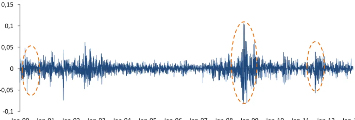
24 Figure 2. Dow Jones Industrial Average Index returns from January 2000 to January 2013.

This figure shows Dow Jones Industrial Average Index returns over the past decade. Volatility, as easily observed, has not been constant over time, and the three dashed areas which highlight the periods post burst, present clear signs of higher volatility. Therefore it would be expectable that during these unstable periods, it would be possible to observe a higher risk aversion measure (γ) than the respective pre crisis phase.

The risk aversion estimates, calculated with the maximisation process given in formula (19), are shown in table 3. From the presented values, it is possible to conclude that at least for the subprime mortgage and sovereign debt crises the gammas actually increase. However, both housing and online bubbles exhibit some negative risk aversion parameters, which is inconsistent with the usual assumptions of positive risk aversion.

Table 3

Estimate of the risk aversion parameter γ.

Dotcom Subprime Sovereign

Before After Before After Before After

1,44 -0,14 -6,36 -0,19 5,13 5,51

Table 3

When studying the evolution of the risk aversion estimates from the more peaceful period to the highly unstable period that characterise the majority of crisis, one can perceive different paths. The dotcom bubble the most unexpected results: fall of risk aversion after the burst until a negative levels, even if close to zero. While for the housing bubble and the European sovereign debt crisis have results more in line with what was expected: rise of risk aversion. However the housing bubble yields negative estimates for both periods. There is no obvious reason that explains the difference of development in terms of direction between the dotcom and the two most recent crises. But it is important to remind that the considered bursts for the subprime and sovereign crises were selected after the crises had already begun, while the effects of the dotcom bubble were only felt after the selected burst. Unfortunately it is not possible to conclude that the average investor follows a certain pattern when crises strike the financial markets.

In order to understand if the generated gammas are significantly different from zero, the likelihood ratio test with the null hypothesis γ = 0 was applied. It compares the improvement

-0,1 -0,05 0 0,05 0,1 0,15

25 on the log likelihood by using the selected gamma, with a chi square distribution with one degree of freedom. With a 10% critical point of 2,71 it fails to reject the null hypothesis for all the gammas. However, this may be a Type II error, as Merton (1980) argues that it is difficult to estimate the risk aversion for periods with high volatility, which is the current case.

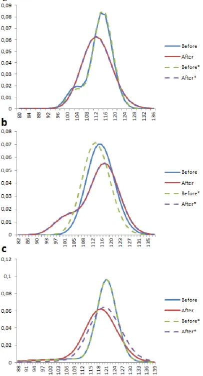
Figure 3. Comparison between pre and post curves of RND and RWD (given by “Before*” and “After*”) for (a) dotcom crisis. (b) subprime mortgage crisis. (c) European sovereign debt crisis.

Figure 3 displays the comparison between the RNDs closest to the burst of each crisis with the real world densities generated by the optimal risk aversion parameter. The six RWD shapes are given by “Before*” and “After*”. For the dotcom case, the RWD before shows a slight movement to the right compared to the RND before. It shows the existence of risk premium due to the positive risk aversion of the representative investor at the time. The curves that

26 represent the period after the burst do not show any difference, possibly due to the gamma close to zero. Regarding the subprime crisis, due to the strong negative risk aversion value on the pre burst period it is possible to perceive a negative risk premium (movement to the left) when the difference between the price of the underlying asset and the risk free asset (such as Treasury bills) is negative. The post burst period shows the same characteristics as the proportional period in the dotcom bubble. While these previous two crises present slight risk premium movements solely in the pre burst periods, the sovereign debt crisis shows a positive change on the post burst stage even though it would be expected to observe the same change in its matching period due to similar risk aversion estimates.

According to previous literature the risk aversion parameter shows considerable variation, but ranging between positive values, even for different maturities and underlying assets: Rosenberg and Engle (2002) from 2,36 to 12,5 for power utility; Bliss and Panigirtzoglou (2004) average between 2,33 and 11,14 for S&P 500 and FTSE 100 in different time horizons; Epstein and Zin (1991) reported 0,4 to 1,4; Jorion and Giovannini (1993) from 5,4 to 11,9.

Liu, et al. (2007) reseach focuses on estimating real world densities based on two parametric risk transformation methods, including the power utility fucntion. To calculate the risk aversion transformatio parameter (gamma) they use 126 consecutive expiry months, while in this research, only 10 are used for each analysed period. In Bliss and Panigirtzoglou (2004) paper, a similar number of periods was considered for the four weeks forecast horizon gamma estimation. Therefore, one possible action that could be taken to avoid obtaining negative risk aversion estimates would be to increase the amount of RNDs considered to generate the gammas. Including more periods would generate a more general risk aversion, which according to theory, should be positive. However, it is important to add that throughout the process of accumulation RNDs there was no specific pattern of improvement on the sign of the gammas from the first RND considered to the last, as it is possible to observe in table 4. Additionally, even if increasing the number of periods was a solution, there would be an evident trade-off, since having a too generalised measure would probably become useless to study any patterns created by crises or for any other purpose of comparison between periods.

27 Table 4

Evolution of accumulated gammas as more periods were considered.

Number of RNDs Dotcom Subprime Sovereign

Before After Before After Before After

-29,25 -0,92 4,75 -47,76 14,49 0,83 1 -11,50 -1,22 -4,17 -5,66 0,35 1,40 2 -11,76 -0,25 -11,11 -2,31 6,53 4,23 3 -9,40 1,34 -8,08 -2,36 0,46 5,52 4 -7,45 0,14 -6,69 -2,87 5,10 6,75 5 -5,84 -0,59 -3,81 -2,49 7,51 4,93 6 -4,29 1,13 -9,71 -1,46 9,31 2,05 7 -2,82 0,16 -7,04 -1,25 10,33 3,37 8 -2,21 -0,05 -7,62 -0,37 7,99 N/A 9 -0,27 0,42 -8,12 -0,32 5,17 4,78 10 1,44 -0,14 -6,36 -0,19 5,13 5,51 Table 4

Another potential reason for the negative gammas, besides the lack of RNDs, is the model’s high susceptibility to drops of index levels. Every time the price at expiry date was lower than at the option observation date, the gamma parameter would tend to be negative. This implies that the model based on the power utility function is capturing more than just the difference between the real world and risk neutral.

Negative gammas or negative risk aversion would mean that the representative investor is risk seeker. In other words, a risk lover investor would prefer an expected payoff lower than a certain payoff (e.g. prefer £100 with probability of 50% to guaranteed £60). It is normally assumed that investors are risk averse, mainly because if a decision maker is for some situations risk lover and for others risk averse, a competitor would take advantage of its irregular decision pattern by offering transactions that the decision maker would find appealing but would result in a net loss (Alexander, 2008). However, this should not imply that there are no periods where the average investor is risk seeker, as to individuals’ lives specific situation and stimulus may provide the necessary reasons to act in a risky way. For example: cases where investors may have nothing to lose (Alexander, 2008). This situation has been previously identified by scholars such as Jackwerth (2000); and Boudoukh, et al. (1993). They provide direct or indirect evidences that negative risk aversion can be obtained and is being overlooked due to theoretical assumptions. Jackwerth (2000) finds negative estimates of the risk aversion after the crash of 1987, providing several explanations of why other scholars (Ait-Sahalia and Lo, 2000; and Rosenberg and Engle, 1997) do not obtain similar results. Consistent mispricing in the option market after the crash is blamed as the main cause for as negative risk aversion functions. This theory of a constant difference of options implied distributions between the pre and post crash (1987) has also been presented (Jackwerth and Rubinstein, 1996) even if concerning another topic than risk aversion. Boudoukh, et al. (1993) investigate the non-negativity restriction on the ex-ante risk premium (i.e. the spread between the expected return of a portfolio of stocks and the risk free rate). They find that the ex-ante risk

28 premium is negative in some market states. These states seem to be connected to periods of high Treasury bill rates. This is an indirect proof that risk aversion can be negative: risk premium only exists to compensate market participants to invest in risky assets, as they present a preference towards certain returns (existence of risk aversion); however, if the risk premium is negative, it means that investors are focusing too much on risky assets therefore increasing the premium in the risk free assets instead (negative risk aversion).

5. Conclusion

Option prices implied densities provide insightful information about future market movements and risk preferences. While the majority of papers concerning this topic aim to test the forecast ability of the distributions produced from different estimation methods, this research focus on a more practical application: understand how investors’ risk preferences change when faced with financial shocks. The goal is to gain a better understanding whether the representative investor’s risk aversion is countercyclical or not.

The process followed to obtain the risk aversion estimates requires the extraction of options implied risk neutral densities and their respective translation into real world densities, applied to three different crises: the dotcom bubble in 2001, the subprime mortgage crisis in 2008, and more recently the European sovereign debt crisis.

In order to build the risk neutral densities, two parametric methods are implemented: mixture of lognormal densities and the generalised beta distribution of the second kind. The empirical results for the Dow Jones imply that due to an inferior quality, the GB2 method is disregarded, while the MLN produces an evolution of density curves with the expected results: higher uncertainty and future expected index levels corrected downwards.

The risk transformation procedure from RND to RWD is then accomplished by using the power utility function, previously applied by Bliss and Panigirtzoglou (2004). The resulting risk aversion estimates, do not present any evident pattern of evolution from a stable financial period to a more volatile period which characterises a financial shock. Additionally it is important to mention that for some periods, the risk aversion of the average investor reached negative values. This is a suprising result due to existent theoretical assumptions about positive risk aversion. The main possible cause for this event may be the large gap of consecutive expiration dates used in this study (10) and the ones used by Liu, et al. (2007) and Bliss and Panigirtzoglou (2004) for the risk aversion estimation (aproximately 120). However, even though the results are inconsistent with the majority of the available literature, some scholars (Jackwerth, 2000; and Boudoukh, et al., 1993) provide direct or indirect evidences that negative risk aversion can occur and that is being overlooked due to theoretical assumptions.

Overall, this study documents inconclusive results. Nevertheless, several important topics are left for future research. Interesting developments would consist of either replicating this study considering more expiration dates, having in mind that too many periods would imply an

29 extremely generalised measure that would be useless to study any patterns; apply another method from the available literature; or testing the negative estimates with more sophisticated models that are beyond the focus of this paper.