Big data analytics applied to sensor data of engeneering structures: predictive methods

(1)

University Institute of Lisbon

Department of Information Science and Technology

Big Data Analytics Applied to

Sensor Data of Engineering

Structures: Predictive Methods

Filipe Galvão Chambel Caçador

A Dissertation presented in partial fulfillment of the Requirements

for the Degree of

Master in Computer Science

Supervisor

José Eduardo de Mendonça Tomás Barateiro, PhD

LNEC

Co-Supervisor

Elsa Alexandra Cabral da Rocha Cardoso, Assistant Professor, PhD

ISCTE-IUL

(2)

(3)

Resumo

Modelos preditivos são instrumentos fundamentais para a análise da segurança de barragens. São importantes para obter conclusões acerca da segurança estru-tural destas. Os dados utilizados nos modelos preditivos, são obtidos através de sensores que se encontram embutidos nas estruturas. Apesar dos algoritmos pred-itivos serem ferramentas poderosas para a análise e previsão, outras técnicas de Machine Learning e modelos estatísticos, como as redes neuronais, têm sido desen-volvidas e utilizadas nestas áreas ao longo dos anos. Devido às diferentes formas que a monitorização destas estruturas é feita, o foco está em melhorar os métodos existentes, através de uma análise comparativa. Este trabalho tem como finali-dade o desenvolvimento de uma metodologia que compare os diferentes algoritmos preditivos, como a Multiple Linear Regression, a Ridge Regression, a Principal Component Regression e as Redes Neuronais, bem como a aplicação de diferentes técnicas de separação de dados. Esta metodologia será aplicada a um caso de estudo, com a finalidade de determinar qual ou quais as combinações de variáveis que obtêm o melhor desempenho na previsão do seu comportamento.

Palavras-chave: Análise Preditiva, Aprendizagem Automática, Data Mining, Análise de Big Data, Análise Estatística, Monitorização de Barragens.

(4)

(5)

Abstract

Predictive models are fundamental instruments for providing dam safety anal-ysis. They are important tools to retrieve conclusions about the structural safety of these dams. The data for these predictive models is gathered through sensors embedded within these structures. Even though predictive models are powerful tools for analysis and prediction, other machine learning and statistical models, like neural networks, have been developed over the years. Due to the many ways dam safety analyses is performed, the focus is to improve the existing methods by comparing them with each other. This work is focused on developing the methodol-ogy that compares different predictive models, like the Multiple Linear Regression Model, the Ridge Regression Model, the Principal Component Regression Model and Neural Networks, as well as comparing different re-sampling techniques for separating the data. This methodology is applied to a case study, with the pur-pose of finding which combinations of input variables provide the highest accuracy for predicting the behavior of these structures.

Keywords: Predictive Analytics, Machine Learning, Data Mining, Big Data, Statistical Analysis, Dam Monitoring.

(6)

(7)

Acknowledgements

The path to the completion of this dissertation proved not to be as easy as it was thought in the beginning. Its completion is thanks, in great part, to a group of special people who challenged and stuck with me through its development.

I would like to express my deepest appreciation to my Supervisor, Professor José Barateiro whose enthusiasm in this area of studies and feedback provided great insights to the development of this dissertation.

I would also like to express my gratitude to my Co-Supervisor, Professor Elsa Cardoso, whose support and thoughtful feedback provided the development of a more thorough dissertation.

A thank you to my good friend, António Antunes, with whom I shared my college experience with and throughout the development of this dissertation.

To my family a big thank you as well, for bearing with me through the difficult times, late nights and absences while writing this dissertation.

I am also greatfull for the institution LNEC for providing me with the data sources thus allowing me to have a more realistic approach on the development.

A great thank you to the institution ISCTE-IUL in which i took my bachelors and masters, by giving me the tools to further my education as well my personality.

(8)

(9)

List of Figures

1.1 Structural Health Monitoring, manual inspection and automatic

data retrieval . . . 2

1.2 Design Science Research Methodology . . . 4

1.3 Adaptation Design Science Research Methodology . . . 5

2.1 Adaptation Design Science Research Methodology - Related Work . 10 2.2 KDD Process . . . 13

2.3 CRISP-DM Methodology . . . 13

2.4 Exemplification of an outlier in a plot . . . 16

2.5 Example output of a Linear Regression . . . 19

2.6 Example of a neuron . . . 21

2.7 Example of a neural network . . . 22

2.8 Models evaluation lifecycle . . . 23

2.9 Hold-Out Re-Sampling Method . . . 26

2.10 Example of Rolling-Origin Cross-Validation . . . 27

2.11 Example of a resulting quantitative interpretation model from Gest-Barragens of a structural behavior response . . . 28

2.12 Plot of MDAS and ADAS Measurements over the years . . . 29

3.1 Adaptation Design Science Research Methodology - Design and De-velopment . . . 36

3.2 Dam Schema . . . 37

3.3 Design and Development Methodology Diagram . . . 42

3.4 Development Methodology Diagram (step one) . . . 43

3.5 Development Methodology Diagram (step two) . . . 44

3.6 Development Methodology Diagram (step three) . . . 45

4.1 Adaptation Design Science Research Methodology - Demonstration and Evaluation . . . 48

4.2 Opening variable for the cos(d) + sin(d) + h4 _{predictors combination 49} 4.3 Slippage variable for the COSD+SEND+H4 predictors combination 50 4.4 Displacement variable for the COSD+SEND+H4 predictors combi-nation . . . 51

4.5 Radial Displacement variable for the COSD+SEND+H4 predictors combination . . . 52

4.6 Tangential Displacement variable for the COSD+SEND+H4 pre-dictors combination . . . 53

(12)

List of Figures

4.7 Opening variable comparison from MLR and RR . . . 56 4.8 Slippage variable comparison from MLR and RR . . . 56 4.9 Displacement variable comparison from MLR and RR . . . 57 4.10 Radial Displacement variable comparison from MLR and RR . . . . 57 4.11 Tangential Displacement variable comparison from MLR and RR . 57 4.12 Opening variable comparison from MLR and PCR . . . 59 4.13 Slippage variable comparison from MLR and PCR . . . 59 4.14 Displacement variable comparison from MLR and PCR . . . 60 4.15 Radial Displacement variable comparison from MLR and PCR . . . 60 4.16 Tangential Displacement variable comparison from MLR and PCR . 60 4.17 Opening variable comparison from MLR and NN . . . 62 4.18 Slippage variable comparison from MLR and NN . . . 62 4.19 Displacement variable comparison from MLR and NN . . . 62 4.20 Radial Displacement variable comparison from MLR and NN . . . . 63 4.21 Tangential Displacement variable comparison from MLR and NN . 63

(13)

List of Tables

2.1 Survey on Related work about Predicting Dam Behavior Responses 30

3.1 Recording Instruments existing on the studied dam (instruments

names in portuguese) . . . 38

3.2 Provided dependent variables . . . 40

4.1 Metrics for the Opening Response . . . 49

4.2 Metrics for the Slippage Response . . . 50

4.3 Metrics for the Displacement Response . . . 52

4.4 Metrics for the Radial Displacement Response . . . 53

4.5 Metrics for the Tangential Displacement Response . . . 54

4.6 Metrics for the Response Variables for comparing MLR and RR . . 55

4.7 Metrics for the Response Variables for comparing MLR and PCR . 58 4.8 Metrics for the Response Variables for comparing MLR and NN . . 61

4.9 Metrics for the Response Variables for comparing MLR and NN using the K-Fold Cross-Validation Re-Sampling method . . . 65

(14)

(15)

Abbreviations

LNEC Laboratório Nacional de Engenharia Civil DSR Design Science Research

DSRM Design Science Research Methodology BI Business Intelligence

IoT Internet of Things DM Data Mining ML Machine Learning

KDD Knowledge Discovery Process

CRISP-DM Cross Industry Standard Process for Data Mining DM-LC Data Mining Life Cycle

SL Statistical Learning

PCA Principal Component Analysis SVD Singular Value Decomposition PC Principal Component

LR Linear Regression

MLR Multiple Linear Regression LS Least Squares

RSS Residual Sum of Squares RR Ridge Regression

PCR Principal Component Regression NN Neural Network

MLP Multi-Layer Perceptron R Correlation Coefficient R2 Coefficient of Determination

R2Adj Coefficient of Determination Adjusted MSE Mean Squared Error

RMSE Root Mean Squared Error MAE Mean Absolute Error HO Hold-Out

(16)

Abbreviations

KFCV K-Fold Cross-Validation

LOOCV Leave-One-Out Cross-Validation SWCV Sliding Window Cross-Validation SHM Structural Health Monitoring

(17)

Chapter 1 Introduction

Engineering structures like bridges, dams and buildings, have become indispens-able instruments for human society. These structures ensure and provide a diverse range of benefits, from an economic, social or environmental point of view. Once these structures are built and constantly used they start aging and begin to de-teriorate. Due to the constant usage and environmental effects suffered by these structures and the growing vulnerability associated with their aging, there has been an increasing need to assess, manage and monitor the risks associated with them, as well as to provide constant improvements to their safety throughout their entire lifespan, meaning that their structural integrity and maintainability must be guaranteed in order to prevent possible catastrophic events that may occur, either economic, environmental or humanitarian.

With these problems in mind, the goal of structural health monitoring (SHM) of engineering structures consists in determining with high accuracy the location and severity of damages on the structures as soon as they happen. The methods that are currently being used for structural health monitoring can only determine whether there is an existing damage within the structures but not the entirety extent of these damages (Chang, Flatau, & Liu, 2003).

To monitor, assess and evaluate these structures several factors must be taken into consideration to make sure that these structures are functioning as intended and to provide a way of detecting any abnormal behavior that could endanger their safety and the safety of the surrounding areas. These factors are gathered either through manually inspections by the engineering teams or specialists from these areas, or automatically by instrumentation within and around these structures,

(18)

Chapter 1. Introduction

mainly through the use of sensors, but it can also be generated based on knowl-edge from engineering experts. Figure 1.1 exemplifies these situations where the Experimenter can be identified as the visual inspector and the Embedded sensor as the automatic instrument generating the necessary information, both monitoring a structure that is interacting with its surrounding environment.

Figure 1.1: Structural Health Monitoring, manual inspection and automatic data retrieval (Balageas et al., 2010)

The most important factors that allow the monitoring of these structures are, when applied, the level and temperature of the water, air movement and temper-ature, the weight and movement of external elements on the structure, structural shifts, the age of the structure, among others. Despite the existence of instruments capable of obtaining most of these factors automatically, there is still the need for visual intervention and inspection to determine the possibility of existing unde-tected damages or deterioration. The task of getting reliable measurements from the instruments located within the structure is not easy, due to their placement often in hostile environments, where they are not easily reachable or the condi-tions inside the structure are not favorable for mechanical or electronic tools, like humidity for instance, which can, in time, cause these instruments to malfunction and provide unreliable information.

The emerging ability to acquire data from several different sources creates a new and different paradigm where science is now able to generate knowledge from pattern detection, correlations or dependencies from sources with different properties or representations. In the case of sensors, a great level of potential can be gathered from the data where they represent real events, and can easily assume a great volume of information, leading to a Big Data scenery where this generated information can aid analysts adding more value to businesses and find hidden knowledge that was not previously identified. It is very important to correctly

(19)

analyze the data to further rely on the engineering structures either when they are functional and in use or abandoned, and to be able to assess their ability to withstand unlikely events like earthquakes or other environmental causes.

Engineering structures like dams, which will be the focusing structure covered throughout the dissertation, are artificial reservoirs that are able to hold large amounts of water, ensuring a diverse range of benefits, either from an economic or from a social point of view, where their roles are to prevent floods, generate and provide hydroelectric power, to reclaim land that otherwise would be submerged and to provide water supply to several human activities, either for consumption or industrial use. Water, especially fresh water, is relatively scarce and needs to be preserved and so, it is imperative to ensure the successful monitoring of these structures. Thus, this dissertation proposes an approach for monitoring and evaluating dam response behavior based on the analyses of predictive, statistical and machine learning modeling techniques for the assessment of the structural engineering safety and maintainability of this type of structures.

The research methodology followed throughout this dissertation is the Design Science Research Methodology (DSRM) for developing and evaluating the success-fulness of the artifacts to solve the identified research problems (Von Alan, March, Park, & Ram, 2004); (Peffers, Tuunanen, Rothenberger, & Chatterjee, 2007).

1.1 Research Methodology

The Design Science Research Methodology (DSRM) focuses on the importance of creating, developing and evaluating different artifacts to meet and solve the pro-posed and relevant objectives and problems. According to (Von Alan et al., 2004), Design Science Research (DSR) is a problem-solving process which means that its main objective is the acquisition of knowledge and understandability of the prob-lems and their respective solutions to allow for the development and application of these created artifacts. And so, the authors propose seven DSR guidelines to be followed in order to prove the successfulness of each of the artifacts. The guidelines are presented as follows, including a very brief explanation about each of them:

1. Design as an Artifact: DSR must produce successful and viable artifacts that can either be defined as a construct, model, method or instantiation artifacts;

(20)

2. Problem Relevance: The objective of DSR is to develop solutions capable of solving either technological or relevant business problems;

3. Design Evaluation: The utility, quality and efficacy of each of the created artifact must be demonstrated though proper evaluation methods;

4. Research Contributions: Effective DSR must provide contributions that are able to be verified in the areas of focus of each of the artifacts;

5. Research Rigor: DSR relies on the application of rigorous methods for developing, demonstrating and evaluating the artifacts;

6. Design as a Search Process: An effective artifact requires using all avail-able means to reach a desired end under the scope of the environment of the problem;

7. Communication of Research: DSR must be presented to both, techno-logical and management oriented audiences.

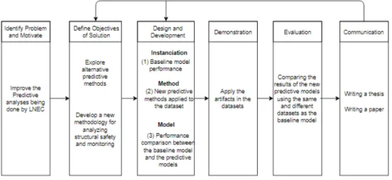
To (Peffers et al., 2007), the DSRM revolves around six main steps: (1) problem identification and motivation, (2) definition of the objectives, (3) the design and development of a proposal for the solution, (4) demonstration of the use of the developed proposal, (5) evaluation of the proposed artifacts and their results and (6) communication. Depending on the type of investigation, its entry point can vary depending on the problem at hand. In the case of this dissertation, the entry point is a Problem-Centered Initiation because in this case the objectives, as suggested in both Figure 1.2 and Figure 1.3, can only be inferred from first defining the problem and its motivation (Section 1.2).

Figure 1.2: Design Science Research Methodology (extracted from (Peffers et al., 2007))

(21)

Figure 1.3: Adaptation Design Science Research Methodology (extracted from (Peffers et al., 2007))

The artifacts that have been developed in this dissertation are: an instantia-tion artifact which focuses on analyzing the currently used (Baseline) methods; a method artifact for the identification of other predictive models for monitoring the behavioral responses of the structures; and a model artifact for the comparison of the predictive algorithms identified, against the baseline as well as against each other. The combination of these artifacts and the possibility for some improve-ments from these models are supposed to lead to advanceimprove-ments on the current body of knowledge for the identified problem.

The artifacts demonstration is done through their application on a case study with data from a real dam in Portugal which has been provided by the GestBar-ragens software developed and currently being used by Laboratório Nacional de Engenharia Civil (hereafter noted as LNEC). The focus of this demonstration is to identify the best combinations of input variables for the models and the response variables themselves, with the goal of obtaining a generic approach to the prob-lem as well as obtaining a higher accuracy in predicting the behavioral structural responses. The evaluation of the artifacts is done using a framework proposed by (Von Alan et al., 2004) and using the identified model and combination of vari-ables that provide the highest accuracy from the same source of datasets, to prove the validity of each of the artifacts.

(22)

1.2 Problem Identification and Motivation

This section of the dissertation corresponds to the Problem Identification and Motivation step of the DSRM, which purpose is to define and justify the research problem and what value will be given by applying the proposed solution.

The main problem, shared by several authors in the area, is the limited mon-itoring and representation currently being applied to the engineering structures that, in time, provide for a loss of information that could endanger the structures culminating in disaster. The application of models to predict the behavior of structural responses has become a standard for SHM. But for the most part, the input variables are chosen without considering the best combination for each of the behavioral responses. On one hand, it is expected that area specialists (i.e. civil engineers) know which variables to choose from to positively affect the response variables, thus generating high accuracy models. But on the other hand, there are other unexpected factors that could impact the structures response, such as the existence of patterns not yet discovered that could prove to be beneficial, thus increasing the predictions, and that could also provide higher insights on how the safety of these structures should be monitored and maintained.

The motivation of this dissertation derives from the necessity of improving the monitoring of the behavioral structural responses, using different predictive model techniques and input variables combinations as well as other differentiating fac-tors that could allow for beneficial improvements to the models. The success of the proposed research could provide a significant positive impact on the analysis and monitoring of generic engineering structures and their behavioral structure response. The case study used to exemplify the application of the different pre-dictive model techniques is a real dam in Portugal with automatic and manual acquisition sensors.

1.3 Contributions of the Solution

Considering the definition of the problem and the motivation behind it, as well as the related work, which is comprised by the knowledge of what has been ac-complished in the past, the objectives can then be inferred. This dissertation focuses on one main objective: explore alternative predictive and statistical meth-ods as well as machine learning algorithms for structural behavior monitoring and

(23)

safety to improve results and their interpretation by the analysts, through com-parison between them and those that are currently being used. The application of these techniques has the potential to improve the predictive capabilities of en-gineering structures and structural problem monitoring and detection, facilitating interventions on these structures. Furthermore, to determine if the objectives of the solution have been correctly defined and successfully resolved, three research questions have been created:

1. Can there be a better alternate method and combination of input variables for improving the predictive accuracy of each of the different structural be-havior responses of dams?

2. Can the representation of results be improved to provide new insights and help decision-makers improve their business decisions?

3. Can the application of the methodology developed for demonstrating the created artifacts be applied to other generic engineering structures, and not only for the application on dams?

Throughout the dissertation, several artifacts have been created, focused on resolving the previously identified problems (refer to section 1.2), that are able to improve the body of knowledge already possessed as well as use this knowledge in new ways. And so, from the following artifacts, contributions provided from this dissertation can also be inferred:

• An instantiation artifact to determine the baseline model performance from the techniques currently in place that, according to (Mata, 2011), are con-sidered to be good practices for structural behavior prediction and safety on dams. This baseline model performance will then be compared to the other predictive models to determine what models, combination of input variables and necessary parameters, provide a higher accuracy of the results, considering what is currently being done.

• A method artifact for applying other predictive statistical models or ma-chine learning algorithms to the datasets and generate new models to im-prove the basis knowledge and to allow for further comparison of their per-formance against the baseline model.

• A model artifact for comparing the performance of the resulting predictive models with the performance of the baseline model performance.

(24)

The demonstration of how the developed artifacts are going to solve the iden-tified problems is done through the development of a methodology (Chapter 3) applied to a real case study (Chapter 3.1) in which, example datasets, each refer-ring to one of the five behavioral response variables considered, are going to be used for determining the performance results of each of the models that are then compared to the performance of the baseline model.

And finally, to evaluate and validate the success as well as the performance of the artifacts, taking into account the identified problems, the model artifact is then applied to different datasets to demonstrate the generalization of the artifact as well as to determine its efficiency and effectiveness.

1.4 Document Structure

The remainder of this dissertation is structured as follows:

• Chapter 2 - Related Work: In this chapter, it is provided an overview of the existent literature in the area of this research, as well as the related work on predicting the behavior of engineering structures, with a focus on Dams, as introduced in Chapter 1;

• Chapter 3 - Design and Development: In this chapter, the objectives of the solution are identified through the development of the artifacts applied on the Demonstration phase (Chapter 4) as well as the case study (Section 3.1);

• Chapter 4 - Demonstration and Evaluation: In this chapter, the pro-posed solution is applied to the datasets and the results are demonstrated and evaluated in order to determine their efficiency and validity on this re-search;

• Chapter 5 - Conclusions: In this chapter, it is concluded the dissertation, the research questions proposed on Chapter 1 are answered and is defined the future work to this research.

(25)

Chapter 2 Related Work

This chapter of the dissertation covers the theoretical background and work related to the problem and motivation that have been previously identified (Section 1.2), which allows for the definition of the objectives of the solution of the DSRM. The knowledge of the body of work contained throughout this chapter will serve as input for the advancement of the following steps of the research, as expressed in Figure 2.1.

• Section 2.1: In this section it is introduced the Big Data Analytics paradigm to motivate the capabilities of Big Data and the value that it gives to busi-nesses;

• Section 2.2: In this section it is introduced the notion of Data Mining, in order to introduce the accepted methodologies for creating a valuable Data Mining Project and the different data preparation techniques that go along with it;

• Section 2.3: In this section it is introduced the concept of Predictive Mod-eling in which are presented the different predictive models used throughout the Demonstration and Evaluation phase;

• Section 2.4: In this section there will be presented the concept of Mod-els Evaluation where are explained the different evaluation metrics and re-sampling methods used to evaluate the different predictive models;

• Section 2.5: In this section it is presented the current Predictive Model-ing techniques for Dam Behavior where the existModel-ing work, related to dam behavior monitoring, is shown.

(26)

Chapter 2. Related Work

Figure 2.1: Adaptation Design Science Research Methodology - Related Work (extracted from (Peffers et al., 2007))

2.1 Big Data Analytics

Data has been growing at an exponential rate, due to constant technological ad-vances, which in time, created the need to improve the ability to store, access, manipulate and manage data, giving the possibility for the emergence of Busi-ness Intelligence systems. BusiBusi-ness Intelligence (BI) was first introduced in 1958 by an IBM researcher (Luhn, 1958) and has been around for decades where its definition has been reviewed and improved multiple times, focusing on changing how organizations should implement their strategies and improve their decisions. The purpose of BI is to provide insightful knowledge and find useful information to provide with the decision makers the means of detailed and summarized data through use reporting tools and dashboards (Elena et al., 2011). The reporting and analyzing requirements associated with these systems tend to maintain a sim-ilar growth rate as technology itself to allow for the most valuable and on time information as possible (Nedelcu et al., 2013). (Larson, 2012) and (Kimball & Ross, 2011) agree that BI is comprised of three fundamental stages:

• Data gathering and manipulation, retrieved from different sources and incor-porated into one big repository, usually incorincor-porated into a Data Warehouse system;

(27)

• Data analyses by use of several Data Mining techniques, Machine Learning algorithms and/or Statistical models;

• Data representation techniques, like dashboards, through access and manip-ulation of the data as tools for decision makers in their decision making processes.

The rising amounts of data being generated through a diverse range of indus-tries lead to a new and interesting paradigm, which is for the moment, identified as Internet of Things (IoT), which main purpose is to enhance the potential of the data. According to (Atzori, Iera, & Morabito, 2010) data can be generated in three ways: from the Internet, from sensors or from extracted knowledge. This new data potential, quality and growing quantity allows businesses to improve their systems and by extension, their decisions, in order to gain competitive advantage over others. These amounts of data provides businesses with the realization of the importance of Big Data Analytics to support their strategies (Ularu, Puican, Apostu, Velicanu, et al., 2012); (Huisman, 2015).

Big Data Analytics adds new challenges and opportunities to BI with a sim-ilar definition, being the main difference the fact that it is used to find and re-trieve value from Big Data instead of the "normal" data businesses are used to. (Gandomi & Haider, 2015) points out that Big Data is worthless unless when used to drive the process of decision making. This assertion tells us that businesses should be more focused in applying Big Data Analytics on their data to improve their decision-making process. But on the other hand it is also true that most com-panies have huge amounts of data but these amounts can not yet be considered as Big Data.

(Assunção, Calheiros, Bianchi, Netto, & Buyya, 2015) describes BD as being a “multi-V model” where each “V” characterizes its main aspects:

• Variety, refers to the different types of data being generated and can now be used. Throughout the years the generated data has been focused on structured data that its currently being used in traditional databases, but now, the biggest part of the data that is being generated is unstructured.

• Volume, which refers to the vast amounts of data that is being generated every second;

• Velocity, which refers to the speed rate that new data is being generated and moving around;

(28)

• Veracity, which refers to the quality and control of the volume of data being generated

• Value, which refers to the value that the study of this unstructured data, provides to the growth of businesses and their decision-making processes.

To retrieve knowledge from BD, (Sun, Zou, & Strang, 2015) and (Huisman, 2015) agree that BDA is comprised of three main components: Descriptive Ana-lytics, which is often described as a summarization of historic data into knowledge and meaningful information through the discovery of existing relationships within the BD (Huisman, 2015); (Sun et al., 2015). It focuses on answering questions like “What and when did it happen?”; Predictive Analytics that according to (Buytendijk & Trepanier, 2010) is the use of several statistical, forecasting and data mining techniques to predict future events based on the descriptive data and focuses on questions like “What will happen?”; and finally, Prescriptive Analytics which tries to explain why something has happened.

2.2 Data Mining

Machines have become powerful instruments for providing the industries with the ability to automate processes that would be too time consuming if being done manually, even though, it is common that machines are sometimes unable to do simple tasks that humans are able to do with great ease. The Data Mining (DM) concept became relevant due to the growing availability of data, from IoT devices for instance, and the need to generate knowledge and information from these data. (Jain & Srivastava, 2013) and (Padhy, Mishra, Panigrahi, et al., 2012) define DM as a way of mining knowledge and improve decisions through processes of Machine Learning (ML) by exploring and analyzing large amounts of data or BD. The authors describe DM as a Knowledge Discovery Process (KDD) or as a way of extracting hidden information to predict trends and behaviors to gain competitive advantage. In contrast, (Fayyad, Piatetsky-Shapiro, & Smyth, 1996) refers to the KDD process as being composed of several tasks to extract knowledge where one of those tasks is DM where he considers it as the process of retrieving important and relevant information, like patterns, anomalies or any alterations made to the dataset. According to (Lei-da Chen, Frolick, et al., 2000) DM is used depending on the needs of the organization thus generating different types of information to find meaningful relationships between the data and to predict trends and patterns.

(29)

Figure 2.2: KDD Process (extracted from (Fayyad et al., 1996))

DM projects according to (Marbán, Mariscal, & Segovia, 2009) follow the CRISP-DM (Cross Industry Standard Process for Data Mining) methodology. This methodology, also described as the Data Mining Life Cycle (DM-LC), demon-strated in Figure 2.3, has a comprehensibly flexible sequence of phases due to the possibility to go back to each of the previous steps to improve and modify the reasoning or the variables being used.

Figure 2.3: CRISP-DM Methodology

The Business Understanding phase or Problem Identification phase is crucial when developing DM projects, because it identifies the objectives and requirements of the business and in almost every case they are the success criteria for a good DM project. Data Understanding phase includes the initial insight to the data to describe and explore it to form ideas and to find ways of retrieving hidden information. According to (Zhang, Zhang, & Yang, 2003) the Data Preparation phase takes approximately 80% of the total project and covers the steps of creating

(30)

quality data to construct the dataset that will be used as input for the modeling phase, including data selection and data cleaning. The Modeling phase is where the different modeling techniques are selected and the model is built. The Evaluation phase is where the results produced by the models will be evaluated to see if they can achieve the business requirements and objectives that were previously identified and where the knowledge is created. The Deployment phase is the end phase of the project where the knowledge gained from the Evaluation phase is deployed.

According to (Lei-da Chen et al., 2000) DM methods are divided into two main learning groups, Statistical Learning (SL) and ML. SL is defined as a tool to build statistical models to predict outcomes by having an underlying prob-ability model and combining different fields of computer science like Statistics, Artificial Intelligence (AI) and DM (James, Witten, Hastie, & Tibshirani, 2013). ML, according to (Mohri, Rostamizadeh, & Talwalkar, 2012), is defined as the use of efficiently designed computational methods or algorithms that are improved using experience or training, improving their performance and provide more ac-curate predictions.(Deshpande & Thakare, 2010) on the other hand, refers that DM should be separated into two categories, Descriptive Models and Predictive Models. This definition differs from what (Lei-da Chen et al., 2000) described in the sense that SL and ML include both Descriptive and Predictive modeling. Pre-dictive modeling problems consist in obtaining knowledge from analysis on past experiences while Descriptive modeling problems consist in analyzing the evolution of a given dataset to increase its knowledge.

2.2.1 Data Preparation and Cleaning

Data Preparation is a very important part of any Data Mining project and one of the most time consuming, including several tasks. The main goal is to generate quality data from existing raw data. When generated automatically, this data is usually “dirty” or in other words, inconsistent, noisy or with missing values.

In the Data Preparation process, if applied, there is also the need for dimen-sionality reduction. By reducing irrelevant or redundant features or even instances of the data, the efficiency, speed and accuracy of the next DM processes can be significantly improved.

(31)

By cleaning the data and selecting the features that will be used it is also possi-ble, by combining other, different features, to find and add hidden and undetected features (Zhang et al., 2003).

2.2.1.1 Incorrect and Missing Values

Most of the predictive models make the assumption that all the input data values are present and correct, hence the need to previously identify and revise incorrect and missing values. If incorrect values reach the algorithms, as to overcome them, they are either rendered insignificant or overrated which in both cases, causes a negative impact on the model response. If incorrect values cannot be interpreted by the algorithm then they are treated as a missing values and if they do not appear that frequently on the dataset than they may be considered as irrelevant (Abbott, 2014).

Missing values cause a negative impact on the accuracy of the models and are hard to deal with and so, (Grzymala-Busse & Hu, 2001) and (Abbott, 2014), consider several approaches to mitigate them:

• Replace the missing value with a new value: By using this approach, the missing values can take on the value of either the most common attribute value, a special value (-1, for instance) or the form of a mathematical arith-metic function like the average or median of the attributes values;

• Delete missing values: The simplest approach is to delete the instances con-taining the missing values, either by removing an entire row or an entire column depending on what the modeler decides. The fact that an entire col-umn or row is deleted, especially with a colcol-umn, a great deal of information is also being removed and not only the missing value, which can even cause a greater impact over leaving the missing values on the data.

2.2.1.2 Outliers

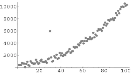
Outliers are defined as unusual values that do not present the same behavior as other values do. They are caused either by an anomaly caused by an equipment, like sensors for instance, or either by a real abnormal event, like an earthquake (Chen, Wang, & van Zuylen, 2010). The difficulty lies in dealing with outliers on the premise that not all outliers can be considered insignificant and can be

(32)

positively influence the outcome in terms of adding valuable information to the dataset. (Abbott, 2014) describes several approaches to deal with outliers:

• Removing the outlier from the dataset: This approach can reveal to be either good or bad, depending on the significance of the outlier. If the presence of the outlier proves significant then information is being lost, and if not then the model is improved;

• Transforming the outliers: Based on the same premise of the previous ap-proach of removing the outlier from the dataset, changing the nature of an outlier can also compromise the model and its response;

• Keep the outliers: This approach limits the modelers choice in which models to use, being only able to use models that are not greatly affected by the presence of outliers, or penalize their existence.

Figure 2.4: Exemplification of an outlier in a plot

2.2.1.3 Feature Selection and Dimensionality Reduction

Reducing the dimensionality of the data allows for an model to operate faster and more effectively by removing irrelevant or redundant information. This reduction can be done through feature selection providing a better understanding and inter-pretation of the data or either by the application of Principle Component Analysis (PCA) (S. Kotsiantis, Kanellopoulos, & Pintelas, 2006). Another way of gaining valuable information from the data is through adding new features or as (Abbott, 2014) defines them as “derived variables”. The commonality between reducing and

(33)

creating features is that when features are proven to be good they reduce the necessity for a more complex understanding of the data and they produce more valuable and trustworthy results.

2.2.1.4 Principal Component Analysis

According to (Abdi & Williams, 2010) and (James et al., 2013) Principal Com-ponent Analysis (PCA) focuses on the following objectives: extracting the most important information from the dataset; and reducing the dataset with the intent of only maintaining the most important information, thus simplifying its under-standability. To do this, PCA applies linear combinations to the original set of variables revealing the principal components which try to explain and reduce the existent variability of the original dataset. Before the PCA analysis can be done, all the variables must be standardized or normalized to eliminate any influences or weight that one variable might have over the rest of the variables. According to (Friedman, Hastie, & Tibshirani, 2001) PCA is computed using Singular Value Decomposition (SVD) which decomposes a matrix X (M ∗ N ) into three other matrices:

X = U ∗ S ∗ Vt (2.1) where U is a (M ∗ M ) matrix, S is a diagonal (M ∗ N ) matrix and Vt is the transpose of V , where V is a (N ∗ N ) matrix. PCA is commonly used for increasing the efficiency of the analysis of the models by reducing the redundancy of the model. It does this by reducing the dimensionality with losing the minimum amount of information. And so, the original variables that presented some form of correlation between them, are transformed into uncorrelated variables or Principal Components (PC), which are linear combinations of the correlated variables.

2.3 Predictive Modeling

Based on (Abbott, 2014), predictive modeling algorithms are supervised learning algorithms which implies that they learn based on previous experiences, in other words, they generate a new predictive response by testing a new set of input data to a known set of inputs that are already known to produce a certain response.

(34)

(Friedman et al., 2001) refers to this as a process of “learning by example”. Su-pervised Learning is usually divided into two main categories: Regression and Classification. In the Regression setting, response variables are usually charac-terized as quantitative or numerical and the main objective is to predict based on continuous measurements. In contrast, in the Classification setting, response variables are usually qualitative or categorical and the main objective is to assign a label to the response variables. The main goal of these models is to predict a given variable Y εR in terms of a set of inputs XεRv:

Y = F (X) + ε (2.2)

where F (X) is the observed value of the function in use, ε is an error term and v is the number of inputs. There are several predictive algorithms (regres-sion, neural networks, decision trees, k-nearest neighbors, etc.) but throughout this dissertation the focus will be mainly on neural networks and on regression algorithms, such as: Multiple Linear Regression, Ridge Regression and Principal Component Regression, as they provide a far better comprehension of quantitative results.

2.3.1 Multiple Linear Regression

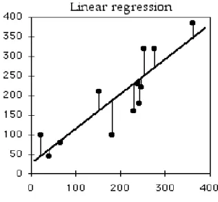
Linear Regression is the most basic and commonly used predictive model where its purpose is to explain the existing relationship (the weight or value of the coeffi-cients) between a dependent variable Y or response, and one or more independent variables X or predictors (James et al., 2013). In other words, Linear regression provides a general description of how the inputs affect the output by weighing the coefficients (Friedman et al., 2001). Depending on the number of independent variables when applying Linear Regression, it can either be described as Simple Linear Regression when only one independent variable is used or Multiple Linear Regression (MLR) otherwise. The Multiple Linear Regression model is represented by the following equation:

F (X) = β0+ P

X

j=1

∗Xj ∗ βj (2.3)

Where β0...P corresponds to the coefficients, X1...j to the independent variables

(35)

al., 2001), the independent variables can be considered by taking on several forms, mainly as quantitative inputs, as transformations of those quantitative inputs, like the logarithm for example, of the polynomial representation of those inputs (X2_,

X3, X4) or of arithmetic interactions between the variables, like X3 = X1∗ X2 for

instance.

Figure 2.5: Example output of a Linear Regression

(Friedman et al., 2001) also refers that in most of the cases where the appli-cation of Linear Regression is prominent, the coefficients are usually calculated through the Least Squares, in which the coefficients are chosen to minimize the Residual Sum of Squares (RSS), given by Equation 4 and to find the best fit to the data. RSS(β) = N X i=1 (yi− F (X)))2 (2.4)

Sometimes the Least Squares method does not provide the best accuracy or interpretation of the model due to the possibility that some predictors can present a large variance of their data which means that they provide little to almost no additional information to the model, and if large number of predictors are used, then the interpretation of the model becomes a lot more complex (Friedman et al., 2001).

The interpretability of Linear Regression models can be done in two different ways: (1) through the values of the coefficients that describe the weight that

(36)

is given to a certain predictor variable and how they will impact the estimated values; (2) by comparing the values of the response variable or estimated values, with the actual values of the model by use of error measures as will be discussed afterwards in Section 2.4 (Abbott, 2014). (Tobias et al., 1995) refers that to take full advantage of the MLR models, three different conditions should be met: (1) the predictors that are used to express a response must be few; (2) there must not be any correlation between them (which as explained in 2.2.1.4 could be achieved through the use of PCA) or in other words, there must not have a highly linear relation, and (3) they must express some sort of relationship to the responses.

2.3.2 Ridge Regression

According to (Friedman et al., 2001), the idea of Ridge Regression (RR), also de-scribed as the Tikhonov regularization, is to penalize the regression coefficients. This algorithm is similar to the MLR algorithm, where the only noticeable differ-ence is in the application of a lambda (λ) parameter that controls the amount of penalty going that is going to be applied to the coefficients, thus allowing for a more controlled shrinkage of the model by shrinking the coefficients towards zero, which causes a smoothing the model. This method provides a decorrelation of the variables, without applying any sort of dimensionality reduction like PCA. Just like MLR, RR uses the Least Squares method to minimize the RSS but in this case, it considers the influence of the penalty on the coefficient to minimize the sum of the squares, as shown in Equation 2.5. If the value of the coefficients (β) is large than the value for the penalty will increase.

RSS(λ) = (y − Xβ)T ∗ (y − Xβ) + λβT_β _(2.5)

Where λ is the amount of shrinkage to be applied to the model and X is the input matrix.

2.3.3 Principal Component Regression

Sometimes, there are a large number of independent variables that can sometimes be correlated between them and so Principal Component Regression (PCR) is a linear predictive model which estimates the response of the model based on the selection of Principal Components (PC) that represent the most explanatory

(37)

variables by making use of PCA that has been discussed in 2.2.1.4 Since the PCs don not present any sort of correlation between them, they are then considered as inputs for the model (Liu, Kuang, Gong, & Hou, 2003). According to (Friedman et al., 2001), the PCR starts by standardizing the inputs, and only then is the PCA algorithm applied so that there are only PC applied to the regression instead of the original predictors. By standardizing and applying the PCA to the model, reducing the dimensionality of the model, PCR takes care of any possible collinearity or correlation between the predictors. By considering Equations 2.1 and 2.5 (refer to 2.2.1.4 and 2.3.2, respectively), the representation of the PCR model becomes:

X = z1v1T + z2v2T + ... + ziviT + ε (2.6)

where z1...i are the score values, v1...i are the eigenvalues of the matrix X and

ε is the error term.

2.3.4 Neural Networks

Neural Networks are defined as Multi-Layer Perceptrons (MLP). MLPs are com-prised of neurons, where each neuron is defined by an equation, usually referred to as a transfer function (Abbott, 2014).

Figure 2.6: Example of a neuron (extracted from (Abbott, 2014))

A single neuron can produce a linear model. Using a single neuron does not provide better results than by using other predictive models because there are several linear models that have greater accuracy and are more efficient. To show improvements when compared to linear models, neural networks stack these single neurons in layers allowing for more powerful and flexible prediction algorithms.

(38)

As said, a layer is a set of stacked neurons, and can be defined either as an input layer, output layer or hidden layer. The hidden layers are usually between the input and the output layer.

Figure 2.7: Example of a neural network (extracted from (Abbott, 2014))

Neural Networks are iterative learners which means that they learn step by step. In the first step the weights are randomly initialized in order to start training the algorithm, passing through the different layers of the network ending up on the hidden layers and finally in the output layer. The resulting prediction is compared by measuring the error, to the actual expected value. The weights are then adjusted with the calculated error measured and a new cycle or epoch starts. This happens until the entire dataset is trained, thus being ready to be tested with new unknown values.

2.4 Models Evaluation

Predictive models are developed based on past data, that will then be applied to new instances of data that have not yet been introduced in the models, or in other words, new generated data. It is necessary to evaluate and verify these in terms of accuracy and performance when confronted with new data.

The evaluation of the performance of the models is usually divided using dif-ferent or a combination of several re-sampling methods into two sets, the training set and the test set (Figure 2.8). Sometimes a third set may also be considered where it is defined as the validation set. And so, this evaluation is made through the use of an evaluation measure (or error measure) in mind. To estimate the

(39)

accuracy and performance of this models is to provide a method for comparing the models between them to be able to fine tune these models.

Figure 2.8: Models evaluation lifecycle

2.4.1 Criteria for Model Comparison

Many criteria, that can also be defined as accuracy measures, are used to estimate how well the models are performing, their purpose is to measure the difference between the estimated or predicted values and the actual or real values:

ei = yi− ˆyi (2.7)

Where yi is the real value and ˆyi is the estimated value of the model. Accuracy

measures are scale dependent which means that they cannot compare values with different scales. This information is then used by the modelers, so that they can fine tune these models in order to either improve them or decide that it is not worthy using them in the long run (James et al., 2013).

2.4.1.1 Correlation Coefficient

Correlation Coefficient or R measures the linear relationships between the ables. It focuses on quantifying the dependence or correlation between the vari-ables. It ranges from [-1.0,1.0] where it indicates either a negative or positive correlation between the variables, respectively. If the result equals to 1.0 then there is a perfect positive linear correlation between x and y, presenting the same amount of variation. If, by contrast the result equals to -1.0, then there is a perfect negative linear correlation between the variables which means that they vary in an opposite way. If the result equals to 0 then there is no correlation between them.

(40)

The most common calculation for the Correlation Coefficient is through the Pearson product-moment, where its first calculated the covariance between the variables and then is divided by their standard deviations:

Rxy =

Cov(vx, vy)

σx∗ σy

(2.8)

Where v(x, y) corresponds to the real and estimated variables and σ(x, y) cor-responds to each of the variables standard deviations.

2.4.1.2 Coefficient of Determination

Coefficient of Determination or R2_{, measures how well the model can predict}

future outcomes, in other words, how well the dependent variables can be predicted considering the independent variables. It accounts for the variability of the model and it is calculated through the square of the Coefficient Correlation and it ranges from [0.0,1.0]:

R2_xy = (Cov(vx, vy) σx∗ σy

)2 (2.9)

An improvement can be made to the R2_{, that is defined as the Coefficient of}

Determination Adjusted or R2

adj, which gives the percentage of variation that the

independent variables are really affecting the dependent variable, in other words, with provides the confidence of the model predicting the correct outcome.

2.4.1.3 Mean Squared Error

Mean Squared Error or M SE measures the quality of the estimated value or, in other words, how close the estimated values differ from the actual values. The M SE of the predictions is the mean of the squares of difference between the estimated value and actual values and it can be defined as:

M SE = 1 n n X i=1 (ei)2 (2.10)

Where n is the number of instances within the dataset and ei is the error

(41)

that are close to 0 are highly desirable, because if the estimate for the predictive value is 0, then the algorithms accuracy was perfect. The M SE is extremely useful because it shows the variance and deviation from the estimated value to the actual value (James et al., 2013).

A variation of the M SE can be defined as the Root Mean Squared Error or RM SE, where nothing more than the root of the M SE metric. This is an useful metric due to its ability to amplify through penalization, large errors that by using only the M SE would most likely pass undetected.

RM SE = v u u t 1 n n X i=1 (ei)2 (2.11)

2.4.1.4 Mean Absolute Error

The Mean Absolute Error or M AE is the sum of the absolute values of the errors. The advantage of applying this metric rather than M SE is when dealing with outliers. Despite the outliers, M AE accuracy follows the same logic as M SE being that it is better when closest to zero. M AE is defined as:

M AE = 1 n n X i=1 |ei| (2.12)

2.4.2 Re-sampling Methods

Re-sampling methods are used to determine and/or increase the accuracy of a model by refitting a model to retrieve new hidden information that sometimes can only be obtained by fitting the model more than one time. This process of evaluating the performance of a model is also defined as model assessment (James et al., 2013). According to (S. B. Kotsiantis, Zaharakis, & Pintelas, 2007) there are two ways for evaluating the predictive accuracy of a model: (1) by splitting the dataset into training and testing sets or Hold-Out and (2) through K-Fold Cross-Validation. (James et al., 2013) refers an additional variance of cross-validation referred to as Leave-One-Out Cross-Validation.

According to (Tashman, 2000) in order to provide a real-time assessment for forecasting, there is a need to wait a long time for data to be generated in order

(42)

to get a reliable picture of what is going to be forecast. He also refers that the Hold-Out method has become the most generally accepted re-sampling method.

2.4.2.1 Hold-Out

Hold-Out is one of the simplest and easiest validation techniques by randomly splitting the training and the tests sets only once (usually dividing 2₃ of the data to the training set and the other 1₃ to the test set) as exemplified in Figure 2.9 (James et al., 2013). For predictive models that, to provide better results, account for most of the historical data, usually the training set takes up 80 to 95% of the records on the dataset.

Figure 2.9: Hold-Out Re-Sampling Method

2.4.2.2 K-Fold Cross-Validation

K-Fold Cross-Validation (K-Fold CV) takes the same approach as Hold-Out but instead of splitting the dataset only once it splits it k times, usually of the same size. The k=0 subset is used as the validation set and the remaining k-1 subsets are treated as the training set. The model repeats k times where each time the validation set changes. One variation of the K-Fold Cross-Validation is the Leave-One-Out Cross-Validation (LOOCV) which follows the same logic as the K-Fold CV where the k times that the model is split corresponds to the number of elements with the dataset. In other words, the dataset is trained and tested k (number of elements minus one) times (James et al., 2013).

2.4.2.3 Rolling-Origin Cross-Validation

Rolling-Origin Cross-Validation or ROCV is an out-of-sample evaluation, in which the the origin of the training set is successively being updated, much like the Slid-ing Window method, which results in the production of several new forecasts

(43)

(Tashman, 2000). Assuming the division of a dataset with 10 years into N=10, where N is the number of samples, each corresponding to a year of records. The ROCV maximum number of samples would be N=5, where the last sample cor-responds to the test set and the other 4 to the training set. The forecast is then generated and the ROCV moves forward one until it reaches the tenth sample, thus generating 5 forecasts.

Figure 2.10: Example of Rolling-Origin Cross-Validation

2.5 Predictive Modeling for Dam Behavior

Structural Health Monitoring (SHM) has been growing and evolving over the years, mainly with the appearance and evolution of sensor technologies to identify struc-tural damages. It offers automated methods for assessing the strucstruc-tural integrity and health through structural monitoring systems. These systems have been con-tinuously growing and being improved, and are widely accepted for the detection and prediction of the behavior of the structures and are responsible for collect-ing the measurements from the sensors that are installed within these structures (Lynch & Loh, 2006).

GestBarragens is a software for monitoring the safety of engineering structures like dams, which supports, among others not relevant for the scope of this research, the process of manual and automatic data exploration from instruments located on the structures, the process of visual inspections as well as the ability for anomaly

(44)

detection, to ensure a good decision-making process (Silva, Galhardas, Barateiro, & Portela, 2005).

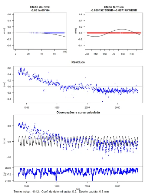
GestBarragens also supports the generation and visualization of quantitative interpretation models, numerical models as well as physical models. The quan-titative interpretation models establish relations between the input values that influence the model and the structural behavior responses, as exemplified in Fig-ure 2.11 (Portela, Pina dos Santos, Silva, Galhardas, & Barateiro, 2005).

Figure 2.11: Example of a resulting quantitative interpretation model from GestBarragens of a structural behavior response

Other challenges like the one proposed by (Mata & Tavares de Castro, 2015) also have the intention of providing better and quality data to allow for a better further analysis. The authors propose a qualitative analyses and assessment of

(45)

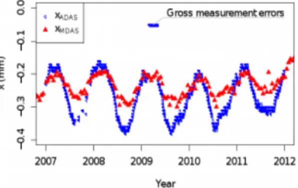
paired samples of automatically and manually gathered measurements (ADAS and MDAS, respectively). Their idea is to eliminate gross measurements resulting from the difference in frequency of gathered records, pairing both the ADAS and the MDAS to determine through the use of Probability Density Functions (pdf) if they represent the same population, thus eliminating differences between the ADAS and MDAS, to successfully analyze the ADAS measurements (Figure 2.12).

Figure 2.12: Plot of MDAS and ADAS Measurements over the years

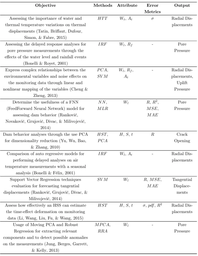
There has been a significant amount of work done relative to monitoring the behavior and safety of dams. For a more general perception of what has been done in this area, several related papers have been analyzed and summarized in Table 2.1. These papers have been characterized in several dimensions: (a) the objective of the paper, (b) the models used, (c) the input attributes for the models (environmental variables), (d) the error metrics for model validation and (e) the output of the model (dam behavior).

(46)

Table 2.1: Survey on Related work about Predicting Dam Behavior Responses

Objective Methods Attribute Error

Metrics

Output

Assessing the importance of water and thermal temperature variations on thermal

displacements (Tatin, Briffaut, Dufour, Simon, & Fabre, 2015)

HT T Wt, At σ Radial

Dis-placements

Assessing the delayed response analyses for pore pressure measurements through the effects of the water level and rainfall events

(Bonelli & Royet, 2001)

IRF Wl, Rf - Pore

Pressure

Express complex relationships between the environmental variables and noise effects on

the monitoring data through linear and nonlinear mapping of the variables (Cheng &

Zheng, 2013) P CA, SV M Wl, Rf, At - Radial Dis-placements, Uplift Pressure

Determine the usefulness of a FNN (FeedForward Neural Network) model for

assessing dam behavior (Ranković, Novaković, Grujović, Divac, & Milivojević,

2014) N N , M LR Wl R, R2, M SE, M AE Pore Pressure

Dam behavior analyses through the use PCA for dimensionality reduction (Yu, Wu, Bao,

& Zhang, 2010)

HST , P CA

H, S, t R Crack

Opening

Comparison of auto regressive models for performing delayed analyses on air temperature measurements with a seasonal

analysis (Bonelli & Félix, 2001)

IRF Wl, At - Radial

Dis-placements

Support Vector Regression techniques evaluation for forecasting tangential displacements (Ranković, Grujović, Divac, &

Milivojević, 2014) SV M Wl R, M SE, M AE Tangential Displace-ments

Assess how effectively an HSS can estimate the time-effect deformation on monitoring

data (Li, Wang, Liu, Fu, & Wang, 2015)

HST H, S, t σ, pdf , R2 _Radial

Dis-placements

Usage of Moving PCA and Robust Regression for extracting relevant components and to detect possible anomalies on the measurements (Jung, Berges, Garrett,

& Kelly, 2013)

M P CA, RRA

Wl - Pore

(47)

Application of a statistical approach accompanied with a structural identification

technique to provide a higher degree of accuracy in predicting and monitoring the

behavior of dams (De Sortis & Paoliani, 2007)

HST H, S, t R, σ Radial

Dis-placements

Application of a Feed Forward Neural Network to estimate and simulate the flow of

a dam (Tayfur, Swiatek, Wita, & Singh, 2005)

N N Wl RM SE,

M AE, R2

Pore Pressure

Performance comparison between a MLR and a NN model for assessing dam behavior

(Mata, 2011) M LR, N N Wt, At M AE, M axAE, R Horizontal Displace-ments Increase fitting accuracy and forecasting

precision based on an Error Correction Model by integrating the relationships between the output and input variables (Li,

Wang, & Liu, 2013)

ECM , M LR H, S, t, error σ, pdf , R2 _Radial Dis-placements

Identification of the effect of air temperatures on the structural response of the dam based

on a Fourier Transform analysis (Mata, de Castro, & da Costa, 2013)

ST F T H, At σ, R2 Horizontal

Displace-ments

Usage of modifications of the PLS model for mitigating the collinearity between the variables and the existence of outliers, and

the selection of informative variables (Xu, Yue, & Deng, 2012)

SIM P LS, GA −

P LS

H, At RM SE Crack

Opening

Assessing the performance of a MLR model optimized by using Genetic Algorithms

(Stojanovic, Milivojevic, Ivanovic, Milivojevic, & Divac, 2013)

M LR H, At,

Ct, Rf, t

R2_{, RM SE} _Radial

Dis-placements

Assess the performance of hybrid models for dam deformations (Perner & Obernhuber,

2010)

M LR H, Ct, t - Radial

Dis-placements

Methods: HT T =Hydrostatic Thermal Time; IRF =Impulse Response Function; P CA=Principal Component Analysis; SV M =Support Vector Machines; N N =Neural Networks; M LR=Multiple Linear Regression; HST =Hydrostatic Seasonal Time; M P CA=Moving PCA; ECM =Error Correction Method; ST F T =Short Time Fourier Transform; SIM P LS=Statistically Inspired Modification of Partial Least Squares;

GA − P LS=Hybrid Genetic Algorithm with SIMPLS.

Attributes: Wt: Water Temperature; At: Air Temperature; Wl: Water Level; Rf:

Rainfall; H: Hydrostatic; S: Season; t: time; C_t: Concrete Temperature.

Error Metrics: σ: Standard Error of Estimate; R: Correlation Coefficient; R2: Coeffi-cient of Determination; M SE: Mean Squared Error; RM SE: Root Mean Squared Error; M AE: Mean Absolute Error; pdf : Probability Density Function; M axAE: Maximum

(48)

The main contributions provided by these authors are the identification of different models used to monitor structural damages in dams through the rela-tionships between the environmental variables (predictors) and the behavior of the dams (response). Depending on the problem and the case study, several objectives have been defined but the commonality between them is the analyses of the moni-toring data either being generated manually or by equipment within the structures (pendulums, piezometers, etc.), and the identification of responses that explain the behavior of these structures (pressures, displacements, etc.). Even though most of the authors provide different alternative models for monitoring dam behavior, most of the attributes or environmental variables that serve as inputs for these models are the same: Hydrostatic Load, Water Level, Air Temperature, Water Temperature, Rainfall, Time.

2.5.1 Dam Behavior variables

According to (Mata, 2011) and (Xu et al., 2012), and considering the attributes of Table 2.1, the statistical relationship between the dependent variables and the independent variables is given by:

Y (W, T, t) = YW + YT + Yt+ ε (2.13)

where the Y (W, T, t) corresponds to the response variable, the W corresponds to the Hydrostatic Load, the T to the Temperature variations, the t to the time since the initial record of the structure, or in other words, the aging of the structure and ε to the error component. Each of the effects of components that correspond to each of the independent variables provide different influences on the behavior of the structure.

The influence of the YW variable can be described through the use of

polyno-mials to scale this variable in order to provide more weight to these variable and thus giving it more influence if necessary to the models, where β1...4 correspond to

the coefficients to adjust and the h = 265 − 76, where 265 is the Crest Elevation and 76 is the Height Above Streambed, which corresponds to the water level:

(49)

According to (Mata, 2011) the influence of the temperature can be calculated through the use of the age of the structure, and can be considered as a sinusoidal function, extending over a period of a year or six months (In the context of this dissertation, the functions have been calculated for a period of a year). This function can be extracted in this form, especially in the case of Portugal, since the country has a sort of predictability to its temperatures, where the temperature tends to rise when approaching summer and decreasing when approaching winter. And so, the influence of the temperature can be described as follows:

YT(σ) = β1cos(σ) + β2sin(σ) + β3sin2(σ) + β4cos(σ)sin(σ) (2.15)

where β1...4 corresponds to the coefficients to be adjusted and σ = 2πd₃₆₅, where

d equals to the days since the beginning of a year and 365 to number of days in a year.

The influence of time or the aging of the structure is important to encompass elements which vary over time, like deterioration for instance. And so, the influence of time can be represented as:

Yt= β1t + β2t2+ β3t3 (2.16)

where β1...3 corresponds to the coefficients to adjust and t the number of days

(50)

Big data analytics applied to sensor data of engeneering structures: predictive methods

University Institute of Lisbon

Department of Information Science and Technology