Analysis of the types and relations of features that people include in route sketch maps

ANALYSIS OF THE TYPES AND RELATIONS OF

FEATURES THAT PEOPLE INCLUDE IN ROUTE

SKETCH MAPS

ANALYSIS OF THE TYPES AND

RELATIONS OF FEATURES THAT PEOPLE

INCLUDE IN ROUTE SKETCH MAPS

Thesis supervised by

Heinrich Löwen, PhD

Institute for Geoinformatics (IFGI),

Westfälische Wilhelms-Universität, Muenster, Germany.

Angela Schwering, PhD Professor

Institute for Geoinformatics (IFGI),

Westfälische Wilhelms-Universität, Muenster, Germany.

Joel Joel Dinis Baptista Ferreira da Silva, PhD Professor

NOVA Information Management School,

Universidade Nova de Lisboa, Lisbon, Portugal.

Thesis submitted by

Vanesa Pérez Sancho

to

Westfälische Wilhelms-Universität Münster, Institute for Geoinformatics (ifgi)

Münster, Germany

Universidade Nova de Lisboa, NOVA – Information Managemant School

Lisbon, Portugal

Universitat Jaume I, Dept. Lenguajes y Sistemas Informaticos

Castellón, Spain

Declaration

I, Vanesa Pérez Sancho, declare this Master thesis entitled “Analysis of the types and relations of features that people include in route sketch maps” was composed

independently as a requirement for the Master of Science in Geospatial Technologies. This thesis is based on my work and under the guidance of my supervisors. It contains no material that has been submitted previously, in whole or in part, for the award of any other academic degree or diploma. Except where otherwise indicated, this thesis is my own work”.

Signature

February 2018 Münster, Germany

1

Analysis of the types and relations of features

that people include in route sketch maps

by Vanesa Pérez Sancho

Abstract

Geographic information makes our lives easier through devices such as GPS or drones. Many technical improvements are coming up every day, but the interaction human-computer is sometimes limited. In particular, in the process of moving from the digital world to reality, how people understand this information. In this paper, I investigated what are the different features and relations of features that people include in sketch maps when they are asked to give route directions and what are the reasons for these differences. The research is based on people´s spatial knowledge using data collected among users sketch maps and spatial strategies tests. Our results show that there are differences in the features drawn and that they are related mostly due to

environmental reasons. Not relevant differences are found in the spatial relation of features. From the results, it is extracted valuable information that can benefit future researchers and the creation of new navigation devices.

2

TABLE OF CONTENTS

1.2 Hypotheses and objectives ... 7

2. Related work ... 8

2.1 Spatial cognition ... 8

2.2 Spatial learning & spatial knowledge ... 9

2.3 Mental spatial representation ... 10

2.4 Sketch maps ... 10

2.4.1 Features... 11

2.4.2 Relation of features / Spatial location along the route ... 11

2.5 Possible reasons for the differences in sketch maps ... 12

2.5.1 Gender ... 12

2.5.2 Spatial strategies performance ... 13

2.5.3 Environment ... 13 3. Methodology ... 15 3.1 Participants ... 16 3.2 Research design ... 16 3.3 Study area ... 17 3.4 Research procedure ... 18

3.5 Spatial strategies questionnaire ... 18

3.6 Data classification ... 18

3.7 Data digitalization ... 20

3.8 Data analysis ... 21

3.8.1 Linear mixed effects model ... 22

3.8.2 Spatial distribution of the features along the line ... 24

4. Results ... 25

4.1 Type of features included in each type of route... 25

4.2 The significance of the gender, type of route and spatial strategies on the features included. ... 27

3

4.3 The location of features and the structural regions along the route. ... 30

5. Discussion ... 33

6. Conclusions and Outlook ... 35

7. References list ... 36

4

TABLE OF FIGURES

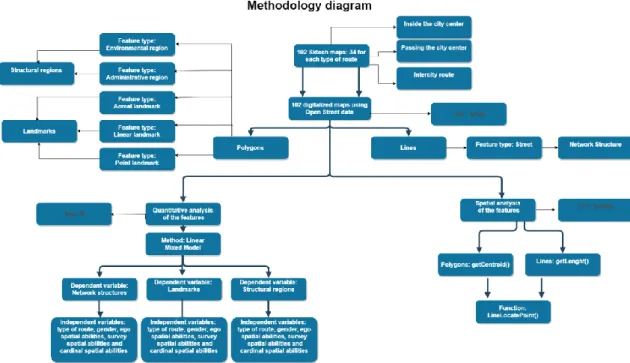
Figure 1: Methodology diagram ... 17

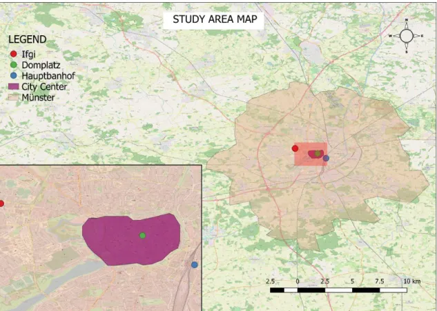
Figure 2: Estudy area ... 19

Figure 3: Orientation features classification ... 23

Figure 4: Boxplot with the total of features included in each type of route ... 27

Figure 5: Location of features along the route in intercity routes ... 32

Figure 6: Location of structural regions along the route in intercity routes ... 32

Figure 7: Location of features along the route in routes going to the city center ... 33

Figure 8: Location of structural regions along the route in routes going to the city center.. 33

Figure 9: Location of features along the route in routes inside the city center ... 34

Figure 10: Location of structural regions along the route in routes inside the city center ... 34

TABLE OF TABLES

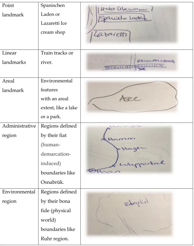
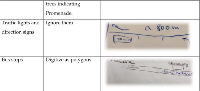
Table 2: Rules for digitalization ... 22

5

1. Introduction

During the last decades, the role of geographic information has changed. Nowadays, many technologies and digital applications make use of geographic data. Through the processes of digitalization, geographic information systems have expanded throughout the world and impacts in different areas. GIS technology provides numerous

outcomes, from digital cartography to GPS devices.

Advances on these technologies, such as analyzing data faster or more efficiently, are coming up every day. Of course, they are essential, but sometimes an important point is forgotten, how people perceive this information. To move from the real world to the digital model of reality, procedures related to the observation and description of the environment are needed for data collection.

Accordingly, Human-Computer Interaction increased notoriety. It brings together the interdisciplinary field of geographic information science, computer science, and

cognitive science. It focuses on the advancement of GI software using similar strategies to the human brain, to improve the interaction between human and computers.

For this reason, spatial cognition became important in the conceptualization of reality. It allows us to transmit spatial information in more effective ways, taking into account that different persons will differ in their cognitive abilities. Researchers have been interested in decades in the perception of the environment, inferring that it is not objective (Navarro & Rodríguez, 2008). The previous experiences that each has had, influence on how places and routes are saved in our memories and how people build their cognitive maps (Ishikawa and Montello, 2006). Associating those locations along with the routes stored in our minds forms what is called cognitive maps (Hegarty et al., 2006).

Spoken and written language and drawings are externalizations of the human mental representations (Richter & Winter, 2014). In previous studies, sketch maps have represented a handy tool for measuring and evaluating spatial knowledge and how people understand the space. Psychologists have widely used sketch maps, researchers

6

in the social sciences, urbanists, and geographers (Navarro & Rodríguez, 2008). They are an externalization of an individual’s mental images of the environment (Jan, Schultz, Schwering, & Chipofya, 2015) which originate from cognitive maps (Krukar, Schwering, & Anacta, 2017).

Each person uses different techniques to retrieve the necessary information from their brains to create sketch maps (Lynch, 1960). Because of this, there are various

distortions and modifications. Even so, they contribute precious information on people´s spatial knowledge. The spatial knowledge concept consists mainly of three significant components: landmark knowledge, route knowledge, and survey

knowledge (Aginsky et al., 1997).

Previous studies usually focus on two perspectives: look for general landmarks

candidates or dig on the reasons that make a landmark important for some individuals and not for others.

In the study carried out by Kyritsis et al. (2014), the reasons that influence these disparities, are distributed in two main groups: biological or environmental. On one hand, biological reasons such us participant´s age (Vázquez & Noriega Biggio, 2010), gender (Linn, Marcia & Petersen, 1985) and spatial orientation skills (Kyritsis, Gulliver, & Morar, 2014). On the other hand, environmental such as changing seasons and the day/night cycle (Krukar, Schwering, & Anacta, 2017) or the type of route where they are located (Anacta, Schwering, Li, & Muenzer, 2017).

1.1 Research Questions

What are the different type of features in people´s sketch maps for different types of routes in familiar environments?

What are the different relation of features in people´s sketch maps for different types of routes in familiar environments?

7

1.2 Hypotheses and objectives

My first hypothesis expects that people include will include different features when drawing sketch maps for different types of routes.

My second hypothesis expects different relations of features in people´s sketch maps for different types of routes.

To answer previous questions, the following objectives have been established:

1. Examine the type of features, and relations people would include in sketch maps. 2. Investigate the reasons for the differences. Find out through qualitative and quantitative analysis of the data, if they are more related to environmental or individual reasons.

3. Draw conclusions based on the results obtained from the different analysis that help future researches.

8

2. Related work

After a lot of literature review has been done, the main factor is how the information is stored in people´s brains and how they retrieve this information once they need it. In the next points, I will cover the topics need it to understand the fundamental ideas of the thesis. As people act in the environment, they perceive the surrounding space and acquire knowledge about it. (Ishikawa & Montmello, 2006). When humans explore space they not only perceive it but they build up a mental representation of it (Tversky, 1993).

2.1 Spatial cognition

Spatial cognition refers to the acquisition, organization, utilization, and revision of knowledge about spatial environments. It relates to how human beings deal

with issues concerning relations in space, navigation, and wayfinding (Sjölinder, 1998). Spatial cognition research includes several cognitive functions, covering mainly three topics (Denis, 2017):

- How humans acquire geographic information and how they experience the

surrounding space. Spatial cognition allows us to transmit the information in more effective ways taking into account that the perception of the environment is not objective (Navarro & Rodríguez, 2008) and it is influenced by our previous experiences.

- How humans represent and communicate geographic information. Externalizing mental spatial representations always involves cognitive transformation processes, which include invoking parts of the mental image and encoding it into a chosen modality (Richter, 2013).

- Thirdly, how humans use geographic information. People make use of the spatial data they have stored in their brains for different purposes. They can be classified mainly in two groups, wayfinding, and navigation and places design with a particular purpose.

A recurrent topic is the evolution of spatial abilities over time. It is hypothesized that spatial abilities were more important in prehistoric times. However, each lifestyle demands some abilities more than others. On the one hand, hunting people present good visual discrimination which was the basis of ancient life. On the other hand, modern humans

9

developed new abilities such as language and new spatially based abilities, increasing the aptitudes of handling information with spatial content (Ardila, 1993).

2.2 Spatial learning & spatial knowledge

There are two ways for acquiring spatial knowledge, either through real-world

navigational experience (primary spatial knowledge) or from memory for locations that are obtained from maps (secondary spatial knowledge) (Sjölinder, 1998).

People’s surroundings representations can be very different since they are acquired

through our daily life activities. According to Barbara Tversky (1993), we can say that there are two ways of creating mental representations of the surroundings, by gradually

acquiring elements of the world or acquiring disparate pieces of the environment. Previous research (Montmello,1998), classified the process of knowledge acquisition in two: the dominant and the alternative framework.

The dominant framework was introduced by Siegel and White (1975). They described the process of acquiring spatial knowledge as continuous: landmark, route and survey knowledge are learned in order respectively.

When it comes to exploring a new environment, people start scanning it to identify and locate places and important objects. Landmark knowledge is knowledge about the

identities of discrete objects or scenes that are salient and recognizable in the environment (point features). After, they continue structuring their knowledge to create relationships between different objects. Route knowledge consists of sequences of landmarks and associated decisions (line features). Finally, other spatial information is added to the prior knowledge and thus have a general vision of the environment. Survey knowledge

represents distance and directional relationships among landmarks, including those out of the route, introducing metric survey information. These three types of knowledge are interrelated to consolidate space knowledge.

The alternative framework was introduced by Montmello (1998). In this case, it is considered that there is no stage in spatial knowledge where only specific features as landmarks or routes are remembered. Also, metric information appears at the first exposure to a place, increasing all the types of knowledge with exposure and familiarity.

10

2.3 Mental spatial representation

The different representations of the combination of spatial knowledge are defined as a cognitive map (Tolman, 1948) or cognitive collage (Tversky, 1993).

The term cognitive map (Tolman, 1948) was introduced to describe how rats, and therefore humans, behaved in the environment. It includes both the information extracted from the environment and how the subjects recover spatial knowledge elements and manage to represent them so that they have meaning for other people. In this case, people´s cognitive representations have a map structure.

In cognitive collages, the important information is not organized in one simple cognitive structure and it can be in represented in different ways. They lack the coherence of maps but do contain figures, partial information, and different perspectives (Tversky, 1993). It is important to highlight that these mental representations of the environment are not a perfect depiction of the reality and they may introduce incoherent parts and distortions. (Kray, 2003).

2.4 Sketch maps

The two main communication modes for externalizing mental spatial representations are, on the one hand, spoken or written language and on the other, hand graphical

configurations as sketch maps (Richter & Winter, 2014).

As said before, the sketch maps are influenced by cognitive impacts and introduce distortions. However, sketch maps are handy to convey spatial knowledge. Since most people can draw maps to communicate their spatial knowledge, sketch maps called the externalization of cognitive maps, are used frequently to measure cognitive maps (Wang & Schwering, 2015).

Previous studies (Anacta et al., 2018), worked with sketch maps created when the

participants were conducted to give route instructions. Along with the route, participants included all the information they considered necessary for someone unfamiliar to navigate in a specific environment.

Two types of data compose sketch maps, quantitative (the features itself) and qualitative (the topological relations between spatial objects).

11

2.4.1 Features

Landmarks are defined as “geographic objects that structure human mental representations of space” (Richter & Winter, 2014). They are essential elements for acquiring spatial

knowledge in an unfamiliar environment and maintain orientation. Most people rely on landmark information when asking for giving route directions as this makes it easier for them to remember.

Besides the existence of landmarks in route instructions itself, the location of these

landmarks has also been widely studied. (Anacta et al., 2018). In this direction, landmarks are classified into two groups, global and local landmarks. Local landmarks are visible features located either along the route or at decision points where a turning action has to be made. Global landmarks, on the other hand, refer to distant landmarks that are visible or non-visible located off the route. (Anacta, Schwering, Li, & Muenzer, 2017). It is known that human-generated route instructions consist of mostly local landmarks (Raubal & Winter, 2002).

2.4.2 Relation of features / Spatial location along the route

Although there are plenty of wayfinding studies investigating landmarks at decision points, the location of landmarks along the route has been less investigated. Besides, previous studies on this topic have not come to a common conclusion about their

position along the route. While some researchers concluded that there were more

landmarks included at the end of the route in sketch maps (Brosset, Claramunt, & Saux, 2008), others couldn´t find this outcome. (Lovelace, Hegarty, & Montello, 1999). Previous researchers studied the distribution of local landmarks along the route with relation to the length of the route differentiating three types of routes (Anacta et al., 2018). While in two types of routes, two peaks with a high amount of features were found (at the beginning and the end of the route), in the third type of route most of the

12

landmarks are located just at the end of the route. The frequency of landmarks in the middle part of the route also varies in the different type of routes.

2.5 Possible reasons for the differences in sketch maps

Previous research analyzed the individual differences in spatial abilities but also examined the effects of biological and environmental factors influencing this process.

Some of the biological factors studied previously are age, gender, and spatial strategies performance; environmental factors as the type of route.

2.5.1 Gender

In our culture, there are many gender stereotypes related to spatial skills and some of them are true. Although gender differences are found, the magnitude is small. There are

differences found between genders in several tasks, and it could be biologically based (Kimura, 1992) or explained by the course of human evolution.

Previous research (Cutmore et al., 2000) discovered that males prefer to solve navigation problems by using survey strategies and knowledge of cardinal directions. On the contrary, females use more route descriptions.

It is also ascertained, better performance of men in map reading, mentally rotating figures (Bjorklund, 1995) or spatial perception (Linn, Marcia & Petersen, 1985) which could have improved by hunting and the use of weapons. Women outperformed men on objects and location memory tasks, probably influenced by the traditional role of the women to stay at home and take care of the children. (Cutmore et al., 2000).

13

2.5.2 Spatial strategies performance

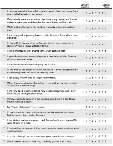
Even though many spatial skills have been intensively investigated, the cognitive skills used in navigating the environment have received less attention. It is believed that individuals who aced at visual-spatial tasks perform better on navigation tasks since they also require collection and deal with visual-spatial information. (Cutmore et al., 2000). To find out the spatial strategies that each person adopt, Stefan Münzer and Christoph Hölscher, created in 2010, the questionnaire “Fragebogen Räumliche Strategien FRS“ in German. The English translation is “Questionnaire on Spatial Strategies English-FRS.” It is a self-report measuring of spatial strategies. It consists of a set of 18 questions that refer to different spatial strategies used by the participants to orient themselves and locate features in their minds. All the answers have a positive value. It comprises three scales:

- “Global self-confidence, related to egocentric strategies.“ Egocentric represents the location of objects in space relative to the person itself (left-right, front-back, up-down). The questions number 1, 4, 5, 8, 10, 12, 13, 14, 15 and 18 refer to this scale.

- “Survey strategy.“ (See 2.2) .

The questions number 2, 3, 7, 9, 11 and 16 refer to this scale.

- “Knowledge of cardinal directions.“ Participants use cardinal directions (North, South, East, and West) to orient themselves in the environment.

The answers to questions number 6 and 7 refer to this scale.

2.5.3 Environment

The description of an environment varies with the people perspective and with the characteristics of the space. In previous research was affirmed that the different physical environments where people influence the type of features they include in route sketch maps. Furthermore, it was discovered (Schwering et al. 2013) that the relevance of global landmarks varies depending on the relation they have with the route. It was stated (Anacta, Schwering, Li, & Muenzer, 2017) that the city center was the most prominent

14

global landmark people use for orientation. However, if the person is navigating within a specific region, such as the city center, it is less probable that this region would be

mentioned. On the contrary, if the route starts outside the region or goes from city to city, it is more likely that region global landmarks are included.

Following this approach, a couple of studies (Anacta et al., 2016; Anacta, Schwering, Li, & Muenzer, 2017) made a distinction creating three different scenarios to evaluate if the features and the relations included by participants were different by route. They investigated local landmarks mentioned in three routes using a different mode of

transportation regardless of the route choices of participants and where the landmarks are concentrated in the entire route. For this, they used the city center as the main point of the study, choosing three routes and specifying the mode of transportation:

- Route 1: Going through the city center (within the city) using a bike. - Route 2: Going past the city center (across the city) using a bike. - Route 3: Between two cities (intercity route) using a bike and car.

The study concluded, on the one hand, that local landmarks along the route were drawn in sketch maps for every route. On the other hand, global, regional landmarks were included in all the routes representations, with more presence in intercity routes, longer routes where a car is selected as a mode of transportation. They support the participant´s

orientation. This shows that scale and mode of transportation lead also to a different use of global landmarks (Schwering, Li, & Anacta, 2014).

15

3. Methodology

The study is based on the collection of sketch maps. The maps provide spatial data that is analyzed to meet the hypothesis and answer the research questions.

In the hypothesis section, two concepts are introduced, features and relation of features. Besides, it digs on their differences and the possible reasons for these differences, environmental or individual.

To find out, if the features included are different for each kind of route, quantitative analysis will be carried out, using a linear mixed effects model.

The second hypothesis covers spatial relations. Therefore the data needs to be digitized. Subsequently, spatial analysis is applied, where are the features located along the line. The third hypothesis concern the reasons of the previous differences. The results of the two analysis will show if the environment influences these differences. The spatial strategies data together with the gender data collected will help us discover if instead, the reasons biological.

16

3.1 Participants

A total of 35 people participated in the experiment (21 M, 14 F). One user was excluded because the maps were not qualified for the study. The final participants were 34 (20 M, 14 F). The age will be a parameter in my research; so teachers, students or workers are all eligible. The average age of all participants is 28,97 years (M=28.97, SD=8,57). The requirement that participants must meet is to have lived in the city of Munster or surrounding areas for a minimum of six months, enabling them to be familiar with the study area (Anacta, Schwering, Li, & Muenzer, 2017), and all the locations asked to be drawn in the sketch maps.

This project includes real people. Therefore specific ethical considerations were taken into account. Before the experiment, all the participants signed a consent form. It stated that no data would be used individually and it would be only processed in aggregate. It also specified that users had the right to quit the study at any point. The university´s ethics commission supported the whole process.

3.2 Research design

The method consists of an empirical collection of sketch maps for different types of routes. The task was designed to last from half an hour to one hour; some participants finished in 20 minutes while others continue more than an hour to complete the assignment. To begin with, the necessary information was provided, and they were directed to create sketch maps, as detailed as possible, solely from memory. Three A4 paper sheets were distributed, one for each sketch map they had to generate. There were no restrictions and no specific time to complete the task. A total of 105 maps were collected.

Previously, they had to sign a consent form and to finalize, fill up a questionnaire. The whole research was created in English and German, according to the language each participant preferred.

17

3.3 Study area

Figure 2. Study area.

The study area is the city of Münster (Germany). The area was selected as the

experiment location by the proximity and familiarity to both the participants and the researcher. Before collaborative acceptance, all the candidates confirmed they were familiar with the area.

The three different maps correspond to three different environment/routes used in the experiment. The city center is used as the axial point for the study. The participants were asked to provide three maps with all the information needed to get from one place to another.

The first route is mainly inside the city center. It goes from the cathedral (Domplatz) to Ifgi (Institute for Geoinformatics).

The second route is going to the city center. It goes from Münster train station (Hauptbahnhof) to Ifgi.

The third route is an intercity route. In this case, it is different for each participant as it goes from their hometown to Ifgi.

18

3.4 Research procedure

In the study, the selected participants were asked to bestow route descriptions to a friend unfamiliar with the area. The method of transport was also specified. For the routes within and going to the city center, the transport indicated was via bicycle meanwhile in the intercity route, the means of transport was by car as this is a longer route that connects two cities. No additional details were given.

The order of the tasks (maps) was randomized since it may influence the results.

3.5 Spatial strategies questionnaire

Ensuing the drawing of sketch maps, a spatial strategies test was given. The participants had to evaluate the spatial strategies used by themselves in several situations. Also, age and gender were collected as additional information.

The spatial strategies questionnaire used in the research is “The Questionnaire on Spatial Strategies English FRS”(See 2.5.2). The answers to the questions give a score related to each one of the scales. These scores will be further needed in the research.

3.6 Data classification

A previous classification scheme created by Heinrich Löwen was used as the starting point to classify the features drawn. This classification was applied to my quantitative analysis of the features.

Feature type Explanation and examples

Sketch´s Examples Street Line features

like

19 Point landmark Spanischen Laden or Lazaretti Ice cream shop Linear landmarks Train tracks or river. Areal landmark Environmental features with an areal extent, like a lake or a park. Administrative region Regions defined by their fiat (human- demarcation-induced) boundaries like Osnabrük. Environmental region Regions defined by their bona fide (physical world) boundaries like Ruhr region.

20

3.7 Data digitalization

To convert hand-drawn maps into digital data, the same classification scheme created by Heinrich Löwen was followed. It establishes specific rules for adding or not features to the digitized maps. To develop this task, QGIS was the software used, and

OpenStreetMap was used as the as the base map data.

A total of 102 maps where digitized. Each participant had three folders, each one for a type of route. Each map/folder was composed of two shapefiles (lines and polygons) corresponding with landmarks and streets.

Features Rules and examples Sketch´s Examples Not identifiable

features

Do not digitize

Roundabout Do not digitize unless it is a decision point or has a name like

Ludgeriplatz.

Digitized as a polygon. Junctions Digitize when they are

used as landmarks like Coestfelder Kreuz. Streets without

names but when it is clear which street they are by the drawing

Digitize

Style elements Ignore them unless they imply a precise meaning. They are not digitized, but their sense is taken into account. Example:

21

trees indicating Promenade.

Traffic lights and direction signs

Ignore them

Bus stops Digitize as polygons.

Table 2. Rules for digitalization.

3.8 Data analysis

The objective was to analyze what features and relations of features people include in sketch maps depending on the type of route they are allocated.

First, the drawn features were analyzed by six types, as classified in the point 3.6.2. Later, to make more meaningful the data analysis, I grouped the previous six type of features into three categories. In this case, the “Classification scheme for orientation information in wayfinding maps” (Löwen, Krukar & Wintel, 2018) was applied. It classifies all the orientation features on a map in three groups, regardless of their role or location. The three types are landmarks, network structures, and structural regions as shown in the diagram below.

22

I implemented two types of analysis, a quantitative analysis of the features and a spatial analysis of these.

3.8.1 Linear mixed effects model

For the qualitative analysis of the features, I performed a linear mixed effects model. As explained previously, the features are divided into three groups: streets, landmarks, and regions. All these features are quantified and analyzed.

To study the relations in our data, I used a linear mixed effects model. We followed the tutorial “Linear models and linear mixed models in R” by Bodo Winter (2016).

It is an extension of simple linear models to allow both fixed and random effects. In the linear model, the world is divided into things that we understand (the fixed effects) and things that we don´t understand or can’t be controlled(e).

In our model, we add random effects to the fixed effects. The random effects are the structure of the “understandable term”(e).

In our case, the model crated is:

model <- value ~ environment + gender + survey + ego + cardinal + (1|Participant) ● Value corresponds with the number of features drawn. We do this three times, for streets, landmarks, and regions. In this example, we are using the street features. ● Environment corresponds with the type of route/environment: starting in the city center, going to the city center or from one city to another.

● Gender corresponds to male and female.

● Survey corresponds with Survey spatial strategies. ● Ego communicates Egocentric spatial strategies ● Cardinal corresponds with Cardinal spatial strategies.

● (1|Participant) is the random effect and it says there is more than one participant. The formula outlines whether the streets people include in sketch maps are influenced by the environment, high survey spatial strategies, high ego spatial strategies or cardinal spatial strategies.

23

To see this, a null model is created without each one of these characteristics. The idea is to see if the differences in the result are significant without each variable.

The comparison is made with the ANOVA test that compares the initial results with the results without variables indicated variables.

Verifying if the environment influences the network structures people include in sketch maps.

model_null <- (value ~ gender + survey + ego + cardinal + (1|Participant) anova(model_null,model)

Verifying if the gender influences the network structures people include to sketch maps.

model_null <- (value ~ environment + survey + ego + cardinal + (1|Participant) anova(model_null,model)

Checking if the spatial survey strategis influence the network structures people include in sketch maps.

model_null <- (value ~ environment + gender + ego + cardinal + (1|Participant) anova(model_null,model)

Certifying if the spatial ego strategies influence the network structures people include in sketch maps

model_null <- (value ~ environment + gender + survey + cardinal + (1|Participant)

anova(model_null,model)

Corroborating if the cardinal spatial strategies influence the network structures people include in sketch maps.

model_null <- lmer(value ~ environment + gender + survey + ego + (1|Participant)

24

This same structure is repeated two times, for landmarks and structural regions.

3.8.2 Spatial distribution of the features along the line

The centroid was calculated for each polygon, and the total length was calculated for each line.

Then, we reached the main point of the analysis, the function lineLocatePoint().

The returned value indicates how far along this linestring you need to transverse to get to the closest location where this linestring comes to every specified point.

It returns distance along the line, or -1 on error.

It gives the point along the line corresponded with the closest distance from each centroid to the line.

Once all the values along the line have been established, we normalize the line length to get the values in percentage.

The same steps are followed for the maps in the other two routes, within the city center and going to the city center.

To end, I carried out the same analysis just with structural regions to see if the behaviors differ for the different type of features.

25

4. Results

To answer the research questions, the results of the previous methodology section, are divided into three main parts:

1. Type of features included in each type of route.

2. The significance of the type of route, gender and the spatial strategies on the features included.

3. The location of features and the structural regions along the route. To make easier to comment on the results, the routes will be specified as:

- The route starting in the city center: Route 1. - The route going to the city center: Route 2.

- The intercity route, from one city to another city: Route 3. The raw data can be found in the appendix.

4.1 Type of features included in each type of route.

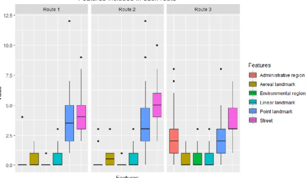
Figure 4. Boxplot with the total of features included in each type of route.

Looking at figure 4, we see how the streets and point landmarks are the most

26

There is a median of 4 streets included in route 1 and 5 in route 2.

25% of the people included more than 5 streets, and other 25% added less than 3. The variation is considerable, and streets, as well as point landmarks, are very sensitive to outliers. This is explained by the different familiarity of each participant. The most significant variances correspond to the participant that was living in Münster for the most prolonged period, and we can see how this might have influenced the features included.

In route 3, there are no outliers and all the participants introduced in between 1 and 7 streets.

The behavior in point landmarks is similar, in route 1 and 2, the medians are 4 and 3 respectively; in route 3 it decreases to 2. The maximum number of features represented excluding outliers are also higher in route 1 and 2. There are outliers in every route for the same reason as explained before.

Similar amounts of areal landmarks and linear landmarks are represented in all routes. 75% of the participants included between 0 and 1 features. The maximum number of features represented excluding outliers are 2.

In structural regions, there are again differences in between route 1 and 2 and route 3. In route 1 and 2, environmental regions are usually not included (except outliers that included one). In route 3, the participants included in between 0 and 1 environmental features, the maximum amount of features included without outliers is 2.

The most significant difference is found in the administrative landmarks, while in route 1 and route 2 are vaguely represented, mean of 0 with outliers including 2, 3 and 4; in route 3 are the most represented features. The mean is located in 2 administrative

landmarks, and 75% of the participants included until 3. The maximum amount of

features included without outliers is 6. Outliers included up to 8 administrative landmarks.

The previous results show that there are differences in the features people include in sketch maps. Additionally, the graph reveals there are differences in the features included in each type route. Nevertheless, with these results, we can say there are differences, but there is no statistical evidence, it will be concluded in the next section with the linear fixed effects model results.

27

4.2 The significance of the gender, type of route and spatial

strategies on the features included.

As explained before, the features included are divided into three groups to simplify the results.

I performed a linear mixed effects model and an ANOVA test. The outcome helps me to find out the significance of the results. The complete results can be seen in appendix B.

I created an alternative hypothesis and a null hypothesis. With the null hypothesis, I assume that there are no differences excluding a variable. The alternative model would be true in the case that the hypothesis is false. The ANOVA test gives the significance of the variable removed, in the alternative model. For this, the chi-square goodness of fit test is performed. Based on the chi-square statistic and the degrees of freedom, we determine the P-value. The P-value is the probability that a chi-square statistic having 2 degrees of freedom is more extreme than the specific number given by the model. The p-value is represented as a number between 0 and 1 and interpreted as follows:

 ≤ 0.05 indicates the likelihood of the values I get show no difference is below 5%.

 > 0.05 means the null hypothesis makes a considerable difference in the alternative hypothesis.

 Values very close to 0.05 may indicate a tendency in both directions.

Following these statistics, it is concluded that:

Results for network structures

Network structures are affected with significance by the type of route and egocentric spatial strategies.

- The type of route affected network structures X2(1) =14.15, p=0.00085. Intercity routes decreasing it by about 0.62 +- 0.30(standard errors). Going to the center routes increasing it by about 0.56 +- 0.30(standard errors).

28

Route going to the city center (M=4.88, SD=1,79) Intercity route (M=3.71, SD=1,64)

- Egocentric spatial strategies affected network structures X2(1)=5.11, p=0.02381, increasing it by about 0.085 +- 0.37(standard errors).

Gender, Survey spatial strategies, and Cardinal spatial strategies didn´t affect the number of street networks with significance.

- Gender affected network structures X2(1)=2.59, p= 0.1079, increasing it by males by about 0.71 +- 0.4 (standard errors).

- Survey spatial strategies affected streets X2(1)=1.46, p=0.23, decreasing it by about 0.047 +- 0.39(standard errors).

- Cardinal spatial strategies affected streets X2(1)=0.76, p=0.7839, decreasing it by about 0.025 +- 0.09(standard errors).

Results for landmarks

Landmarks are affected with significance by type of route and gender.

- The type of route affected landmarks X2(1)=5.154, p=0.076. Intercity routes decreasing it by about 0.62 +- 0.27(standard errors). Going to the city routes decreasing it by about 0.030 +- 0.27(standard errors).

Route starting in the city center (M=1.61, SD=2,13) Route going to the city center (M=1.58, SD=2,14) Intercity route (M=1.07, SD=1,41)

- Gender affected landmarks X2(1)=3.29, p=0.06989, decreasing it male gender by about 0.45 +- 0.25(standard errors).

Egocentric spatial strategies, Survey spatial strategies, and Cardinal spatial abilities didn´t affect the number of landmarks with significance.

- Egocentric spatial strategies affected landmarks X2(1)=0.60, p=0.442, increasing it by about 0.015 +- 0.02(standard errors).

- Survey spatial strategies affected landmarks X2(1)=0.37, p=0.55, decreasing it by about 0.013 +- 0.02(standard errors).

29

- Cardinal spatial strategies affected landmarks X2(1)=0.02, p=0.88, decreasing it by about 0.54 +- 0.05(standard errors).

Results for structural regions

Structural regions are affected with significance by type of route.

- The type of route affected regions X2(1)=54.63, p=1.374e-12. Intercity routes increasing it by about 1.250e+00 +- 1.792e-01(standard errors). Routes going to the city center decreasing it by about 4.412e-02 +- 1.792e-01(standard errors). Route starting in the city center (M=0.09, SD=0,51)

Route going to the city center (M=0.13, SD=0,49) Intercity route (M=1.34, SD=1,70)

Gender, Egocentric spatial strategies, Survey spatial strategies, and Cardinal spatial abilities didn´t affect the number of structural regions with significance.

- Gender affected regions X2(1)=0.20, p=0.65, increasing it male gender by about 7.494… +- 1.657e-1(standard errors).

- Egocentric spatial strategies affected regions X2(1)=0.53, p=0.11, increasing it by about 2.141e-02 +- 1.343e-02 (standard errors).

- Survey spatial strategies affected regions X2(1)=0, p=0.99, increasing it by about 8.977e-05 +- 1.4393-e02 (standard errors).

- Cardinal spatial strategies affected regions X2(1)=0.811, p=0.37, decreasing it by about 3.094-e02 +- 3.432-e02 (standard errors).

Even though p-value itself doesn’t mean anything, it is a way to summarize the statistical results explained previously. We see how the type of route is the only reason influencing all the type of features.

TOTAL PARTICIPANTS P.VALUE RESULTS

TYPE OF ROUTE EGO SURVEY CARDINAL GENDER

NETWORK

STRUCTURES 0,00085 0,02381 0,227 0,7839 0,1079

LANDMARKS 0,076 0,442 0,5452 0,8808 0,06989

STRUCTURAL REGIONS 1,374 e-12 0,112 0,995 0,3768 0,65

30

4.3 The location of features and the structural regions along

the route.

Figure 5. Location of features along the route in intercity routes.

Figure 5 shows the location of the total features along intercity routes at a normalized distance scale from 1 to 100. The graph reveals there are more landmarks at the beginning and the end of the route.

In the middle parts of the route, the frequency is much smaller with a maximum of between 5 and 10 features.

Figure 6. Location of structural regions along the route in intercity routes.

Figure 6 shows the location of structural regions along intercity routes at a normalized distance scale from 1 to 100. In this case, the maximum frequency of structural regions is located at the beginning of the route. This shows that structural regions are not noticeably represented at the end of the route when participants go from one city to another. At the same time, we see that most of the features represented in this type of route are structural regions.

31

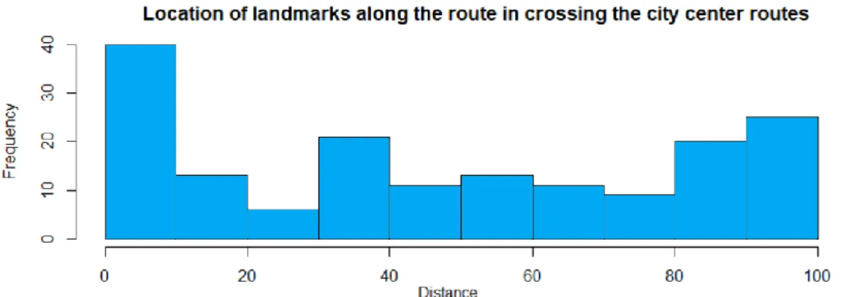
Figure 7. Location of features along the route in routes going to the city center.

Figure 7 shows that in routes going to the city center, the features are more regularly distributed along the line. Again, the route is represented in a normalized distance scale from 0 to 100. The maximum frequency of features is located at the beginning of the route, while in the rest there are lower frequencies with values between 10 and 20 features, while at the beginning they go up to 40.

Figure 8. Location of structural regions along the route in routes going to the city center. Figure 8 demonstrates that structural regions are little represented in routes going to the city center. The highest frequencies are located again at the beginning and the end of the route, with the highest concentration of structural regions at the beginning, with 7 features.

32

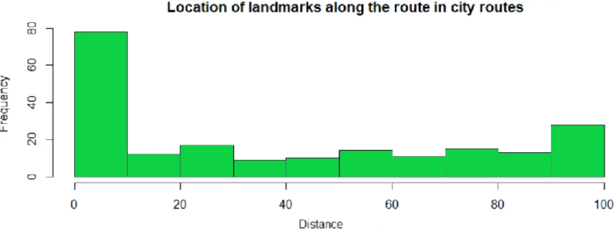
Figure 9. Location of features along the route in routes inside the city center.

Figure 9 demonstrates a concentration of features again at the beginning of the route, even more, accentuated than in the previous figures.

Figure 10. Location of structural regions along the route in routes inside the city center. Figure 10 shows that structural regions are concentrated mainly, at the beginning of the route; and in second place, at the end of the route. Again, there is a total absence of features in the middle of the route.

33

5. Discussion

The importance of landmarks in route descriptions has been widely investigated (Krukar, Schwering, & Anacta, 2017). As well the influence of the environment and mode of transportation on landmarks was studied previously (Schwering, Li, & Anacta, 2014; Lovelace, Hegarty, & Montello, 1999). In the study performed by Schwering et al., they showed that in longer routes, where transportation by car is required, the number of global landmarks increases. This is also evident in my study. The environment interferes in the different location of landmarks, showing differences in all the route types. Especially in intercity routes that are longer and, therefore, require a car as a mode of transportation, there are more structural regions (usually used as global landmarks). The reason can be, that on longer routes, the participants include structural regions for orientation purposes. However, it is worth pointing out that there are differences in all the features included for the three routes.

In the study performed by Lovelace et al., they concluded that the length of the route did not influence the number of landmarks included. In general, route 2 included the highest amount of features. While in my study, the length of the route did influence the existence of structural regions, route 1 and 2 also included more features. This can be explained since in the city center there are more prominent objects considered

landmarks, such as shops or restaurants.

Also, the influence of gender in spatial abilities such as mentally rotating figures was investigated previously (Linn, Marcia & Petersen, 1985). They concluded that female outperformed male on objects and location memory tasks. In my work, it was found out that gender affects the amount of remembered landmarks: They are introduced more often by females than by males. Although this can be explained by the better performance of female on objects and location memory tasks, it should be considered that there are no significant differences in the representation of street networks or structural regions.

Previous studies have also investigated the spatial distribution of local landmarks along the route in route descriptions (Anacta et al., 2018) concluding that their spatial distribution differs along the route and is depending on the type of route. Concretely, within the routes 2 and 3, there are more local landmarks at the beginning and the end;

34

and in route 1, there is a single peak with more landmarks at the end of the route. In contrary, this distribution is different in my study. Within all the three routes, there is the same distribution, a peak with more features at the beginning of the route and a second peak at the end of the route. These results match with another study (Lovelace, Hegarty, & Montello, 1999) where the same spatial pattern is indicated. Including more landmarks at the end of the route is related to orientation purposes. When getting closer to the target point, the route could be more complex and therefore more information is needed for successful navigation.

35

6. Conclusions and Outlook

Navigation systems and location-based devices make continuous use of landmarks. Many studies have been performed to investigate the presence and location of landmarks in the route instructions.

In this paper, it was identified, on the one hand, how the type of route influences the presence of all the features. Especially, the structural regions, are much more frequently included in intercity routes. Besides, we see that streets and landmarks are more regularly often included in the three types of routes. Although, all landmarks exhibit changes in their spatial distribution patterns, which are influenced by the type of the route.

Furthermore, it was proved that the gender of the participants influences the landmarks they include, where females are drawing more features than males. Also, the Egocentric spatial strategies influence the number of network structures that people include.

Participants with a higher score in this spatial strategy include more features than others. On the other hand, for results with no significance, we do not have statistical evidence to reject the null hypothesis, which claims that survey spatial strategies and cardinal spatial strategies do not influence the number of features people include in sketch maps. In a nutshell, the type of route is the only reason that influences the three type of features, which is supporting our hypothesis.

Regarding the location of the features along the route, there is a common pattern found in the three types of routes: A peak with more features at the beginning of the route and a second peak at the end of the route. The only difference is, that in route 1 and 2 there is a total absence of structural regions in the middle part of the route, while within route 3 not (although there are also more at the beginning and the end).

For future work, it could be interesting to previously classify global and local landmarks and then study the distribution of them along the line in route instructions. It would also be helpful to investigate different levels of familiarity. The differentiation performed in this research could introduce some bias because it only takes into account if people are familiar or unfamiliar with the environment. Lastly, it is recommended to perform different spatial analysis of the features, such as the direction of the features in sketch maps.

This work provides benefit to ongoing researches on navigation and location-based devices focused on the automatic generation of landmarks for a specific route.

36

7. References list

1. Aginsky, V., Harris, C., Rensink, R., & Beusmans, J. (1997). Two strategies for learning a route in a driving simulator. Journal of Environmental Psychology, 17(4), 317-331

2. Anacta, V. J. A., Schwering, A., Li, R., & Muenzer, S. (2017). Orientation information in wayfinding instructions: evidences from human verbal and visual instructions. GeoJournal, 82(3), 567–583.

https://doi.org/10.1007/s10708-016-9703-5

3. Anacta, V., Li, R., Löwen, H., Galvão, M., & Schwering, A. (2018). Spatial

Distribution of Local Landmarks in Route-Based Sketch Maps: 11th International Conference, Spatial Cognition 2018, Tübingen, Germany, September 5-8, 2018, Proceedings (pp. 107–118). https://doi.org/10.1007/978-3-319-96385-3_8

4. Ardila, A. (1993). Historical Evolution of Spatial Abilities. Behavioural Neurology, 6(2), 83–87. https://doi.org/10.1155/1993/567986

5. Bjorklund, D. F. (1995). Children's thinking: developmental function and individual differences. Pacific Grove, Calif. Brooks/Cole Pub. Co.

6. Brosset, D., Claramunt, C., & Saux, E. (2008). Wayfinding in Natural and Urban Environments: A Comparative Study (Vol. 43).

https://doi.org/10.3138/carto.43.1.021

7. Cutmore, T. R. H., Hine, T. J., Maberly, K. J., Langford, N. M., & Hawgood, G. (2000). Cognitive and gender factors influencing navigation in a virtual

environment. International Journal of Human-Computer Studies, 53(2), 223–249. https://doi.org/10.1006/ijhc.2000.0389

8. Hegarty, M., Montello, D. R., Richardson, A. E., Ishikawa, T., & Lovelace, K. (2006). Spatial abilities at different scales: Individual differences in aptitude-test performance and spatial-layout learning. Intelligence, 34(2), 151–176.

https://doi.org/10.1016/j.intell.2005.09.005

9. Ishikawa, T., & Montello, D. R. (2006). Spatial knowledge acquisition from direct experience in the environment: Individual differences in the

development of metric knowledge and the integration of separately learned places. Cognitive Psychology, 52(2), 93–129.

37

10. Jan, S., Schultz, C., Schwering, A., & Chipofya, M. (2015). Spatial Rules for Capturing Qualitatively Equivalent Configurations in Sketch maps (pp. 13–20). https://doi.org/10.15439/2015F372

11. Kimura, D. (1992). Sex Differences in the Brain. Scientific American, 267(3), 118-125. http://www.jstor.org/stable/24939218

12. Klippel, A., & Winter, S. (2005). Structural Salience of Landmarks for Route Directions. In A. G. Cohn & D. M. Mark (Eds.), Spatial Information Theory (Vol. 3693, pp. 347–362). Berlin, Heidelberg: Springer Berlin Heidelberg.

https://doi.org/10.1007/11556114_22

13. Kray, C. (2003). Situated Interaction on Spatial Topics (Dissertation). Saarland University, Saarbrücken, Germany.

14. Krukar, J., Schwering, A., & Anacta, V. J. (2017). Landmark-Based Navigation in Cognitive Systems. KI - Künstliche Intelligenz, 31(2), 121–124.

https://doi.org/10.1007/s13218-017-0487-7

15. Kyritsis, M., Gulliver, S. R., & Morar, S. (2014). Cognitive and Environmental Factors Influencing the Process of Spatial Knowledge Acquisition within Virtual Reality Environments: International Journal of Artificial Life Research, 4(1), 43–58. https://doi.org/10.4018/ijalr.2014010104

16. Linn, M. C. y A. C. Petersen (1985), “Emergence and characterization of sex differences in spatial ability: A meta-analysis”, Child Development (Vol. 56, pp. 1479-1498).

17. Lovelace, K. L., Hegarty, M., & Montello, D. R. (1999). Elements of Good Route Directions in Familiar and Unfamiliar Environments. In C. Freksa & D. M. Mark (Eds.), Spatial Information Theory. Cognitive and Computational Foundations of Geographic Information Science (Vol. 1661, pp. 65–82). Berlin, Heidelberg: Springer Berlin Heidelberg. https://doi.org/10.1007/3-540-48384-5_5

18. Löwen, H., Krukar, J., & Schwering, A. (2018). How should Orientation Maps look like?

19. Löwen, H., Schwering, A., Krukar, J., & Winter, S. (2017). Perspectives in Externalizations of Mental Spatial Representations. In A. Bregt, T. Sarjakoski, R. van Lammeren, & F. Rip (Eds.), Societal Geo-innovation (pp. 111-127). Cham: Springer International Publishing. https://doi.org/10.1007/978-3-319-56759-4_7

38

20. Lynch, K. (1960). The Image of the City. The M.I.T Press. https://doi.org/10.2307/427643

21. Montmello, D. R. (1998). A new framework for understanding the acquisition of spatial knowledge.

22. Navarro, O. E., & Rodríguez, U. (2008). Los mapas cognitivos o la adquisición de un

saber espacial como método de investigación social, 20.

23. Raubal, M., Winter, S. (2002). Enriching Wayfinding Instructions with Local Landmarks. In Egenhofer, M., Mark, D., eds.: GIScience '02 Proceedings of the Second International Conference on Geographic Information Science, pp.243-259

24. Richter, K.-F. (2007). A Uniform Handling of Different Landmark Types in Route Directions. In S. Winter, M. Duckham, L. Kulik, & B. Kuipers (Eds.), Spatial Information Theory (Vol. 4736, pp. 373–389). Berlin, Heidelberg: Springer Berlin Heidelberg. https://doi.org/10.1007/978-3-540-74788-8_23 25. Richter, K.-F. (2013). Prospects and Challenges of Landmarks in Navigation

Services. In M. Raubal, D. M. Mark, & A. U. Frank (Eds.), Cognitive and Linguistic Aspects of Geographic Space (pp. 83–97). Berlin, Heidelberg: Springer Berlin Heidelberg. https://doi.org/10.1007/978-3-642-34359-9_5 26. Richter, K.-F., & Winter, S. (2014). Landmarks: GIScience for Intelligent Services.

Springer International Publishing.

27. Schwering, A., Li, R., & Anacta, V. J. (2013). Orientation Information in different Forms of Route Instructions. In D.Vandenbroucke, B. Bucher & J. Crompvoets (Eds.), Short Paper Proceedings of the 15th AGILE International Conference on Geographic Information Science, Leuven, Belgium.

28. Schwering, A., Li, R., & Anacta, V. J. A. (2014). The Use of Local and Global Landmarks across Scales and Modes of Transportation in Verbal Route Instructions, 5.

29. Siegel, A. W., & White, S. H. (1975). The Development of Spatial Representations of Large-Scale Environments (Vol. 10). https://doi.org/10.1016/S0065-2407(08)60007-5

30. Sjölinder, M. (1998). Spatial Cognition and Environmental Descriptions. In Exploring Navigation: Towards a Framework for Design and Evaluation of Navigation in Electronic Spaces. Ed. Nils Dahlbäck. SICS Technical Report T98:01, March 1998, ISSN: 1100-3154, ISRN: SICS-T-98/01-SE

39

31. Tolman, E. C. (1948). Cognitive maps in rats and men. Psychological Review, 55(4), 189–208. https://doi.org/10.1037/h0061626

32. Tversky, B. (1993). Cognitive Maps, Cognitive Collages, and Spatial Mental Models. In A. U. Frank & I. Campari (Eds.), Spatial Information Theory A Theoretical Basis for GIS: European Conference, COSIT’93 Marciana Marina, Elba Island, Italy, September 19-22 (pp. 14–24). Springer Berlin Heidelberg.

https://doi.org/10.1007/3-540-57207-4_2

33. Vázquez, S. M., & Noriega Biggio, M. (2010). La competencia espacial: Evaluación en alumnos de nuevo ingreso a la universidad. Educación Matemática, 22(2), 65–91. 34. Wang, J., & Schwering, A. (2015). Invariant spatial information in sketch maps — a

study of survey sketch maps of urban areas. Journal of Spatial Information Science, (11). https://doi.org/10.5311/JOSIS.2015.11.225

40

A. Experiment in English: Consent form, tasks, and

spatial strategies test.

41 Figure A.2: Consent form second page.

Figure A.3: Task for route starting in the city center.

42 Figure A.5: Task for the intercity route.

43

B. Results of linear mixed effects model (4.2).

Figure B.1: Network structures model fixed effects.

Figure B.2: Network structures null model without gender.

44

Figure B.4: Network structures null model without survey spatial strategies.

Figure B.5: Network structures null model without cardinal spatial strategies.

45 Figure B.7: Landmarks model fixed effects.

Figure B.8: Landmarks null model without gender.

46

Figure B.10: Landmarks null model without survey spatial strategies.

Figure B.11: Landmarks null model without cardinal spatial strategies.

Figure B.12: Landmarks null model without environment.

47

Figure B.14: Structural regions null model without gender.

Figure B.15: Structural regions null model without egocentric spatial strategies.

48

Figure B.17: Structural regions null model without cardinal spatial strategies.

49

C. Data attached.

Experiment data

- The original data that was collected through the experiment. Location:

https://drive.google.com/drive/folders/1jqrwYPPVsY6zglIl2CXJ3lEOp0xv1k00 - The digitized version of the data.

Location:

https://drive.google.com/drive/folders/1wN1YzuCSOlEbre2KRbSc7QO4O5qb_u vU

Analysis

- The scripts that were written for the analysis of the data. Location: https://github.com/VanesaPerez/Master-Thesis