Proceedings of the Eighth European Conference on Underwater Acoustics, 8th ECUA
Edited by S. M. Jesus and O. C. Rodr´ıguez Carvoeiro, Portugal
12-15 June, 2006
MATCHED-FIELD TOMOGRAPHY USING AN ACOUSTIC
OCEANOGRAPHIC BUOY
Cristiano Soares 1 and S´ergio M. Jesus1
1SiPLAB-FCT, University of Algarve
Campus de Gambelas 8005-139 Faro
Portugal
e-mail: {csoares,sjesus}@ualg.pt
Abstract: The Acoustic Oceanographic Buoy (AOB) is a light acoustic receiving device that is being developed in the framework of a joint research project and tested during the Maritime Rapid Environmental Assessment (MREA) sea trials. One of the AOB’s application is in Matched-Field Tomography (MFT) when a reduced number of receivers is available in opposition to traditional systems used in tomography. One problem of chief importance in MFT is the degree of uniqueness of the problem’s solution which is highly dependent on the number of receivers and on the number of free parameters. This paper studies the possibility of using matched-field processors with reduced ambiguity levels in comparison to conventional processors with application to acoustic data collected during the MREA sea trials. Two aspects are investigated: (a) the choice of an explicit broadband data model, where the exploitation of the spectral coherence of the acoustic field is seen as a mean to reduce the ambiguity level of the cost function used in the optimization; (b) conventional and high-resolution methods based on the proposed broadband model are implemented and compared.
1. INTRODUCTION
Environmental inversion of acoustic signals for bottom and water column properties is being proposed in the literature as an interesting concept for complementing direct hy-drographic and oceanographic measurements for Rapid Environmental Assessment (REA) [1]. Today, REA is one of the most appealing fields of study for military applications. The objective of REA is to provide environmental nowcasts and forecasts accurate and efficient enough to support operational activity in any arbitrary region of the global coastal ocean, and to respond effectively to operational assessment requests on very short notice. MFT can bring interesting advances to REA as the result of acoustic inversions that can be
assimilated into ocean circulation models tailored and calibrated to the scale of the area under observation. To make Acoustic REA (AREA) operational, the hardware involved in the reception of the acoustic signals must be light and handy. AREA must also be able to assimilate a priori environmental knowledge such as seafloor properties, bathymetry and telemetry data like GPS positions and acoustic source depth. Another component, intimately linked to the inversion process, is a collection of techniques, coming from sig-nal and array processing, used to efficiently carry out parameter estimation. In order to respond to the above requirements, an innovative concept of AREA was proposed under a NATO Undersea Research Centre (NURC) Joint Research Project, named AOB-JRP, formally started in 2004 1. That concept included the development of water column and geoacoustic inversion methods being able to retrieve environmental true properties from signals received on a drifting network of Acoustic-Oceanographic Buoys (AOB). A proto-type of an AOB and a preliminary version of the inversion code, was tested at sea during the Maritime Rapid Environment Assessment’2003 sea trial (MREA’03).
This paper investigates the possibility of using matched-field processors with higher discrimination ability than that achieved by the conventional processor. A subspace based processor based on a broadband data model [2] is proposed and compared with a con-ventional processor. Both methods are applied to the MREA’03 data set for performing MFT with a sparse receiver array and their parameter estimation performance is com-pared. The quality of the model estimates is evaluated by means of source localization using large search bounds.
2. THEORETICAL BACKGROUND
2.1 The broadband model
A broadband data model for the acoustic data received at an L-receiver array can be written as a concatenation of narrow-band signals
Y = [YT(ω1), · · · , YT(θ0, ωk), · · · , YT(θ0, ωK)]T
= H(Z, θs, Θ)S + N (1)
in order to introduce, as much as possible, a common frame for the narrowband and broadband cases. The main objectives are to proceed into a generalization in terms of frequency band, and to account for the signals’ cross-frequency correlations. The matrix H(Z, θs, Θ) is the channel response matrix and is given as
H(Z, θs, Θ) = H(ω1, Z, θs, Θ) · · · 0k−1 · · · 0K−2 01 · · · H(ωk, Z, θs, Θ) · · · 01 0K−2 · · · 0K−k · · · H(ωK, Z, θs, Θ) , (2)
where the ωk, k = 1, . . . , K represent the K discrete frequencies of interest. 0k is a vector
with kL zeros. Each column relates to a frequency ωk. The channel matrix has KL rows,
and K columns. The vector S has random entries S(ωk). The vector N represents the
noise and has obviously the same notation as Y in (1). The cross spectral density matrix (CSDM) is given as CY Y = HCSSHH + σN2 I, where CSS = E[S SH] is the signal matrix.
1The AOB-JRP was jointly submitted by the the Universit´e Libre de Bruxelles, Belgium, SiPLAB at
University of Algarve and the Instituto Hidrogr´afico (IH), both from Portugal, and the Royal Netherlands Naval College (RNLNC), The Netherlands.
2.2 Broadband matched-field processors
The previous section has presented the broadband data model. This model is used as the basis for obtaining the two matched-field processors whose derivation will not be shown. The conventional Bartlett processor has the following expression:
PBart(θ) = tr[HH(θ) ˆC Y YH(θ)CSS] tr[HH(θ)H(θ)C SS] , (3)
and the subspace based method is given as [3] PMUSIC(θ) = tr[HH(θ)H(θ)C SS] tr[HH(θ) ˆΠ⊥H(θ)C SS] , (4)
where ˆΠ⊥ = ˆUNUˆHN is the signal subspace orthogonal projector. The columns of matrix
ˆ
UN are noise subspace eigenvectors of the sample CSDM ˆCY Y. Matrix CSS will be
assumed unknown and must be estimated together with the parameter vector θ. This is done by estimating the signal term of the CSDM using a subspace based approach first, and then the channel response is filtered out [4].
There is one important remark to be made: applying subspace based methods re-quires the number of signal realizations N to be greater or equal to KL is order to obtain full rank SDMs. For the A1 and A2 signals N is equal to 10, and for the A1double sig-nals N is equal 16. Thus, for accounting for the condition, K will be less or equal to 3, which might clearly be a too low number of frequencies. For allowing the use of a larger number of frequencies each processor will be implemented as an average over frequency aggregates. For the present study a coherence based optimization algorithm for chosing the frequencies was employed. The criterion used maximizes the ratio between the two first eigenvalues of a field-phase correlation matrix. Further development on this is out of the scope of this paper.
3. EXPERIMENTAL RESULTS
The MREA’03 sea trial took place off the west coast of Italy in the North Elba Island area, during June 2003 [5]. The data consists of 2 seconds duration LFM chirps on two frequency bands. The signals designated by “A1” and “A1double” are LFMs in the band 500 to 800 Hz; the signals designated by “A2” are LFMs in the band 900 to 1200 Hz. The experimental setup consisted of a towed acoustic source and a free drifting AOB with receivers at nominal depths of 15, 60, 75, and 90 m. However, the deepest receiver will not be considered in this study due to extremely poor SNR during most of the experiment. The distance between the source and the AOB varies between 1 and 9 km.
3.1 Data processing procedure
This section explains the general procedure that consists in:
1. Frequency selection by optimizing the coherence based criterion.
2. Full field inversion for all unknown environmental and focusing parameters such as those related to the receiver array (e.g. tilt and receiver depth).
3. Inversion validation by means of source localization with large bounds using esti-mated environmental models.
4. Reconstruction of the physical parameters of interest using only the environmental estimates validated in step 3.
For the inversions to be performed it will be assumed that all parameters of a three-layers environmental model are unknown. The search parameters are divided into water-column (two EOF coefficients), sediment (upper and lower speeds, density, attenuation, thickness), sub-bottom (speed, density, attenuation) and geometric parameters (receiver depth and array tilt). The geometric parameters are regarded as focusing parameters, since their values are not required after MFT procedure is finished. The parameter vector is coded in 68 bits which results in a search space size approximately equal to 2.95 × 10²⁰. To perform the search, a GA has been used. Given the density of the processed data along time and the nature of this study only a single population is taken for each time point, from which the best individual is taken.
3.2 MFT on the MREA’03 data set: performance comparison
Once an environmental estimate was obtained, one tool available for evaluating the per-formance of each processor on the different emission periods is the result of step 3 - source localization. After performing MFT, source localization along time was performed within ranges from 1 to 10 km, and depths from 1 to 110 m. Figure 1 shows the localization re-sults based on the MFT inversions performed. Successful localizations are marked with a
10 11 12 13 14 2 4 6 8 10 Time (Hours) Range (km) BB Bartlett 10 11 12 13 14 20 40 60 80 100 Time (Hours) Depth (m) BB Bartlett 10 11 12 13 14 2 4 6 8 10 Time (Hours) Range (km) BB MUSIC 10 11 12 13 14 20 40 60 80 100 Time (Hours) Depth (m) BB MUSIC
Fig. 1 Source localization as a MFT validation step. True location is given by the red curve in the background. The gray curve with circles are the source localization results. The black asterisks indicate the successful localizations. The emission periods of the A1, A2 and A1double signals are separated by the time gaps seen.
black asterisk. The source is admitted as correctly localized if the error both on range and depth is less than 5% of the search interval amplitude. It can be seen that both proces-sors could have their best performances in the last interval corresponding to the A1double emissions. The interval corresponding to the A1 emissions, has the lowest performance, although the source was held fixed during more than half of that emission period. By observing the localization during the A1 emissions interval one can see that the rate of success is clearly lower during the time the source ship is stalled. which corresponds to a depth of 105 m. Recalling the temperature profiles collected during days prior the acous-tic experiment one can see that the thermocline is extremely strong. This will strongly refract the acoustic energy downwards causing very low energy to be received at the top receiver. With the source at 105 m depth it is almost like considering only receivers 2 and 3. Table 1 shows the rate of successful localization for each processor in percent. The rate of localization was computed for each emission interval due to the different signal charac-teristics, and then summarized on the rightmost column as an overall rate. It can be seen that the performance is in general in agreement with the resolution of each processor and the balance in terms of signal variance provided by each signal type.
Processor A1 A2 A1double Overall Bartlett 22.7% 38.3% 51.9% 32.7%
MUSIC 39.0% 53.1% 70.4% 48.3%
Table 1 Rates of successful localization for the different processors and different signals.
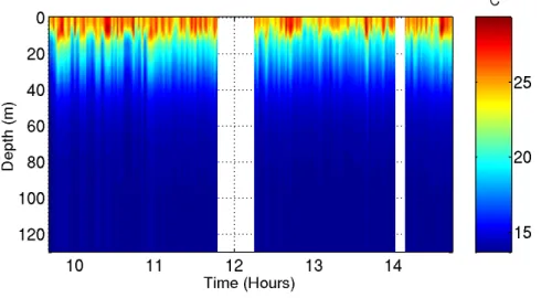
Figure 2 shows the reconstruction of the temperature profiles along time. Only profiles corresponding to successful source localization were taken into consideration and gaps in between were filled by linear interpolation in time. The gaps seen in the plot
Fig. 2 Reconstruction of the temperature profiles estimated. Only profiles corresponding to successful source localization are taken into consideration.
are due to the change of the emitted waveform. It is seen that significant difficulties are found in dealing with the strong thermocline. This is clearly the result of strong refraction that prevents the top receiver to receive a significant level of acoustic power. Although low precision was attained in estimating the first layer, it should be remarked that the source localization has filtered profiles with unlikely temperature estimates. The maximum estimated surface temperature is 28 ◦C for few time points, most of the time it is about 27 ◦C which is in agreement with the measurements.
4. CONCLUSIONS
MFT was applied to the MREA’03 sea trial using only receivers 1 through 3. The most important objective was to compare the proposed processors in application to real field data. The second objective was to verify whether source localization could serve as a validation tool for the environmental model estimates obtained through the MFT inver-sions. The first conclusion to be drawn is on the comparison of the global performance of the three processors. The performance was measured in terms of rate of successful source localization. The global performance was clearly superior for the MUSIC processor. In terms of validation of the environmental inversions using source localization, it can be said that the successful localization is not an unequivocal validation of the inversion result, but it clearly tends to give an idea on the overall quality of the inversion results contained in a run.
ACKNOWLEDGEMENTS
This work was financed by FCT, Portugal, under contract NUACE, POSI/CPS/47824/2002, and RADAR, POCTI/CTA/47719/2002.
REFERENCES
[1] J. Sellschopp and A. R. Robinson. Describing and forecasting ocean conditions during operation rapid response. In Proc. of the conf. on rapid environmental assessment, pages 35–42, Lerici, Italy, March 1997.
[2] C. Soares and S. M. Jesus. Broadband matched field processing: Coherent and inco-herent approaches. J. Acoust. Soc. Am., 113(5):2587–2598, May 2003.
[3] R. O. Schmidt. A signal subspace approach to multiple emmiter location and spectral estimation. Phd. dissertation, Stanford University, 1982.
[4] J. F. Boehme. Advances in Spectrum Analysis and Array Processing, volume 2, chap-ter 1, pages 1–63. Prentice-Hall, Engelwood Cliffs, 1991.
[5] C. Soares, S. M. Jesus, and E. Coelho. Acoustic oceanographic buoy testing during the maritime rapid environmental assessment 2003 sea trial. In D. Simons, editor, Proc. of European Conference on Underwater Acoustics 2004, pages 271–279, Delft, Netherlands, 2004.