Preliminary topology optimization of small unmanned aircraft wings for additive manufacturing

Engenharia

Preliminary Topology Optimization of Small

Unmanned Aircraft Wings for Additive

Manufacturing

Cátia Alexandra Louro Miguel

Dissertação para obtenção do Grau de Mestre em

Engenharia Aeronáutica

(ciclo de estudos integrado)

Orientador: Prof. Doutor Pedro Vieira Gamboa

“A person who never made a mistake never tried anything new.” Albert Einstein

Acknowledgements

I would like to thank all the people that accompanied me through this journey and made me a better person.

First, I would like to thank my supervisor Pedro Vieira Gamboa, for all the guidance, support and patience throughout this work. His motivation was essential for the accomplishment of the work.

Secondly to Pedro Alves and Pedro Carneiro for the advice and help through this work.

I would also thank my friends who, over these years, shared with me good moments and I will always keep with me. Thank you to André, António, Bruna, Cátia, Daniel, Flávia, Francisco, Gabriel, Inês, João Miguel, João Rocha, Luís Coelho, Luís Oliveira, Mara, Nicole, Nídia, Nuno, Pedro and Rodolfo.

Lastly, I would like to thank the most important people in my life, my parents. Without them, nothing would be possible, and I am grateful for all they have done for me. Thank you for all the love and courage you gave me!

Resumo

O Fabrico Aditivo (FA) descreve os processos que criam peças em 3D, sendo estas fabricadas camada-por-camada. A tecnologia do FA já abrange, hoje em dia, uma grande variedade de materiais, não havendo essa barreira quando é proposto um projeto. Permite também a produção de mais peças em menos tempo, o que faz com que haja uma redução de custos e de desperdício de material. A Otimização Topológica combina o método dos elementos finitos com fórmulas matemáticas de otimização, proporcionando assim uma melhor distribuição de material no domínio de referência da geometria em análise. Esta otimização pode ser aplicada de modo a melhorar o desempenho de produtos já existentes ou para criar novos. Ao juntar estas duas ferramentas, o FA com a otimização topológica, é possível criar estruturas mais leves, com maior rigidez e complexidade. O que antigamente não era fazível, devido à limitação nos moldes e ferramentas nos métodos tradicionais.

Esta dissertação procura a possibilidade de usar a otimização topológica como ferramenta para obter uma asa, para um avião não tripulado (UAV), mais leve. O objetivo é investigar as características de rigidez e resistência de uma asa, sendo apresentados diferentes casos para análise. O trabalho descreve os designs e os procedimentos numéricos, em que se enquadram a dinâmica dos fluidos computacional, as análises estruturais e a otimização topológica. A otimização foi realizada com o objetivo de minimizar a massa. Todo o procedimento numérico foi efetuado no software ANSYS.

Ao realizar este trabalho, houve um caso de estudo que se destacou apresentando uma redução de 74% da massa, ainda assim para os requerimentos da aeronave em questão são necessários mais estudos.

Palavras-chave

Abstract

Additive Manufacturing (AM) describes the processes which produce 3D parts, being these manufactured through a layer-by-layer procedure. The AM technology takes a wide variety of materials, so there is not a barrier in that field when a project is proposed. It also allows the part production in less time, reducing the costs and material waste. Topology Optimization combines the finite element method with mathematical optimization formulas, providing a better material distribution in the reference domain of the geometry under analysis. This optimization can be applied to improve the performance of existing products or to create new ones. By combining these two tools, AM and topology optimization, create lighter structures with greater rigidity and complexity is possible. Which previously was not possible due to the limitation in tools and molds of traditional methods.

This work searches the possibility of using topology optimization as a tool to obtain a lighter wing to an unmanned aerial vehicle (UAV). The objective is to investigate the stiffness and strength characteristics of a wing, being presented in different cases for analysis. This dissertation describes the designs and numerical procedures, in which are included computation fluid dynamics, structural analysis, and topology optimization. The optimization was realized with the aim of minimizing mass. The entire numerical procedure was performed in ANSYS software.

In this work, there is a study case which was evidencing, due to the 74% of weight reduction, but for the aircraft requirements in the study, more investigations are necessary, since the final design wing has, approximately, 1.5kg and the UAV should have a mass of 5kg.

Keywords

Content

2.1.3 Advantages and Disadvantages... 5

2.2 Materials ... 6

2.2.1 Polymers ... 7

2.2.1.1 Polylactic Acid (PLA) ... 7

2.3 Printing Cases of Unmanned Aerial Vehicles (UAVs) ... 9

2.3.1 FDM printed Fixed Wing UAV – AMRC UAV ... 10

2.3.2 RecordRotor ... 10

2.3.3 SULSA UAV ... 10

2.3.4 World’s First Jet-Powered, 3D-Printed UAV ... 11

2.3.5 EASYMAX 001 ... 11

2.3.6 University of Manito7gba – Team Kinect12 ... 12

2.3.7 Air Force Institute of Technology ... 13

2.4 Structural Optimization ... 15

2.4.1 Finite Element Method ... 15

2.4.2 Topology Optimization ... 16

2.4.3 SIMP: Solid Isotropic Material with Penalization ... 18

Chapter 3 ... 21

3.1 Software description ... 21 3.1.1 ANSYS ... 21 3.1.1.1 Workbench ... 21 3.1.1.2 Fluent ... 21 3.1.1.3 Mechanical ... 22 3.1.1.4 SpaceClaim/DesignModeler ... 22 3.1.2 CATIA ... 22 3.1.3 XFLR5 ... 22 3.2 Numerical Setup ... 22 3.2.1 Analysis setup ... 23 3.2.2 Fluent ... 23 3.2.2.1 Mesh ... 24 3.2.2.2 Setup ... 26 3.2.3 Mechanical ... 27 3.2.3.1 Engineering Data ... 28 3.2.3.2 Static Analysis ... 28

3.2.3.2.1 Stress and strain formulas for an isotropic material ... 28

3.2.3.2.2 Stress and strain formulas for an orthotropic material ... 29

3.2.3.2.3 Setup ... 30 3.2.4 Topological Optimization ... 31 3.2.4.1 Analysis Settings ... 31 3.2.4.2 Optimization Region ... 32 3.2.4.3 Response Constraints ... 32 3.2.4.4 Objective ... 32 Chapter 4 ... 35

4.2.1 Mesh Element Quality ... 37

4.2.2 Results ... 38

4.2.2.1 Equivalent Stress ... 39

4.2.2.2 Total Deformation ... 40

4.2.2.3 Percentage of Stress Error ... 41

4.3 Topology Optimization ... 41

4.3.1 Optimization Region ... 41

4.3.2 Results ... 42

4.4 Post-processing and design verification ... 45

4.4.1 Final design ... 46

4.4.2 Structural Analysis ... 47

Chapter 5 ... 49

Conclusions and Future Work ... 49

5.1 Conclusions ... 49 5.2 Challenges ... 49 5.3 Future Work ... 50 Bibliography ... 51 Appendixes ... 55 Appendix A ... 55 Appendix B ... 56 Appendix C ... 58 C.1 – First Case ... 58 C.2 – Second Case ... 58 C.3 – Third Case ... 59 Appendix D ... 60

List of Figures

Figure 1.1 – Generic process of CAD to part. ... 1

Figure 2.1 – Schematic of fused deposition molding (FDM) process. ... 4

Figure 2.2 – SULSA. ... 10

Figure 2.3 – Aurora Flight Sciences’ high-speed UAV is 80 percent 3D-printed with Stratasys’ additive manufacturing solutions. ... 11

Figure 2.4 – EASYMAX 001. ... 11

Figure 2.5 – View of one half of the wing assembly. ... 12

Figure 2.6 – Carbon-fibre veneer adhered to frame module, making up the wing surface. .... 12

Figure 2.7 – Final geometry that was printed. ... 13

Figure 2.8 – Initial design space for TO, where blue corresponds to design space and red and pink corresponds to non-design space, presented at left. Topology optimized is illustrated at right. ... 13

Figure 2.9 – 3D printed wing. ... 14

Figure 2.10 – Timeline representing development of AM processes and UAV fabrications using AM. ... 14

Figure 2.11 – Three different structural optimization types. a) Size; b) Shape; c) Topology. . 15

Figure 2.12 – Example of a topological optimization. ... 16

Figure 2.13 - SIMP flow chart. ... 18

Figure 3.1 – Introduction to the overall procedure. ... 23

Figure 3.2 – ANSYS Workbench. ... 23

Figure 3.3 – Mesh around the aerofoil. ... 24

Figure 3.4 – Representation of element quality in ANSYS Fluent. ... 25

Figure 3.5a) – Domain boundaries definition, focus in symmetry and outlet. ... 25

Figure 3.5b) – Domain boundaries definition, focus in symmetry and inlet. ... 25

Figure 3.6 – Axis system illustration. ... 27

Figure 3.7 – Representation of the effect of the density filter on an arbitrary design variable distribution... 33

Figure 3.8 – Influence of filter factor b on the optimal layout. The ground structure consists of 120x40=4800 4-node elements and the volume is restricted to 50% of the design domain. ... 34

Figure 4.1 – Image of the aerofoil obtained in XFLR5. ... 35

Figure 4.2 – Illustration of the wing root. ... 36

Figure 4.3 – Illustration of the wing root. ... 36

Figure 4.4 – Illustration of the wing root. ... 37

Figure 4.6 – Representation of the element quality, for the first case. ... 37

Figure 4.7 – 10-noded tetrahedron element. ... 38

Figure 4.8 – Distribution of equivalent (von-Mises) stress over the wing, in Pa, where: a) first case, b) second case and c) third case. ... 39

Figure 4.9 – Distribution of deformation over the wing, in m, where: a) first case, b) second case and c) third case. ... 40

Figure 4.10 – Percentage of stress error, where: a) first case, b) second case and c) third case. ... 41

Figure 4.11 – Representation of exclusion and design regions, for the first case. ... 42

Figure 4.12 – Representation of exclusion and design regions, for the second case. ... 42

Figure 4.13 – Representation of exclusion and design regions, for the third case. ... 42

Figure 4.14 – Representation of the removed material, of the first case. ... 43

Figure 4.15 – Representation of the retained region, of the first case. ... 43

Figure 4.16 – Representation of the removed material, of the second case. ... 43

Figure 4.17 – Representation of the retained region, where the tip of the wing is detached, of the second case. ... 43

Figure 4.18 – Representation of the removed material, of the third case. ... 44

Figure 4.19 – Representation of the retained material, of the third case. The image focus on wing’ tip to the interior. ... 44

Figure 4.20 – Representation of the final geometry, as viewed from the side, in CATIA. ... 46

Figure 4.21 – Representation of the optimized geometry, from the top, in CATIA. ... 46

Figure 4.22 – Representation of the support from the connection between wing-fuselage. ... 47

Figure C.5 – Objective convergence vs objective convergence criterion. ... 59 Figure D.1 – Dimensions from the support geometry of the connection between wing-fuselage. ... 60

List of Tables

Table 2.1 – Material properties of bulk PLA. ... 7

Table 2.2 – Ultimate tensile strength (MPa) of different thermoplastics 3D-printed by FDM. ... 8

Table 2.3 – Classification of UAVs as defined by UVS International. ... 9

Table 2.4 – Name of UAVs or printed parts for each type of AM technique. ... 9

Table 2.5 – Methods used for large ISE or IS topologies in generalized shape optimization. ... 17

Table 3.1 – Orthogonal Quality mesh metrics spectrum. ... 24

Table 3.2 – Correspondence of percent of the number of elements with the classification of orthogonal quality, a mesh metric from ANSYS Fluent. ... 25

Table 3.3 – Properties of unidirectional carbon fibre reinforced plastics and PLA. ... 28

Table 3.4 – Values of C for each type of element. ... 30

Table 4.1 – Aircraft’s data on Air Cargo Challenge 2017. ... 35

Table 4.2 – Results from the mesh analysis used on different geometries. ... 38

Table 4.3 – Results from Mechanical analysis. ... 39

Table 4.4 – Results of the Topology Optimization, to the different study cases. ... 42

Table 4.5 – Results of the final design, obtained in ANSYS. ... 47

Table A.1 – Results from XFLR5, to a fixed speed of 24 m/s. ... 55

Nomenclature

b Filter factor [-]

B Bulk modulus [Pa]

C Constant [-]

C1ε Constant [-]

C2ε Constant [-]

Cµ Constant [-]

CL Lift coefficient [-]

Cm Constitutive matrix [Pa]

E Elastic Modulus [Pa]

E0 Elastic matrix of initial solid element [Pa]

Ei Elastic matrix [Pa]

F External force vector [N]

G Shear Modulus [Pa]

h Volume ratio [-]

H Sensitivity filter [-]

k Turbulent kinetic energy [m2_/s2_]

K Global stiffness matrix [Pa]

L Lift [N]

Lal Adjoint load vector [N]

N Total number of discrete numbers [-]

p Penalization [-]

rfilter Mesh filter radius [m]

S Wing area [m2_]

Sut Ultimate tensile strength [Pa]

u Displacement vector [m]

U Global displacement vector [m]

X Design variable vector [-]

𝑣

̅

V Velocity [m/s]

V0 Initial volume [m3]

Vad Adjoint displacement vector [m]

wj Weight function [kg]

xi Position of element i [m]

xj Position of element j [m]

xt Ultimate longitudinal tensile strength [MPa]

Greek symbols

ε Strain [-]

εd Dissipation rate [m2/s2]

σ Stress [Pa]

σε

Constant (Turbulent Prandtl number for dissipation

rate) [-]

σk

Constant (Turbulent Prandtl number for kinetic

energy) [-]

σy Yield Strength [Pa]

σlim Yield stress limit [Pa]

σvm Von Mises stress [Pa]

ρ Density [kg/m3_]

ρi Element i density [kg/m3]

𝜌̃ 𝑖 Filtered i density [kg/m3]

ρj Element j density [kg/m3]

ρmin Minimum limit of element relative density [kg/m3]

µ Dynamic Viscosity [kg/(m.s)]

𝑣 Poisson’s ration [-]

Acronyms

3D Three Dimensional

ABS Acrylonitrile Butadiene Styrene AM Additive Manufacturing

ANSYS Analysis of Systems

BC Boundary Condition

CAD Computer-Aided Design

FDM Fused Deposition Modelling FEA Finite Element Analysis FEM Finite Element Method FGM Functionally Graded Materials

PLA Polylactic Acid

SIMP Solid Isotropic Material with Penalization

TO Topology Optimization

UAV Unmanned Aerial Vehicle UBI Universidade da Beira Interior

Chapter 1

Introduction

1.1 Motivation

Nowadays, parts are possible to manufacture through Additive Manufacturing (AM) technology, more specifically 3D printing, which consists of a print of a three-dimensional model generated using a CAD system, created by successive layers of material [1]. The original name for 3D printing was rapid prototyping because a product could be rapidly and automatically created without any complexity [2]. The term AM was given by the committee (F42) of American Society for Testing and Materials (ASTM), in 2009 [2]. Since then, multiple new technologies using different materials, including metallic, ceramic and polymeric materials, became commercially available [3]. AM technology has been studied due to its advantages because it can be used to remove or simplify many of multi-stage processes, reducing time when compared to traditional methods. AM process is illustrated in Figure 1.1.

Figure 1.1 – Generic process of CAD to part [4].

AM can be combined with Topology Optimization (TO), which is a numerical method that enables the weight optimization of any geometry complying with previously requirements.

These new methods and technologies allow the reduction of using parts that leads to fewer critical failures. Considering these implications, safer aircrafts could be produced, and many lives could be saved. Thus, the need to continue the development of these tools is crucial.

1.2 Objectives

The purpose of this dissertation is to investigate the possibility of using TO in the design of a small unmanned aerial vehicle (UAV) wing that is to be produced by an additive manufacturing technology. For that, the following tasks were defined:

• Design geometry in CATIA V5 for implementation on CFD analysis;

• Structural analysis in ANSYS for different design geometries, applying the boundaries conditions and the results from CFD analysis;

• Topology optimization of previous designs, with the intention of weight reduction.

1.3 Dissertation Outline

This dissertation is divided into 5 chapters. The first and current chapter includes motivation and objectives.

The second chapter is dedicated to the literature review, where the technologies of AM are presented, as well as, the advantages and disadvantages, including the materials used. Some printing cases of UAVs and parts of its are also presented. TO is presented at the end of this chapter, emphasizing the Solid Isotropic Material with Penalization (SIMP) method, where the formulas behind the method are shown.

The numerical methods are described in the third chapter. Firstly, the software used is described. Then, the numerical setup is presented, where it is divided into 4 sub-sections. The first sub-section is a brief presentation of ANSYS Workbench. The second is dedicated to Fluent, where the used model, mesh and boundary conditions (BCs) are being described. The third includes the mechanical study, where the material’s properties are presented, and an explanation of the setup. The fourth is dedicated to topology optimization.

The fourth chapter refers to the study cases and the results from mechanical and topology optimization.

Chapter 2

Literature Review

2.1 Additive Manufacturing

2.1.1 Definition

In 2012, ASTM defined AM technology as capable of “joining materials to make objects from 3D model data” [1]. The initial purpose of the technology was to create prototypes, for all sectors, in a flexible and fast manner [2].

AM involves processes based on continuous deposition of material, layer-by-layer until a physical object is created without labor resources, following instructions from a computer with a virtual model designed in a CAD system. In these processes, metal, polymers, or ceramics materials are used, through highly specialized machines [2]. For each of these technologies, there are at least two materials: the production material and the support material. The support is, in most of the cases, cleaned and becomes a manufacturing residue [5]. With the evolution of materials and processes, AM became a natural tool to solve some specific problems for small series direct production (rapid manufacturing), tooling production and more recently a powerful tool to produce cost-effectively complex parts. Nowadays, faster and cheaper AM techniques have been developed with high print quality. Polymer materials for 3D printing are being produced with a wider range of properties [6].

These technologies are revolutionizing the world of manufacturing, bringing forward the so-called Fourth Industrial Revolution (4.0 Industry), where the production processes tend to become increasingly efficient, autonomous and customizable [3].

2.1.2 Processes

The commercial AM most used are:

1. Stereolithography (SLA)

The basic concept of stereolithography is photocurable resin printing, typically acrylic or epoxy, by exposing it to ultraviolet (UV) light of a specific wavelength, and then the exposed 2D-patterned resin layers become solid through a process called photopolymerization [1, 2, 6].

2. Fused Deposition Modelling (FDM)

It is one of the most used techniques which uses a spool of a thermoplastic filament with varying diameters to be melted and extruded through a heated nozzle. The materials used are nylon, Acrylonitrile Butadiene Styrene (ABS), Polylactic Acid (PLA) and aerospace grade UltemTM_{. This}

technique is based on automatic deposition of filament material and a filament of support one. T5his process is repeated layer-by-layer, until the physical model is finished, as illustrated in Figure 2.1. In the end, the support material is taken out through a process like ultra-sound bath. Recently, thermoplastics with higher melting temperatures such as PEEK can already be used as materials for desktop 3D printing, which are the most popular consumer-level polymer composites 3D printers.

As long as the errors are below the accuracy level of the machine process (≈ 0.5mm), they are acceptable. The machine’s language is STL and then it prints one layer (2D) on top of the other, forming at the end a 3D object [2, 6, 7, 8].

4. Multi Jet Modelling (MJM) or Polyjet

It is a process where a print head containing hundreds of nozzles selectively spreads in a surface a photopolymeric material that is cured by the incidence of a specific wavelength. Another print head spreads support material, normally in form of a gel that is also polymerized. It is a continuous process where the platform is reduced to a tenth of a millimetre for each layer. In the end, the support material is removed through a water jet [2].

5. 3D Printing (3DP)

It was developed by the Massachusetts Institute of Technology (MIT) and, today is one of the most popular because of the low costs of acquisition and operation. It is a type similar to SLS where a multi-nozzle print head selectively spreads a liquid binder in a platform with a powder. The binder reacts with the powder to compose a layer while the platform is moved down. The process repeats until the end of the part. The quality of the final product depends on powder particle size, the viscosity of the binder, binder-powder interaction, and the speed of the binder deposition [2, 6].

2.1.3 Advantages and Disadvantages

• Energy optimization: According to the USA Energy Department, AM can reduce energy costs by 50% and material costs by 90%. The design and fabrication processes have been reduced from weeks to a few hours [2, 6].

• Reduction in material waste: It is supposed that with AM, the only material required is the one used to create parts. However, it is not completely true because sacrifice support structures sometimes are necessary and some materials, special polymers, degrades with continuous use under heating [2].

• Special tooling and speed: There is great flexibility to produce many different parts at the same time, without the necessity of special tooling or equipment. AM systems are capable to manufacture 3D components and products directly from raw materials and 3D design data [1, 2].

• Design optimization: It is possible to produce complex shapes, so our mind is the limitation [1, 6].

• Possibility to create low quantities of products, or just one, providing the absence of cost relating to tools, as well as, reducing the number of parts in inventory since could be produced on-site [1].

• Producing parts neglecting the prototype development phase. A direct translation of design to component [3, 7].

Disadvantages:

• Slow process speed [1].

• Poor dimensional accuracy compared to some conventional processes [1]. • Rough surface finish and problems with process repeatability [1].

• The inherent anisotropic property of the printed parts. A result of AM techniques is that the microstructure of the materials would tend to grow in a certain direction causing different mechanical property along the layer. Consequently, parts manufactured through additive processes show a preferential bearing direction, normally the one along which the material is deposited [8, 9].

• AM is more economical when total build volume is lesser than 130 units, below that injection moulding should be used. Additional processes are needed to make the material into the forms that are suitable for AM processes, that is why material costs are higher than conventional techniques [8].

2.2 Materials

The materials types used in AM processes have a large range, including metallic, ceramic and polymeric materials along with combinations in the form of composites, hybrid or functionally graded materials (FGM) [3]. Each process (mentioned in 2.1.2) requires different materials [8]. Mechanical properties of AM parts can be affected by unprinted materials and the technique used. Nowadays, there are no standard tests for mechanical characterization because of the undefined mechanical behaviour of 3D printed parts, and this happens for two reasons. Firstly, because of the high number of parameters to control during the process. Secondly because of the high anisotropy, which is defined by their manufacturing history, as the resistance of the raw material and the cohesive forces between bonded layers [6]. Dizon et al. (2017) [6] concluded that 3D-printed materials have large anisotropy, especially for the FDM and SLS printed parts. The AM aim is to print a part with excellent quality with minimal anisotropy.

Between these materials, polymers have been mostly used perhaps due to their widespread use in the first-generation rapid prototyping machines [3]. Polymers have relatively lower melting and glass transition temperatures, which make it easier to flow at a relatively lower temperature than ceramics and metals. Bonding involving metals and ceramics are not easy to

required strength, and then they reinforced the parts with carbon fibre rods and polyester films for better strength.

Relatively to the characterization of powder materials and final products, Caputo et al. [11] made a study. Since the processes of AM involve heat exchange phenomena, must be taken into account the knowledge of the thermal behaviour of starting powder materials. Another important aspect is their density and porosity. Porosity is a property that strongly affects the quality of parts and for the measure of this feature there are ultrasonic non-destructive testing, Archimedes method or micro X-ray computed tomography. Advanced image processing techniques are useful in the AM environment to develop better quality control and reliability. Non-destructive characterization methodologies allow to detect failures and to describe the structure. They concluded that measuring the properties of powders is mandatory for the industry to select proper raw materials.

2.2.1 Polymers

Polymers are macromolecules formed through smaller structural unities. They have structures much more complex than metals or ceramics parts and they can be easily processed. Nevertheless, they have low relative strength, elasticity module and operating temperature limits.

Polymers are subdivided into two classes: thermoplastics and thermosetting. A thermoset is a material that cures into a given shape, generally through the application of heat (curing is an irreversible chemical reaction in which permanent connections are made between the material’s molecular chains). A thermoplastic is a polymer that shapes with the application of heat,i.e. its viscosity becomes smaller on heating. Cooling to room temperature makes the strongest thermoplastics [10].

2.2.1.1 Polylactic Acid (PLA)

The most frequent source materials for commercially-available FDM printers are ABS and PLA. Bulk PLA characteristics can be seen in Table 2.1.

Table 2.1 – Material properties of bulk PLA [12].

Material property Units Value

Density (ρ) kg/m3 ₁₂₄₀

Elastic modulus (E) Pa 3500×106

Shear modulus (G) Pa 1287×106

Poisson’s ratio (v) - 0.36

Yield strength (σy) Pa 70×106

Ultimate tensile strength (Sut) Pa 73×106

Industrial and general use of PLA is increasing due to the fact of its biocompatibility with the environment, and for this reason, now many desktop consumer printer models use, exclusively, PLA.

Torres et al. (2015) [12] present a study where they tested torsion of PLA materials resulting from FDM and the effects of processing parameters including layer thickness, percent infill, and post-processing via heat treatment. They concluded that heat treatment can cause an increase in strength, especially in low-infill components. But this increase in strength provides a loss in ductility.

Some studies have recently reported the tensile strength of different polymers, as summarized in Table 2.2.

Table 2.2 – Ultimate tensile strength (MPa) of different thermoplastics 3D-printed by FDM [13].

Raster Angle ABS Polypropylene Polycarbonate PLA PEI

90º 26 32 19 54 40

0º 34 36 59.7 58 59

Authors Rezayat et al. Carneiro et al. Hill et at. Letcher et al. Bagsik et al.

These studies revealed that PLA has a better mechanical response than the other thermoplastics polymers, and in tensile strength plane these materials are anisotropic, with the strength along the direction of extrusion (0º) exceeding that in the transverse direction (90º). Research by Ahn et al. [13] showed that the printing orientation and air gap had the most significant impact on the mechanical properties of the printed objects; but on the other side, the printing orientation and the platform temperature have a significant impact on structural inhomogeneity.

Y. Song et al. (2017) [13] quantify anisotropy and asymmetry of the mechanical response of PLA parts produced by FDM. The elastic material response was transversely isotropic for 3D-printed specimens and isotropic for injection-moulded specimens. They study specimens of porosity of order 1% and conclude that the porosity of 3D-printed material can be minimised by optimising the temperature and speed of extrusion, as well as, the speed of the printing head. Manufacturing by 3D-printing increases the crystallinity of the material, reducing its ductility and increasing the fracture toughness. The elastic response of 3D-printed material is

as a function of strain, indicating the presence of damage mechanisms in conjunction with material’s plasticity.

2.3 Printing Cases of Unmanned Aerial Vehicles (UAVs)

Unmanned aerial vehicles are gaining popularity due to their application in military, private and public sector, especially where human operator is not required. Evolution of UAVs started during World War II and it has come a long way for all operations, military and non-military. Birds and insects are the inspiration for some UAV’s designs and the most desired are the light-weight UAVs due to a better performance in terms of shorter take-off range and longer flight endurance. When operating at low Reynolds number the performance largely depends upon a complex combination of specific and precisely orientated geometrical forms, for example, flapping wing UAV has several potential benefits over fixed wings, as a better manoeuvring, low speed, landing, and vertical take-off. Although a UAV design is specific to its mission requirements, having high endurance is something that all have in common [8]. Table 2.3 summarizes the classification of UAVs as defined by UVS International.

Table 2.3 – Classification of UAVs as defined by UVS International [8].

UAV category Range [km] Flight altitude _[m] Endurance [hours] Max. take-off _{weight [kg]}

Micro <10 250 1 <5

Mini <10 150-300 <2 <30

Medium range 70-200 5000 6-10 1250

Medium altitude long

endurance >500 14000 24-48 1500

High altitude long endurance

>2000 20000 24-48 12000

Recent research on cellular structures and topology optimization have resulted in complex light-weight UAV structures that cannot be fabricated using conventional manufacturing techniques, so AM presents itself as a better option because there is no design limit [8]. Table 2.4 shows which AM technology was used for a UAV component or even an entire UAV.

Table 2.4 – Name of UAVs or printed parts for each type of AM technique [8]. Types of AM techniques Name of UAVs/ printed parts

FDM Fully printed; AMRC UAV; VAST

UAV; Frame, gear, tail

Polyjet Lattice structure; Wing strut;

Ornithopter; Replica of insect wing

SLA Entomopter; Stingray UAV;

Flap; Wind tunnel; UAV model

SLS SULSA UAV; Scaled-down UAV;

2.3.1 FDM printed Fixed Wing UAV – AMRC UAV

During the built process of FDM is necessary a broad number of support material in order to prevent deformation, and this adds a direct material cost and significantly increases built time. In 2014, a prototype UAV was design, manufacture and flight test by a team of engineers from AMRC’s (Advanced Manufacturing Research Centre) new Design & Prototyping Group (DPG), entirely of ABS plastic (ABS-M30), using FDM technology. For printing large components, such the airframe, FDM was chosen, took less than 24 hours, which would be unthinkable because before of AM optimization, the airframe would take 120 hours to produce. The UAV showed good stability, and low aerodynamic noise at speed indicated an efficient wing design [14].

2.3.2 RecordRotor

In 2015, Altair Engineering in cooperation with Politecnico di Torino developed components for a structure of a multi-rotor, named RecordRotor. The challenge was to interface arms, consisting of carbon fibre tubes, with motor or frame, in 7075 Alloy. They use topology optimization to minimize the weight and additive manufactured polymer components played an important role in the prototype which was designed at the upper boundary of the normative with an MTOW of 25kg. They demonstrate that with a scientific methodology and with the support of innovative design tools was possible to construct high-performance components for the aerospace industry, with optimization included [7].

project were that they needed the use of a launch catapult and a belly landing because there was no undercarriage to keep complexity and weight down [15, 16].

2.3.4 World’s First Jet-Powered, 3D-Printed UAV

Aurora Flight Science and Stratasys Ltd developed a 3D-printed, jet-powered UAV with the ability to reach speeds up to 241 km/h. It has a wingspan of 3m and weighs only 15kg, as illustrated in Figure 2.3. 80% of the UAV was created using FDM process and the fuselage was made of nylon and the engine exhaust duct was 3D-printed in metal [17].

Figure 2.3 – Aurora Flight Sciences’ high-speed UAV is 80 percent 3D-printed with Stratasys’ additive manufacturing solutions [17].

2.3.5 EASYMAX 001

EASYMAX 001 has a wingspan of 1527mm, as presented in Figure 2.4. It is easily printed and possible to buy it, with a cost of 20$ and with an instruction manual included. Even the wing and the fuselage have a 3D structure reinforcement, which makes the UAV very rigid while maintaining a lightweight, even when it is made only from polymers [18].

2.3.6 University of Manito7gba – Team Kinect12

In 2011, the Composites Innovation Centre (CIC) requested Team Kinect12, from the University of Manitoba, to develop a manufacturing process for a small airplane wing, which utilizes rapid prototyping. The objectives that the client established was that the wing should weight no more than 0.45kg and must structurally be capable of lift and support a 2.3kg UAV. The process should also avoid the traditional methods of UAV wing construction and should be applicable to other structures.

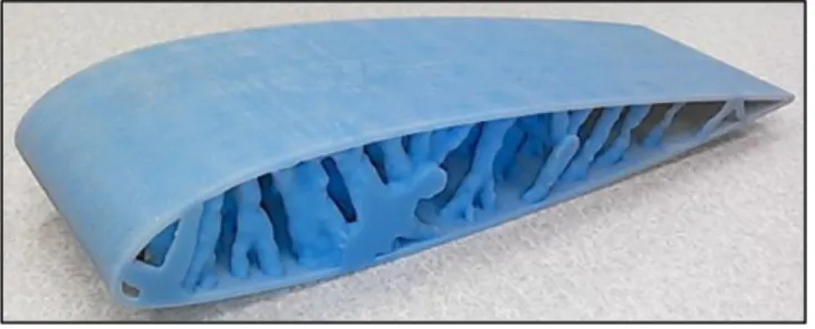
The final wing design, of Team Kinect12, consists of RP frame modules, carbon fibre veneers, webs, and a spar. The veneers are adhered to the exterior shell to provide torsional strength for the wing and additionally provide the surface of the aerofoil, as represented in Figure 2.5 and Figure 2.6. The spar is to provide high specific strength and covers the entire span of the wing at 25% of the chord. The frame is produced in nine different modules, printed in ABS [19]. Figure 2.7 illustrates the final geometry that was printed through rapid prototyping.

Figure 2.7 – Final geometry that was printed [19].

The team’s setback was that RP machine had a lower resolution than some of the details provided in CAD models, so these details were not printed, and thus were not included in final geometry. But still, they were able to accomplish all the requirements established by CIC.

2.3.7 Air Force Institute of Technology

Walker et al. (2015) [20] decided to join AM with TO with the objective of creating a complex wing structure. The TO objective was minimizing compliance, which means maximizing the stiffness. They decided to apply the optimized wing in a UAV due to the relaxed airworthiness requirements. The final objective of their work was focused only on the main wing body structure, disregarding internal components like fuel tank, electronics, and cables. The wing structure had two small structural constraints near the centre of the design space. All the analysis was conducted considering only the skin of the wing, spars, and ribs. The wing was structurally constrained at the wing root and aerodynamic forces were applied for defined conditions.

For TO, the wing skin was considered a non-design space. The design space, the region where the optimization occurred, was the wing interior. And in the centre of design space, there were two small structural constraints, which belongs to non-design space (the region where optimization does not occur). The optimization constraint used was to maintain a volume fraction of the overall design space of less than 30 percent and the material used by them was an aluminum alloy. Figure 2.8 shows the initial design after the optimization and shows the structure after TO.

repres ent ing d ev elo pm ent o f A M pro ces ses a nd U A V fa bri ca ti on s us ing A M [8 ].

Figure 2.9 presented the 3D printed wing, which was the purpose of the work.

Figure 2.9 – 3D printed wing [20].

Figure 2.10 is representing the timeline of the evolution of AM’s processes and development of UAVs.

2.4 Structural Optimization

A continuum structure, relatively to the structural optimization, can be divided into Shape Optimization, Size Optimization and TO, as illustrated in Figure 2.11. Compared to the first two optimizations, TO can change the structure of the part, achieving designs that are not greatly constrained by the nature of the initial design [21, 22]. TO matches Finite Element Method (FEM) with mathematical formulas of optimization, with the aim of providing the best material distribution [23].

Figure 2.11 – Three different structural optimization types. a) Size; b) Shape; c) Topology [24].

2.4.1 Finite Element Method

The FEM is a mathematical approach in which to solve a problem it subdivides into smaller elements that keep the same properties compared to the initial. Differential equations are used to describe these elements and are solved by mathematical models to obtain results with more accuracy, but only gives an approximate solution [25, 26]. Several Finite Element (FE) based methods have been developed for topology optimization of continuum structures. The Finite Element Analysis (FEA) method, originally introduced by Turner et al. (1956) [27], is a powerful computational technique for approximate solutions to a variety engineering problems, having complex domains subjected to general BCs. It has become an essential step in the design or modelling of a physical phenomenon. This physical phenomenon occurs in a continuum domain involving several variables and the field of variables vary from element point to point, possessing an infinite number of solutions in the domain. FEA reduces the problem to a finite number dividing the domain into elements and expressing the unknown field variable in terms of the assumed approximating functions within each element. These functions are defined by the nodes, and these nodes are usually located along the element boundaries, and they connect adjacent elements [28, 29].

2.4.2 Topology Optimization

The coupling between AM and TO provides innovations forms, which with traditional manufacturing could be impossible to turn them into a part, but with additive manufacturing it is conceivable, and it can be applied in plastics, metals, etc. [5]. Over the last decade, TO has appeared as one of the numerous optimization techniques being used by most aircraft manufacturers due to its capability to generate light-weight conceptual designs [30]. The purpose of this optimization is to find the optimal layout within a specified region, knowing the support conditions, the applied loads and the volume constraints, being unknown the shape, the physical size and the connectivity of the structure [31]. TO has important practical applications by the manufacturing (i.e. car and aerospace) industries and has a significant role in micro and nanotechnologies [28].

In 1977, Prager and Rozvany [28] formulated the first general theory of topology optimization. Many optimization methods such as homogenization technique (Bendsøe and Kikuchi 1988 [28]), solid isotropic material with penalization (SIMP) (Bendsøe 1989; Zhou and Rozvany 1991 [28]) and evolutionary structural optimization (ESO) (Xie and Steven 1993, 1997 [28]) have been developed. SIMP, that was developed in the late eighties, and BESO is the most widely used algorithms, owing to their efficiency and simplicity [22, 32]. BESO (bi-directional ESO) is the latest version of ESO. It is a combination of additive evolutionary structural optimization (AESO) and ESO. In this method, the wasteful material is removed while efficient material is added to the structure, at the same time. However, BESO is limited to the TO of an objective function such as mean compliance with a single constraint, as structural volume [28, 29, 33]. SIMP will be discussed later in subchapter 2.4.3 since will be the method used in this dissertation. As previously presented AM materials are constituted by production material and the support one and this optimization can match both, as exemplified in Figure 2.12.

TO problem can be defined as the search for the best allocation or distribution of material in a given design space. The reference domain Ω (Ω Є R3_{) is determined by the design space, loads} and BCs. The design space corresponds to the interior of the objects and a non-design space corresponds to the skin of the object [5].

About existing topological optimization models, these can be divided according to the type of topology involved. Taking in consideration that the first term corresponds to the base material and the second to the type of elements, there are four large groups being designated as Solid (IS), Solid/Empty (ISE), Anisotropic-Solid/Empty (ASE) and Solid/Empty/Porous (ISEP) (includes Solid/Empty/Composite (ISEC) and Isotropic-Solid/Empty/Composite-Porous (ISECP)) [30]. For simplicity, the ISE and IS topologies are specified in this work. Within the models ISE and IS there are used the following strategies: Solid Isotropic Microstructures with Penalization (SIMP), Optimal Microstructures with Penalization (OMP), NonOptimal Microstructures (NOM) and Dual Discrete Programming (DDP). Below explained the strategies in Table 2.5:

Table 2.5 – Methods used for large ISE or IS topologies in generalized shape optimization [32].

SIMP as becoming generally accepted in topology optimization as a technique of considerable advantages.

SIMP OMP NOM DDP

Microstructure of elements

Solid, isotropic Optimal

nonhomogeneous Nonoptimal nonhomogeneous Solid, isotropic Additional penalization

Yes Yes No Not necessary

Homogenization necessary No Yes Yes No Number of free parameters 1 2D:3ou 4 3D:5 ou 6 >1 1

Available for: All combinations

of design

constraints

Compliance All combinations

of design constraints Compliance Penalization adequate Yes Yes No -

2.4.3 SIMP: Solid Isotropic Material with Penalization

Figure 2.13 - SIMP flow chart [22].

The term “SIMP” is sometimes called “material interpolation”, “power law”, “artificial material” or “density” method [28]. The basic idea of this method is discretizing the design domain by finite element mesh and optimize the density variables associated to each element within the discretization, as represented in Figure 2.13 [33]. The design variables are a series

degree of penalization [30]. The relationship of elastic matrix Ei, the effective Young’s modulus, and element density ρi in optimization process can be written as

𝐸𝑖= 𝜌𝑖 𝑝

𝐸0 (2.1)

where p is a penalization value and E0 elastic matrix of the initial solid element [34]. For p=1,

the problem corresponds to the classical ‘variable thickness sheet optimization’ which is studied by Cheng and Olhoff and lots of grey density elements 0<ρi<1 which have no physical

meaning are obtained. Choosing p too low or too high either causes too much grey scales or too fast convergence to local minima, and lots of numerical examples show that p=3 ensures good convergence to almost 0-1 solutions [33].

SIMP is used in practice for highly complex non-convex problems and most commercial TO software have implemented SIMP for TO, being ANSYS one of them [22, 28].

Chapter 3

Numerical Methods

3.1 Software description

Nowadays, technology allows the numerical study without experimental tests, giving the opportunity to realize studies that in an experimental way have a high cost. In this chapter, it will be discussed the software used, in a succinct way.

3.1.1 ANSYS

ANSYS is the original name for commercial products. The company develops a complete range of CAE (Computer Aided Engineering) products. It is a general-purpose finite-element modelling package for numerically solving a wide variety of mechanical problems. These problems include static/dynamic, structural analysis (both linear and nonlinear), heat transfer, and fluid problems, as well as acoustic and electromagnetic problems [35].

3.1.1.1 Workbench

ANSYS Workbench helps drive all of the simulations in a single environment. The platform guides the user through complex multiphysics analyses with drag and drops simplicity, providing bi-directional CAD connectivity [36]. ANSYS Workbench is often used in conjunction with CAD software such as DesignModeler or SpaceClaim.

3.1.1.2 Fluent

ANSYS Fluent provides comprehensive modelling capabilities for a wide range of incompressible and compressible, laminar and turbulent fluid flow problems. Steady-state and transient problems can be performed. In this type of analyse a broad range of mathematical models for transport phenomena is combined with the ability to model complex geometries. A very useful group of models in Fluent is the set of free surface and multiphase flow models, therefore, can be used for analysis of gas-liquid, gas-solid, liquid-solid and gas-liquid-solid flows. Accurate and robust models are a vital component of Fluent suite of models [37].

3.1.1.3 Mechanical

Mechanical is a module in ANSYS to set up and run structural analyses. Topology optimization was introduced in 2018 with ANSYS 18.0, integrating its own solver and pre and post-processing tools [24].

3.1.1.4 SpaceClaim/DesignModeler

SpaceClaim and DesignModeler are CAD software integrated into several modules of ANSYS. SpaceClaim is the most recent and more upset to topology optimization because it can read STL files exported from Mechanical and post-process the geometry before design validation. The geometry is converted then into a solid for ANSYS Mechanical to analyse again as validation process.

3.1.2 CATIA

It is a multi-platform software suite for CAD, computer-aided manufacturing (CAM), CAE developed by the French company Dassault Systèmes.

3.1.3 XFLR5

XFLR5 is an analysis tool for aerofoils, wings, and planes operating at low Reynolds Numbers.

3.2 Numerical Setup

In this chapter, the numerical methods and the numerical setup will be presented. Firstly, ANSYS Workbench will be explained. The second section is dedicated to ANSYS Fluent, describing the flow properties, that uses various convergence schemes to equate the flow properties along the boundaries and the principal aim of this section is to calculate lift, drag and pressure distribution along the wing. In this section mesh quality and model, setup is described. The third section corresponds to the Mechanical part and material data is provided, the mesh quality and the steps that have been taken in setup, in a general way, because there is be given more emphasis of this part in the next chapter. The fourth section refers to the

Figure 3.1 – Introduction to the overall procedure.

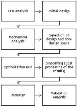
3.2.1 Analysis setup

Figure 3.2 shows a typical setup in ANSYS Workbench. Firstly, an analysis is made in Fluent, in order to determine the wing’s pressure distribution. Then, after the meshing is done in Static Structural and the loads are applied, the topology optimization can be initiated with the results from the two-previous analysis. The last analysis in Mechanical is to validate the design.

Figure 3.2 – ANSYS Workbench.

3.2.2 Fluent

Wing structures have a significant role because they are responsible to create lift. In movement, pressure distribution around the aerodynamic surface is created, which translates into the aerodynamic force. Fluent is used to determine the pressure distribution around the wing surface, in this dissertation.

3.2.2.1 Mesh

Figure 3.3 – Mesh around the aerofoil.

Figure 3.3 shows the geometry mesh, giving more focus to the wing surface. The mesh is obtained due to parameters that ANSYS provide, being generated automatically, and in this case, have 102571 nodes and 562983 elements. For flow analysis, the mesh should be defined between the aerofoil walls and the boundaries. These boundaries the further away from the aerofoil, better, meanwhile for this type of analysis the ambient conditions are used to define the BCs. In this study the boundaries are in a distance 20 times bigger than the aerofoil chord, to make results more accurate.

In this Fluent’s section, it is possible to view the orthogonal quality, through mesh metric. This parameter is to ascertain the mesh quality, providing a scale between 0 and 1, and the closer to 1 the better the element. This metric is based on the following scale, as it is represented in Table 3.1:

Table 3.1 – Orthogonal Quality mesh metrics spectrum [38].

Unacceptable Bad Acceptable Good Very good Excellent

Figure 3.4 – Representation of element quality in ANSYS Fluent.

Table 3.2 – Correspondence of percent of the number of elements with the classification of orthogonal quality, a mesh metric from ANSYS Fluent.

Classification Percent of number of elements

Unacceptable 0% Bad 0.09% Acceptable 0.004% Good 18.874% Very Good 75.135% Excellent 5.897%

The BCs must be assigned to the faces of the control volume. In the present case, three types of BCs are used: symmetry, inlet, and outlet. The symmetry condition is applied to the face that contains the root of the wing because, since symmetric flight conditions are to be analysed, only half of the wing needs to be simulated. The inlet conditions are applied to the face upstream of the wing. The outlet conditions are applied to the face downstream of the wing, the face upper and down. Figure 3.5a) and Figure 3.5b) exemplifies the faces where the BCs are applied, where A corresponds to symmetry, B is the inlet and C, D, E and F the outlet.

Figure 3.5a) – Domain boundaries definition, focus in symmetry and outlet.

Figure 3.5b) – Domain boundaries definition, focus in symmetry and inlet.

3.2.2.2 Setup

The solver chosen was the pressure-based solver, since it is suitable in incompressible and mildly compressible flows. The velocity formulation chosen was absolute because it is preferable in applications where the flow in most of the domain is not rotating. The steady-state simulation was chosen due to its easier convergence as there are fewer terms to model.

After computing solutions with different turbulent models such as, k-omega SST model and transition k-kl-omega (3 eqn), the standard k-epsilon (ε) turbulent model is used since its results presented are more similar to the ones that result from XFLR5, relatively to L and CL. This

model is commonly used, and it was developed by Jones and Launder and has been modified by other investigators. It gained popularity in industrial flow owed to its economy, toughness, and reasonable accuracy for a wide range of turbulence flows. K-ε model is based on model transport equations for the turbulence kinetic energy (k) and its dissipation rate (εd), assuming

that the flow is fully turbulent, and the effects of molecular viscosity are negligible. C1ε, C2ε,

and Cµ are constants that have the following values: 1.44, 1.92 and 0.09, respectively. σk is the

turbulent Prandtl number for k, which has the value of 1.0 and σε is the turbulent Prandtl

number for ε, which is equal to 1.3. These values have been determined from experiments for fundamental turbulent flows and they work well for a wide range of wall-bounded and free shear flows.

The fluid used is air with the following properties: ρ=1.225kg/m3 _{and µ=1.7894×10}-5_kg/(m.s).

As mentioned in subsection 5.2.2.1, the BCs were applied on the faces. The inlet, referred to as face B in Figure 3.6b), corresponds to the Velocity Inlet, and these data are in functions of velocity, its magnitude, and direction. The direction of the velocity, in component y and z, was based on the angle of attack to the most critical flight condition, which for this UAV was 11º, according to the preliminary results obtained in XFLR5 for a Reynolds number of 3.94×105_{. The}

results obtained in XFLR5 were based in an analysis, with speed fixed of 24m/s, based on the method of horseshoe vortex (VLM1). As explained in section 3.1, XFLR5 is an analysis tool for wings operating at low Reynolds numbers, and for this reason, this software was used, as a way of comparison with the results obtained in Fluent. According to Table A.1, from the Appendix A, for a maximum take-off weight of 150N, the angle of attack corresponding is, approximately, 11º, so, for this reason, the chosen angle was this, as it was previously said. The correspond CL

The output data was the Pressure Outlet (letter C, in Figure 3.6a)), which allows defining an outlet pressure differential equal to zero, allowing the flow to develop freely and in it's entirely within the control volume.

3.2.3 Mechanical

In general, a finite-element solution may be broken into three stages:

• Preprocessing - defining the problem: the key points, areas, lines, volumes, the element type and material/geometrical properties and mesh.

• Solution – Assigning loads, constraints and solving.

• Postprocessing – further processing and viewing of the results [35].

In this section, the parameters that are evaluated corresponds to equivalent (von-Mises) stress, total deformation, and strain energy. But for this evaluation, first, the materials to be used throughout the work are characterized. Then, the mathematical formulas of the parameters are established below, both for isotropic materials, in this work is PLA, and for orthotropic materials, which is the case of fibre carbon.

To obtain an accurate result is necessary, then, to create a mesh in the structure, under study. A mesh is composed of elements and nodes. The structure is divided by elements, and these elements are connected by nodes. After the resulting mesh, it is necessary to apply the BCs, so that the software does the static analysis.

For all the geometries analysed in Mechanical and TO, the axis system is the same. The x-axis, where occurs the wingspan variation, has an interval from 0 to 1m, when x is equal to zero corresponds to wing root and when x is equal to 1m corresponds to wing tip. The y-axis positive describes the chord variation, and the interval varies between 0 to 0.25m. Finally, the z-axis corresponds to the wing height. Figure 3.6 exemplify the axis system.

3.2.3.1 Engineering Data

Two materials are used in this work, polylactic acid (PLA) and unidirectional carbon fibre reinforced plastic (CFRP). The properties of these materials are summarized in Table 3.3.

Table 3.3 – Properties of unidirectional carbon fibre reinforced plastics and PLA [39, 40]. Orthotropic Material Isotropic Material

UD-CFRP PLA Density [kg/m3_{] 1600 Density [kg/m}3_{] 1240} Ex [MPa] 121×103 E [MPa] 3500 Ey [MPa] 7.46×103 Ez [MPa] 7.46×103 νxy 0.31 _{v 0.36} νyz 0.44 νxz 0.31 _{G [MPa] 1.29×10}9 Gxy [MPa] 5.18×103 Gyz [MPa] 2.59×103 _{B [MPa] 4.17×10}9 Gxz [MPa] 5.18×103 xt [MPa] 1500 _{σ [MPa] 73} yt [MPa] 50

For isotropic materials, the data are introduced by the user, except the shear modulus and the bulk modulus, which are computed from the following expressions, respectively [41]:

𝐺 = 𝐸

2(1 + 𝑣) (3.2)

𝐵 = 𝐸

3(1 − 2𝑣) (3.3)

where E is the elastic modulus and 𝑣 is the poisson ratio.

3.2.3.2 Static Analysis

A static structural analysis determines the displacements, stresses, strains, and forces in structures. Firstly, the displacements are calculated through the following expression:

𝐾𝑈 = 𝐹 (3.4)

x-direction 𝜀𝑥= 1 𝐸[𝜎𝑥− 𝜈(𝜎𝑦+ 𝜎𝑧)] (3.5) y-direction 𝜀𝑦= 1 𝐸[𝜎𝑦− 𝜈(𝜎𝑥+ 𝜎𝑧)] z-direction 𝜀𝑧= 1 𝐸[𝜎𝑧− 𝜈(𝜎𝑥+ 𝜎𝑦)]

where E is Young’s modulus and ν is the Poisson’s ratio of the material.

The stress is computed by Hooke’s law, as it is represented below:

𝜎 = 𝐶𝜀 (3.6)

In the case of a 3D element and for isotropic materials, Cm is the constitutive matrix given by:

[𝐶] = 𝐸 (1+𝑣)(1−2𝑣)                         − − − − − − 2 2 1 0 2 2 1 0 0 2 2 1 0 0 0 1 0 0 0 1 0 0 0 1 v Symmetry v v v v v v v v (3.7)

where E is the modulus of Young and v is the Poisson’s ratio of the material [42].

3.2.3.2.2 Stress and strain formulas for an orthotropic material

Fibre-reinforced composites contain, in general, three orthogonal planes of material property symmetry and are classified as orthotropic materials.

The following equation gives the stress-strain relationship:

















































































=









































0

0

0

0

0

0

0

0

0

0

0

0

























C

Symmetry

C

C

C

C

C

C

C

C

                                                      − − − − − − =                     12 31 23 33 22 11 12 13 23 3 2 23 1 13 3 32 2 1 12 3 31 2 21 1 12 31 23 33 22 11 2 1 0 0 0 0 0 0 2 1 0 0 0 0 0 0 2 1 0 0 0 0 0 0 1 0 0 0 1 0 0 0 1             G G G E E v E v E v E E v E v E v E (3.9)

where Ei is Young’s modulus of the material in direction i=1,2,3; νij is the Poisson’s ration

representing the ratio of a transverse strain to the applied strain, for example, v12=-ε2/ε1, for

uniaxial tension in the direction 1 [43].

3.2.3.2.3 Setup

In this section, the procedures are discussed with respect to structural analyses, in a succinct approach, while in Chapter 4 these procedures are applied to each study case, with the results presented and discussion of its.

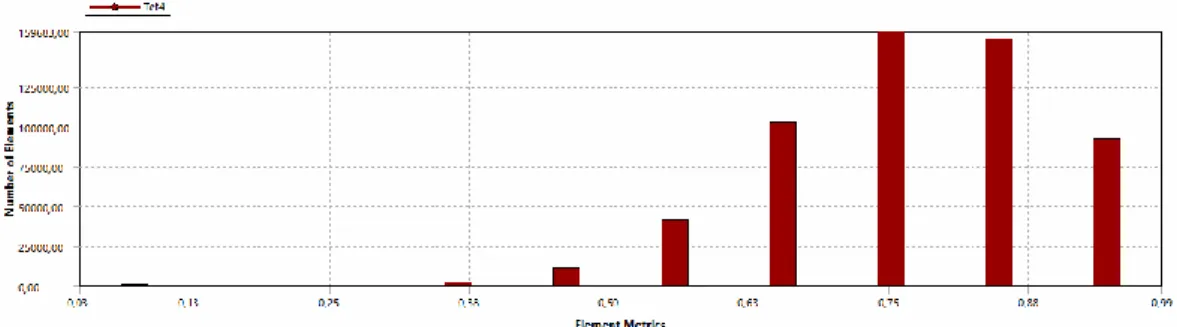
First, the material should be applied to the structure, which was defined in the last section. Then, a mesh with tetrahedron elements is created. The quality of the mesh is assessed by a mesh metric parameter which provides a value between 0 and 1 based on the geometry of the elements. In this scale, a value closer to 0 indicates lower element quality and a value closer to 1 indicates better element quality. This mesh metric used is “element quality” and it is based on the following expression:

𝑄𝑢𝑎𝑙𝑖𝑡𝑦 = 𝐶 [𝑣𝑜𝑙𝑢𝑚𝑒/√[[(𝑒𝑑𝑔𝑒 𝑙𝑒𝑛𝑔𝑡ℎ2_]3_{]] (3.10)}

The following table lists the value of C for each type of element.

Table 3.4 – Values of C for each type of element.

The criteria of quality mesh control is defined as 75% of the elements obtain a quality above of 75% and to prove the accuracy of the results is presented the percentage of stress error, in Chapter 4.

After meshing, BCs needed to be applied. For all the analysis, the BCs are the same, which are fixed support, on the faces where spars are intended. The fixed support has the objective of restricting the six degrees of freedom, which are translations and rotations in x, y, and z-axis. Pressure distribution is also applied around the wing surface. This last parameter comes from ANSYS Fluent.

As TO is done after structural analysis, it is not possible to considerer, in this dissertation, the large deflection, since ANSYS TO does not support a solution selection that has deformation turned on. Therefore, small deformation theory is used, i.e. displacements of the material particles are assumed to be much smaller than any relevant dimension of the body, so at each point of space can be assumed to be unchanged by the deformation.

The results of the equivalent stress, total deformation, and strain energy are presented in Chapter 4.

3.2.4 Topological Optimization

When meshing is done in Mechanical and loads are applied and evaluated, the topological optimization can be initiated. All steps in the process necessary to obtain the required results are explained below: analysis settings, optimization region, objective and response constraints.

3.2.4.1 Analysis Settings

In analysis settings, it is possible to define some input settings to the solver. The default maximum number of iterations is 500 but, according to the current problem’s objective, this value was set to 2000. The solver will iterate until it converges or until it reaches the maximum number of iterations.

The minimum normalized density is set to 0.001 which the program fully complies with, because for numerical reasons the density of an element cannot be equal to zero.

The convergence accuracy by default is set to 0.1%, but as the objective of this problem is to minimize the mass this value must be 0.05% or lower. The value chosen was 0.04%. The topological optimization solver will approach a stationary point where all constraints will be satisfied within a tolerance of 0.04% of the defined bound.

3.2.4.2 Optimization Region

The geometry to be optimized must be divided into design and exclusion region. The design region is the region that will be optimized, and the exclusion region is a fixed geometry and cannot be optimized by the solver.

In this work, the exclusion region is the wing surface, so the structure maintains the aerodynamic shape, and the spars, and the design region is the wing interior.

3.2.4.3 Response Constraints

The stress constraints are used to prevent the stresses at any point in the domain to exceed a stress level greater than half the yield strength of the material. The response constraint will be von-Mises yield criteria, with a maximum value of 36.5 MPa, which states that yielding occurs when the von Mises stress σvm equals the yield stress limit σlim. This yielding constraint is

necessary to enforce the assumption of linear elasticity. The von Mises is calculated for each element by the following equation [44]:

𝜎𝑣𝑚_𝑖=

1

√2√(𝜎𝑖1− 𝜎𝑖2)

2_{+ (𝜎}

𝑖2− 𝜎𝑖3)2+ (𝜎𝑖3− 𝜎𝑖1)2+ 6(𝜎𝑖42 + 𝜎𝑖52 + 𝜎𝑖62) (3.11)

where σi1-σi6 are the stress components for element i.

During the aircraft mission, the performance could not be affected, and so it is necessary to add to this problem the maximum deformation criterion. This constraint is applied on the z-axis, with a correspondent value of 0.1m, which was chosen as being 10% of the wingspan.

3.2.4.4 Objective

Weight reduction of structures is paramount in several industries due to its numerous benefits, such as lower consumption, performance gain and a reduction of material cost. The most common objective in topology optimization is to minimize compliance, which is the same as maximizing the stiffness. Although, in the present case studies the objective of TO problem is the mass minimization. However, weight reduction is constrained by several mechanical failure