Todos os direitos reservados.
É proibida a reprodução parcial ou integral do conteúdo
deste documento por qualquer meio de distribuição, digital ou
impresso, sem a expressa autorização do
REAP ou de seu autor.
Human Capital and the Recent Fall of
Earnings Inequality in Brazil
Priscilla Albuquerque Tavares
Naercio Aquino Menezes-Filho
HUMAN CAPITAL AND THE RECENT FALL OF
EARNINGS INEQUALITY IN BRAZIL
Priscilla Albuquerque Tavares
Naercio Aquino Menezes-Filho
Naercio Aquino Menezes Filho
Insper Faculdade de Economia, Administração e Contabilidade Rua Quatá, nº 300 Universidade de São Paulo (FEA/USP) Vila Olímpia
04546-042 - São Paulo, SP – Brasil
Priscilla Albuquerque Tavares Escola de Economia de São Paulo Fundação Getúlio Vargas (EESP/FGV) Rua Itapeva, nº 474
1
Human Capital and the Recent Fall of Earnings Inequality in Brazil
Priscilla Albuquerque Tavares
Sao Paulo School of Economics – FGV
Naercio Aquino Menezes-Filho
Insper and University of São Paulo
Abstract
Earnings inequality has started to fall in Brazil in recent years, after remaining very high for decades. We describe this decline using a flexible decomposition technique and assess the contributions of education and experience. We conclude that the fall in education earnings differentials and the decline in the dispersion within
demographic groups are the main factors leading to the reduction of inequality in Brazil. The paper demonstrates the powerful impact that education can have to reduce inequality.
Keywords: Human capital; income inequality; wages; education.
2
1. Introduction
Brazil has the world’s eighth largest economy (IMF, 2008). Nevertheless,
21.4% of the country’s people live in poverty, and 7.3% in misery (IPEADATA,
2009). This contradiction is the result of the country’s glaring income inequality
(UNDP, 2010)1. But, after decades remaining at a very high and stable level,
inequality has recently started to decline in Brazil and in several other
Latin-American countries (Lopez-Calva and Lustig, 2010). The aim of this paper is to
understand the reasons behind the fall of the Brazilian inequality, using a
flexible econometric approach and focusing on the role played by education
and age.
The focus of this paper is on observable skills because human capital is
one of the main determinants of earnings and therefore of earnings inequality.
Moreover, education has improved substantially in recent years in several Latin
American countries. Therefore, it is of interest to investigate whether the
decline of inequality is related to this education upgrade in Brazil, a major Latin
American country that has always been seen as very unequal.
The relation between education and inequality depends on two factors:
the education inequality among workers in the job market (composition effect)
and the monetary value the market attributes to each additional year of
schooling (price effect), as described by Ram (1990) and Knight and Salbot
(1983). In Brazil, both the education wage differentials and the great
educational disparity among workers have been traditionally important to
explain wage inequality (Lam and Levinson, 1992). In this paper we assess
what has been happening in recent years with the education inequality in Brazil
3
There is mounting evidence in the literature that the behavior of income
inequality is better explained by models that allow for wage changes that are
different for workers located in different points of the wage distribution. Autor et
al.(2005), for example, argue that the wage differentials in the upper part of the
distribution (90th/50th) have increased continuously since the 1970’s in the
United States, while in the bottom part (50/10) inequality increased in the
1980s, but has remained virtually unchanged since then. Corroborating these
results, Lemieux (2006a, 2006b) argues that changes in the returns to
measured skills have played a significant role in the growth of inequality since
the early 1970’s, but that the long-run increase in American income inequality is
concentrated in the upper part of the distribution and is basically due to the
rising returns to postsecondary education.
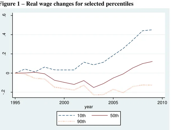
In Brazil, it is also very instructive to observe how earnings have changed
in the different parts of distribution. Figure 1 describes the evolution of real
wages since 1995 in Brazil in the 10th, 50th and 90th percentiles. Wages in 1995
are set to zero, so that the points in the figure are cumulative values with
respect to 1995. The figure shows, quite interestingly, that wages in the bottom
part of the distribution increased much more than in the median and in the top.
While wages at the 10th percentile grew by about 57%, median wages
increased 13% and wages at the 90th percentile actually fell in real terms.
In light of this scenario, in this article we examine the effects of changes in
the “composition” of workers’ attributes and their “prices” on income inequality
in Brazil between 1995 and 2009 using a quantile regression approach, which
4
distribution. This is in contrast with the recent literature that has examined the
issue of wage inequality in Latin America.
Ferreira, Leite and Litchfield (2008), for example, undertake a preliminary
investigation on the behavior of inequality in Brazil between 1981 and 2004,
focusing on the role played by inflation, but also examine the behavior of the
returns to education, rural-urban convergence and social assistance to the
poor. Manacorda, Sanchez-Paramo and Schady (2010) examine the behavior
of the returns to education in five Latin-American countries using a model of
demand for skills to find out that the rise in the supply of workers with
intermediate education has depressed wage differentials at this level. Neither
of these papers, however, decomposes the role played by human capital on
inequality into components between and within demographic groups at different
points of the earning distribution.2
This paper is organized as follows. The next section describes the data
and presents some descriptive evidence. Section 3 presents the econometric
methodology, while section 4 presents the econometric results. Section 5
5
2. Data
We use data from the National Household Survey (Pesquisa Nacional por
Amostra de Domicílios– PNAD/IBGE) from 1995 to 2009, conducted by the
Brazilian Institute of Geography and Statistics3. The worker sample consists of
men from 25 to 60 years old, with strictly positive principle job income and
workweek. We split the sample into 1980 cells, defined by the survey year,
worker age (in years) and education, grouped into four categories: zero to
three; four to seven; eight to 11 and 12 or more years of study. To measure
labor income we use the logarithm of real hourly wages, at 2005 prices (lw)4,
and our measures of inequality will be the variance of (log) wages, which is
perfectly decomposable. Table 1 presents the basic descriptive statistics of this
variable.
Figure 2 describes the evolution of the Gini coefficient calculated on the
basis of two different income measures: household per capita income and labor
market earnings. It shows that both measures of inequality fell substantially in
recent years, with respect to their 1995 level. Earnings inequality fell23.4%,
from an initial value of 0.394, while income inequality fell 10.6%,from a value of
0.600 in 1995. It seems, therefore, that in order to understand the reasons
behind the fall in overall inequality, it is important to grasp the determinants of
inequality in the labor market.
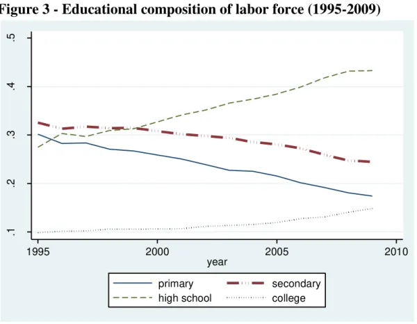
Between 1995 and 2009, the Brazilian labor force’s qualification increased
significantly, with the average schooling rising from 6.1 to eight years. Figure 3
describes the education composition of the workforce in Brazil over our sample
period. The share of the least educated (less than three years of education) fell
6
with high school education rose from 18% to 33%. The share of individuals with
college education rose from 9.8% to 14.2%. These are rapid changes for such
a small period of time and are likely to have an impact on the labor market and
inequality.
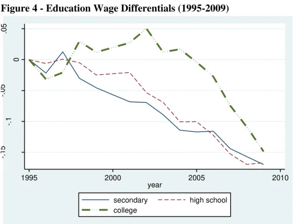
The impact of the changes in the education composition on the labor
market can be seen in Figure 4, where the behavior of the education wage
differentials over time is depicted. Returns to secondary education (with respect
to illiteracy) and to high school education have fallen quite substantially
between 1995 and 2009. Returns to college education, increased quite rapidly
between 1995 and 2003, but fell afterwards. Although we do not aim at
explaining the behavior of the education wage differentials in this paper, related
research shows that they reflect the evolution of the relative supply of different
education groups depicted above (Binelly, Meghir and Menezes-Filho, 2008).
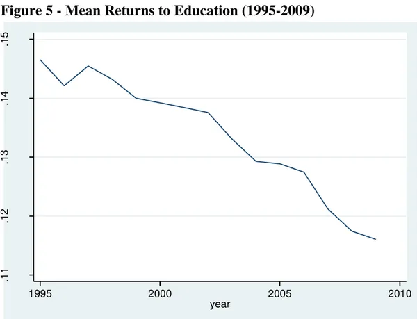
Figure 5 shows that behavior of the average returns to education in our
sample period. The returns have fallen almost continuously between 1995 and
2009, despite the rise in the college education wage differentials in the 1990s
documented above. This reflects the fact that the majority of the Brazilian
population has far less than college education, so that returns to more basic
education levels dominate the behavior of average returns.
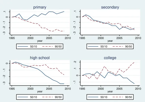
The behavior of wage inequality within the education groups is also of
substantial interest, as it allows us to infer the evolution of the demand for other
(unobserved) measures of skills. We can see from Figure 6 that both the 90th
-50th and the 50th-10th differentials have fallen for most education groups. The
exceptions are the 50th-10th differential in the primary education group and the
7
seems therefore that inequality is increasing in the top of the distribution, as it
has been happening in the USA (Lemieux, 2006a) and in the very bottom. In
what follows we attempt to describe this patterns using a flexible decomposition
8
3. Econometric Methodology
Our estimation model is based MaCurdy and Mroz (1995) and Goslin,
Machin and Meghir (2000), where log wage is described by polynomials of time
trends ( ), age ( ) and cohort ( ) effects and their interactions
R( ):
( ) ( ) ( ) ( ) (1)
where is a constant and is an error term. The time trends capture the
effects of interactions between changes in the demand and supply for the
different demographic groups, which may reflect skill biased technological
change, trade effects, etc. This term captures shocks on wage distribution that
are common within all educational groups, except by age factor, and is the only
form to take into account of life cycle differences on wage fluctuations across
generations.
The age and cohort effects capture the wage changes related to workers’
life cycle (age and experience) and specific generational characteristics
(different productive patterns and conditions when entering the job market). The
age functions measure wage distribution changes for specific educational group
in a given generation, and reflect life cycle wage changes unrelated to labor
market experience (one of the most important determinants of worker
productivity). The cohort functions measure wage differences between
generations related to different educational-specific cohort attributes, in terms
of unobserved ability. This factor is important once educational policy or
institutional labor market changes affect wage distribution and are difficult to
take into account. Given the existence of an exact linear relation between age,
9
coefficients of the cohort terms. Thus, the model now includes functions of age,
time trends and interactions between them only:
( ) ( ) ( ) (2)
We estimate this model for 21 log wage quantiles ( ), separately for the
four schooling groups6:
( ) ( ) ( ) (2’)
The interpretation of the components of the regression is simple: for a
given quantile of the distribution, differences of the coefficients of the functions:
( ) , ( ) and ( ) among education groups capture
changes in the return to education and experience and the interaction between
these two attributes. For a given education group, differences among the
coefficients of the functions: ( ) , ( ) and ( ) across
quantiles reflect changes in the intra-group wage dispersions. The estimated
quantile models give us the conditional distribution of log wages. From this
distribution it is possible to recover its unconditional distribution and decompose
the log wage variance, considering counterfactual exercises that explain the
different effects of education on wage inequality.
Hence, the decomposition of the variance consists of measuring the
portions of the wage dispersion attributed to the differences of workers’
productive attributes (between-group inequality) and the differences in
unobserved productive characteristics in the same group (within-group
inequality):
( ) ∑ ( ) ∑ [ ( ) ( )] (3)
where is the relative weight of cell in year ; ( ) and ( ) are the
10
are the mean and variance of log wages in the labor market in year . In
equation 3, the first term and the second term on the right-side refers to the
within-group and between-group dispersion, respectively.
The within-group variance is affected by changes in the labor force
composition and wage dispersion within each group of workers with the same
level of schooling and age. The inter-group or between-group variance, in turn,
is affected by the composition and the price effects of education and age. The
composition effect of education evaluates how changes in the educational
makeup of the workforce affect wage inequality over time. To estimate this
effect, we calculate the variance between groups, holding the wage returns to
education and experience and the age composition of the workers steady.
The price effect of education evaluates how changes in the differences in
wages paid to workers with different qualification levels affect wage inequality
over time. To estimate this effect, we calculate the inter-group component of
inequality, keeping the educational and age composition of the workers and the
wage returns to experience fixed. To maintain the returns to education and
experience fixed, we attribute zero to the trend and interaction terms of the
regression, before predicting the log wages. To keep the workforce composition
fixed, we maintain the relative weights of the education and age cells fixed at
their base-year levels (1995).
Therefore, the estimation procedure is done in two steps. In the first step
we estimate the log wage equations and obtain the conditional distributions of
log wages. In the second, we recover the unconditional distributions, for each
counterfactual exercise (price effect and composition effect). The procedures
11
First step – estimation: the models for the quantiles (2’) are estimated by
means of third-order polynomials in the functions for age, time and interactions:
(2’’)
The error term includes macroeconomic cyclical effects:
̅̅̅
These refer to the macroeconomic changes that occurred in a determined
period (such as changes in inflation, joblessness and economic activity) and
are orthogonal to the age and trend effects, that is, they do not include any
trends.7
The models are estimated by the smoothed least absolute deviations
method, which consists of a weighted least-squares estimator applied to the
context of quantile regressions, with desirable properties in small samples
(Horowitz, 1998). The coefficients are simply order statistics of each age, year
and education cell. The weights are based on the variance of each estimated
order statistic ( ̂ ), given by
(
̂
)
( )( ) , where is the number of
observations in cell and (
)
is the density of log wages in each cell at the qthquantile, estimated nonparametrically from a Gaussian kernel distribution:
( )
∑
(
̂)
, in whichis the logarithm of the wage of
each individual in the same cell
; is the fixed window (bandwidth) of half a
standard deviation of the log wages in each cell and ( ) is the standard
normal density function (Koenker and Portnoy, 1998).
This procedure is equivalent to choosing the vector of parameters that
12
( ̂ ) ( ̂ ) ( ̂ ) (4)
where is a set of linear restrictions that transforms the unrestricted model (1)
on restricted model (2).8 In our case, the restriction implies that the age, trend
and (orthogonal) time dummies are sufficient to explain the behavior of each
estimated statistic order across cells and over time. Imposing the restrictions
means estimating weighted least squares regressions on the grouped data, for
each quantile and education group separately. This procedure will give us
consistent estimates of . Under the null that the restrictions are valid, the
minimized value follows a chi-square distribution with degrees of freedom equal
to the number of restrictions. In order to construct the test statistics, we only
have to sum up the weighted squared residuals, that is, the estimated
percentiles minus the predicted values minus the orthogonal time dummies.
In the second step we recover the unconditional distribution: If and
correspond to a determined quantile of the unconditional and conditional wage
distributions, respectively, then ( ) and ( ), where
and . The relation between and is given by
∫
, where
is the relative size of cell and is the total number of cells, which can be
substituted by
∑
if the variables defining the cells are discrete.Given a set of predicted conditional quantiles , it can be estimated to which
conditional quantile of cell a given log wage level ( ) would correspond:
[ ( ) ( )
This procedure is carried out for the range of log wages observed in our
13
the 21 are found corresponding to the quantiles considered that
characterize the unconditional distribution, as well as this distribution’s mean
and variance. If ( ) ( ) is an accumulated density function,
then the empirical probability density function referring to quantile q can be
written as ( ) ( ) ( ), where is the neighboring
quantile. Thus, the mean and variance of the unconditional log wage
distribution are given by:
( ) ∑ ( )
and
( ) ∑[ ( )] ( )
The unconditional distributions are then obtained separately for each year,
considering each desired counterfactual exercise (fixing the wage returns or the
workforce composition).
This methodology can be seen as an extension of variance decomposition
traditional approach, wherein all log wage conditional distribution (beyond
conditional variance) can be recovered by innumerous quantiles non-linear
functions. The main advantage of this approach is provide a natural way to
decompose wage structure: composition effect is clearly interpreted as changes
on workers’ observable attributes and differences on quantiles can be seen as
an estimate of variations on wage non-observed component. But, this and other
decomposition methods do not allow establishing behavioral relationships or
find structural parameters. However, this descriptive methodology is useful to
quantify the contribution of different factors on wage distribution changes –
14
and shocks. Moreover, one convenience of using variance as inequality
measure is the possibilities of decomposition on between and within
components, that allow describe economic mechanisms as inducers of wage
inequality path changes – such as the rise of workers’ qualification and entry
15
4. Results
Tables 2a to 2c present the estimation results of the 25th, median, 75th
regressions for the different education groups, as examples of the patterns
found in the other percentiles. The trend, age and interaction terms are
statistically significant in most education groups. The differences in magnitude
of the trend coefficients among the quantiles in an education group evidence
changes in the wage distribution for workers with the same level of schooling
and experience. The interactions of trend and age reflect changes in the returns
to experience over time, which may also impact dispersion within groups. It is
easier to grasp the information contained in the estimated models by means of
graphs, however.
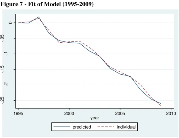
Figure 7 shows that changes in the variance predicted by the model
closely follows changes in the actual variance, computed using the individual
data. This demonstrates the model’s good fit and that the predicted variance
can be used to carry out the counterfactual exercises for the different effects of
education on wage inequality.
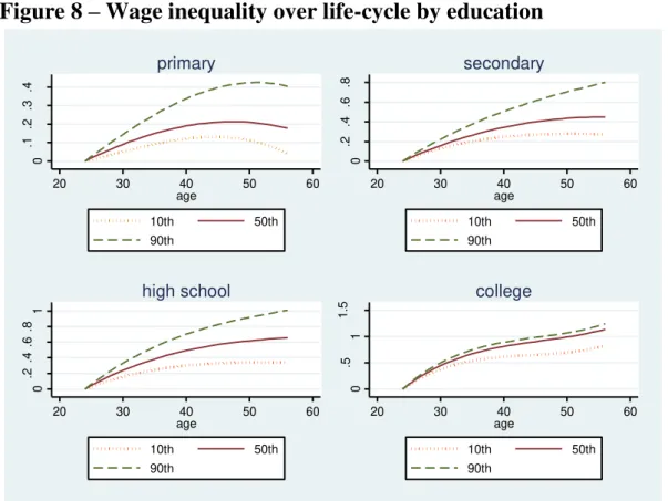
The differences in magnitude of the age coefficients across percentiles
and schooling groups reveal that returns to experience vary a great deal with
human capital and ability. Figure 8 shows that wage inequality increases with
age for all education groups, but this effect is much stronger for the less
educated. This indicates that there are unobserved productivity differences
across workers that are revealed on the job and that this heterogeneity is
higher among the less educated.
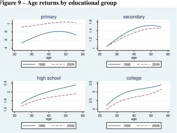
Figure 9 illustrates the behavior of wages over the life cycle for the
16
are higher for the more educated workers, indicating that returns to specific
human capital (on the job training) depend on general human capital. Over
time, returns to experience have flattened out for the high school and primary
educated workers, remaining stable for the other education groups. Therefore,
the decline of the returns to experience for less skilled and semi-skilled may
also have contributed to the fall in earnings dispersion, as we shall document
below.
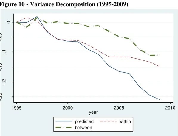
4.1 Variance Decomposition
Figure 10 documents the role played by the within and between-groups
components of wage inequality in Brazil over the past fifteen years. One can
notice that the behavior of overall inequality closely follows that of inequality
within-groups until 2001, with the between-group component remaining
basically constant until that year, meaning that most of the changes occur
within education and age cells. After 2001, however, inequality starts to fall
more rapidly than the within-groups component, due to the fall in the
between-groups component. In what follows, we try to disentangle the effects underlying
the behavior of this last component.
Figure 11 decomposes the between-group component into a price and a
composition effect. To calculate the composition effect we hold the wages for
each percentile in each cell constant at their 1995 level and allow the cell
weights to vary. To compute the price effect we hold the weights constant and
allow the wage differentials to move, as described in section 3 above. While the
composition effect contributes to the decrease in inequality after 1998, most of
17
especially after 2001. Moreover, most of this effect reflects the decline in the
education wage differentials, since holding the age differentials constant has
very little impact on the behavior of the price effects. It seems, therefore, that
the bulk of the decline in inequality between groups reflects the decline in the
education wage differentials.
4.2 Variance within-groups
Figure 12 plots the behavior of the within-groups component over time. It
is clear that its behavior reflected two forces acting in opposite directions. The
“pure” within-groups effect has shaped the overall declining trend of inequality
over time, but the composition effect (also called “mechanical” by Lemieux,
2006a) contributed to a continuous rise in inequality, since more educated and
older groups are more unequal. As a result, within-groups inequality fell less
rapidly then it would otherwise.
What other factors could explain the behavior of the within-groups
inequality? Aside from human capital, our regressions do not allow inferences
about other forces that can affect within-group variance. Nevertheless we can
speculate on some economic factors that can have affected wage inequality
within groups of workers with the same level of schooling in this period. One
possible explanation is the increase in the real value of the minimum monthly
wage that took place between 1995 and 2009. Figure 13 shows the minimum
wage almost doubled in our sample period, at the same time when inequality
within groups was falling substantially. Future research that can assess the
effects of minimum wage policy on earnings inequality is needed to investigate
18
Table 3 summarizes our main results by presenting the contribution of
each component to the reduction of inequality, year by year. The table shows
that the variance of wages declined by 0.25 between 1995 and 2009, from an
initial value of 0.93, that is, a reduction of 26%. Moreover, the reduction of the
education and age wage differentials accounts for about 44% of the total drop.
Changes in the education and age composition of the workforce explain about
eight percent of the change in inequality, as the new generations become
increasingly more educated. The contribution of the price effect within-groups is
in the range of 70%, the highest amongst all different factors. Finally, had all
the other forces remained constant, the higher human capital of the workforce
would have contributed to an increase in the overall variance of earnings by
about 22%, since inequality is higher among the more educated and
19
5. Conclusions
This paper evaluates the factors that have contributed to the decline in
earnings inequality in Brazil, for the first time in decades, by means of a flexible
decomposition technique and counterfactual exercises. The variance of (log)
earnings declined by about a quarter between 1995 and 2009. We find that,
until the end of the 1990s, most of the fall happened within education and age
groups, with very little role for our observable measures of skill. But, in the new
century, the between-groups component also contributed significantly to the fall
in inequality, mostly through the fall in the education wage differentials. Returns
to experience have also declined, especially among the less skilled workers.
We find that the education composition of the workforce also contributed
to the fall in inequality between groups, but increased the within-groups
dispersion. Overall, the results indicate the powerful impact that education can
20
References
AUTOR, D.H.; KATZ, L.F.; KEARNEY, M.S. (2005) “Rising Wage Inequality:
The Role of Composition and Prices”NBER Working Paper nº 11628.
BINELLI, C., MEGHIR, C.; MENEZES-FILHO, N. (2008) “Education and Wages
in Brazil”, University College London (mimeograph).
CHAMBERLAIN, G. (1993). “Quantile regressions, censoring and the structure
of wages”. Advances in Econometrics, 1.
CORSEUIL, C.H.; FOGUEL, M.N. (2002) “Uma sugestão de deflatores para
rendas obtidas a partir de algumas pesquisas domiciliares do IBGE”. IPEA
Discussion Paper nº 897.
FERREIRA, F.; LEITE, P.; LITCHFIELD, J. (2008). “The rise and fall of Brazilian
Inequality: 1981 – 2004”, Macroeconomic Dynamics, 12 199-230.
GOSLING, A.; MACHIN, S.; MEGHIR, C. (2000) “The Changing Distribution of
Male Wages in the UK”. The Review of Economic Studies, 67 (4); 635-66.
HOROWITZ, J.L. (1998) “Bootstrap Methods for Median Regression Models”.
Econometrica, 66 (6); 1327-1351.
IBGE. Pesquisa Nacional por Amostra de Domicílios. Brazilian Geography and
Statistics Institute.
IPEADATA. Brazilian Applied Economics Research Institute.
INTERNATIONAL Monetary Fund. (2008) World Economic Outlook Database.
KNIGHT, J.; SALBOT, R. (1983) “Education Expansion and the Kuznets Effect”.
American Economic Review, 73; 1132-36.
KOENKER, R.; PORTNOY, S. (1998) “Quantile Regressions” University of
21
LAM, D.; LEVINSON, D. (1992) “Declining inequality in schooling in Brazil and
its effects on inequality in earnings”. Journal of Development Economics, 37
(2), 199-225.
LEMIEUX, T. (2002) “Decomposing Changes in Wage Distributions: A Unified
Approach”. Canadian Journal of Economics, 35 (4), 646-88.
LEMIEUX, T. (2006a) “Increasing Residual Wage Inequality: Composition
Effects, Noisy Data, or Rising Demand for Skill?”American Economic Review,
96 (3), 461-98.
LEMIEUX, T. (2006b) “Post-secondary Education and Increasing Wage
Inequality”. American Economic Review, 96 (3), 1-23.
LOPEZ-CALVA, L. AND LUSTIG, N. (2010) Declining Inequality in Latin
America: A Decade of Progress”. UNDP: New York.
MACURDY, T.; MROZ, T., (1995) “Estimating Macro Effects from Repeated
Cross-Sections”, Stanford University Discussion Paper.
MANACORDA, M; SANCHEZ-PARAMO; C. AND SCHADY, N. (2010)
“Changes in Returns to Education in Latin America: The Role of Demand and
Supply of Skills”, Industrial and Labor Relations Review, 63.
MENEZES-FILHO, N.; FERNANDES, R.; PICCHETTI, P. (2006) “Rising Human
Capital but Constant Inequality: The education composition effect in Brazil”
Revista Brasileira de Economia, 60 (4); 407-24.
RAM, R. (1990) “Education expansion and schooling inequality: International
evidence and some implications”. Review of Economics and Statistics 72,
266-73.
ROTHENBERG, T. (1971). Efficient Estimation with a Priori Information. Yale
22
UNITED NATIONS DEVELOPMENT PROGRAMME (2010). Human
Development Report. New York.
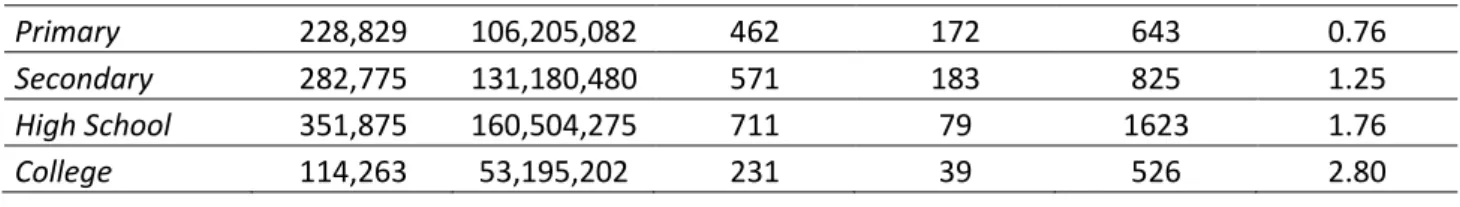
Table 1
–
Data Description
Education group Number of observations
Population represented
Mean number of
cell observations
Minimum number of
cell observations
Maximum number of
cell observations
Median of the real log hourly wage
Primary 228,829 106,205,082 462 172 643 0.76
Secondary 282,775 131,180,480 571 183 825 1.25
High School 351,875 160,504,275 711 79 1623 1.76
College 114,263 53,195,202 231 39 526 2.80
Source: 1995 to 2009 PNADs.
23
Table 2a
Regression Coefficients - Quantile 25
Primary Secondary High School College
Trend -0.19* -0.28* -0.27* -0.50*
(0.06) (0.05) (0.05) (0.12)
Trend2 0.13 0.12 -0.10 0.29***
(0.09) (0.08) (0.08) (0.17)
Trend3 0.13* 0.15* 0.21* -0.04
(0.04) (0.03) (0.03) (0.07)
Age 0.07** 0.29* 0.45* 0.93*
(0.03) (0.02) (0.02) (0.06)
Age2 0.00 -0.04* -0.11* -0.36*
(0.02) (0.02) (0.02) (0.03)
Age3 0.00 0.00 0.01** 0.05*
(0.00) (0.00) (0.00) (0.01)
Trend*Age 0.07** -0.11* -0.10* -0.10***
(0.03) (0.03) (0.03) (0.06)
Trend2*Age -0.01 0.02*** 0.01*** 0.04*
(0.01) (0.01) (0.01) (0.01)
Trend*Age2 -0.02 0.00 0.01 -0.02
(0.02) (0.01) (0.02) (0.03)
Constant 0.20* 0.61* 1.03* 1.80*
(0.02) (0.01) (0.01) (0.03)
Chi-square test 583.57 498.56 541.82 739.16
P-value 0.00 0.45 0.07 0.00
Source: 1995 to 2009 PNADs. Notes: *p>0.01; **p>0.05; ***p>0.10.
Number of observations: 495 cells. Primary: zero to three years of schooling;
24
Table 2b
Regression Coefficients - Median
Primary Secondary High School College
Trend -0.20* -0.34* -0.46* -0.30*
(0.05) (0.05) (0.05) (0.10)
Trend2 0.18** -0.01 -0.07 -0.02
(0.07) (0.07) (0.07) (0.15)
Trend3 0.12* 0.19* 0.23* 0.06
(0.03) (0.03) (0.03) (0.06)
Age 0.25* 0.36* 0.50* 0.98*
(0.02) (0.02) (0.02) (0.05)
Age2 -0.05* -0.07* -0.12* -0.36*
(0.01) (0.02) (0.02) (0.03)
Age3 0.00 0.00 0.01* 0.05*
(0.00) (0.00) (0.00) (0.01)
Trend*Age -0.11* -0.08* -0.02 -0.08
(0.03) (0.03) (0.03) (0.06)
Trend2*Age 0.03* 0.02* 0.01*** 0.02
(0.01) (0.01) (0.01) (0.01)
Trend*Age2 -0.01 0.00 -0.04* 0.01
(0.01) (0.01) (0.01) (0.03)
Constant 0.54* 1.06* 1.52* 2.26*
(0.01) (0.01) (0.01) (0.03)
Chi-square test 402.86 556.92 500.13 621.37
P-value 1.00 0.03 0.43 0.00
Source: 1995 to 2009 PNADs. Notes: *p>0.01; **p>0.05; ***p>0.10.
25
Table 2c
Regression Coefficients - Quantile 75
Primary Secondary High School College
Trend -0.20* -0.48* -0.53* -0.13
(0.06) (0.06) (0.06) (0.11)
Trend2 -0.14 0.08 -0.08 -0.21
(0.08) (0.08) (0.09) (0.15)
Trend3 0.26* 0.16* 0.21* 0.11
(0.04) (0.04) (0.04) (0.07)
Age 0.32* 0.44* 0.56* 1.02*
(0.03) (0.03) (0.03) (0.05)
Age2 -0.06* -0.09* -0.11* -0.39*
(0.02) (0.02) (0.02) (0.03)
Age3 0.00 0.00 0.01 0.06*
(0.00) (0.00) (0.00) (0.01)
Trend*Age -0.06 -0.10* 0.01 -0.04
(0.03) (0.03) (0.03) (0.06)
Trend2*Age 0.02* 0.02* 0.01 -0.01
(0.01) (0.01) (0.01) (0.01)
Trend*Age2 -0.01 -0.01 -0.04 0.05
(0.02) (0.02) (0.02) (0.03)
Constant 1.02* 1.47* 2.00* 2.72*
(0.02) (0.01) (0.02) (0.03)
Chi-square test 476.59 638.61 570.14 638.79
P-value 0.72 0.00 0.01 0.00
Source: 1995 to 2009 PNADs. Notes: *p>0.01; **p>0.05; ***p>0.10.
26
Table 3
Contribution of Each Component to the Reduction of Inequality
Year Variance
changes
Between component
(prices) %
Between component (composition)%
Within component
(prices) %
Within component (composition)%
1996 0,01 -3,00 0,60 1,65 1,63
1997 0,02 0,38 0,14 0,20 0,29
1998 -0,03 0,09 -0,12 1,60 -0,50
1999 -0,05 -0,11 -0,01 1,42 -0,26
2000 -0,05 0,09 0,02 1,25 -0,32
2001 -0,06 0,10 0,04 1,19 -0,31
2002 -0,09 0,19 0,05 1,09 -0,28
2003 -0,11 0,15 0,08 1,06 -0,26
2004 -0,14 0,22 0,06 0,96 -0,20
2005 -0,16 0,29 0,07 0,86 -0,20
2006 -0,17 0,33 0,09 0,83 -0,23
2007 -0,21 0,41 0,09 0,70 -0,20
2008 -0,23 0,44 0,08 0,70 -0,22
2009 -0,25 0,44 0,08 0,71 -0,22
27
Figure 1
–
Real wage changes for selected percentiles
Source: 1995 to 2009 PNADs.
Note: Cumulative changes in the logarithm of real hourly wages (2005 prices) with respect to 1995.
Figure 2 - Gini Index - Per capita family income and Earnings
Sources: PNADS 1995 to 2009 and IPEADATA.
-.
2
0
.2
.4
.6
1995 2000 2005 2010
year
10th 50th
90th
-.
1
-.
0
5
0
1995 2000 2005 2010
year
28
Figure 3 - Educational composition of labor force (1995-2009)
Source: PNADS 1995 to 2009.
Notes: (a) Male workers aged 24 to 56; (b) Education groups: primary – zero to three years of schooling; secondary – four to seven years of schooling; high school – eight to 11 years of schooling; college – 12 or more years of schooling.
.1
.2
.3
.4
.5
1995 2000 2005 2010
year
primary secondary
29
Figure 4 - Education Wage Differentials (1995-2009)
Source: 1995 to 2009 PNADs.
Note: Cumulative change in log wage differentials with respect to the previous education groups. Education groups: primary – zero to three years of schooling; secondary – four to seven years of schooling; high school – eight to 11 years of schooling; college – 12 or more years of schooling.
-.
1
5
-.
1
-.
0
5
0
.0
5
1995 2000 2005 2010
year
secondary high school
30
Figure 5 - Mean Returns to Education (1995-2009)
Source: 1995 to 2009 PNADs.
Note: Regression coefficients of the logarithm of real hourly wages (2005 prices) against years of schooling, age and age squared.
.1
1
.1
2
.1
3
.1
4
.1
5
1995 2000 2005 2010
31
Figure 6
–
Within variance by educational group
Source: 1995 to 2009 PNADs.
Note: Cumulative changes in the logarithm of real hourly wages
differentials with respect to 1995. Education groups: primary – zero to three years of schooling; secondary – four to seven years of schooling; high school – eight to 11 years of schooling; college – 12 or more years of schooling. -. 3 -. 2 -. 1 0 .1
1995 2000 2005 2010
year 50/10 90/50 primary -. 3 -. 2 -. 1 0 .1
1995 2000 2005 2010
year 50/10 90/50 secondary -. 3 -. 2 -. 1 0
1995 2000 2005 2010
year 50/10 90/50 high school -. 1 0 .1 .2
1995 2000 2005 2010
year
50/10 90/50
32
Figure 7 - Fit of Model (1995-2009)
Source: 1995 to 2009 PNADs.
Note: Cumulative change in the variance of the logarithm of real hourly wages with respect to 1995.
-.
2
5
-.
2
-.
1
5
-.
1
-.
0
5
0
1995 2000 2005 2010
year
33
Figure 8
–
Wage inequality over life-cycle by education
Source: 1995 to 2009 PNADs.
Note: Cumulative changes in the logarithm of real hourly wages (2005 prices) with respect to age 25 by education group.
0
.1
.2
.3
.4
20 30 40 50 60
age 10th 50th 90th primary 0 .2 .4 .6 .8
20 30 40 50 60
age 10th 50th 90th secondary 0 .2 .4 .6 .8 1
20 30 40 50 60
age 10th 50th 90th high school 0 .5 1 1 .5
20 30 40 50 60
age
10th 50th
90th
34
Figure 9
–
Age returns by educational group
Source: 1995 to 2009 PNADs.
Note: Predicted logarithm of real hourly wages (2005 prices), by educational group.
.4
.6
.8
1
20 30 40 50 60
age 1995 2009 primary 1 1 .2 1 .4 1 .6
20 30 40 50 60
age 1995 2009 secondary 1 .2 1 .6 2 2 .4
20 30 40 50 60
age 1995 2009 high school 2 2 .5 3 3 .5
20 30 40 50 60
age
1995 2009
35
Figure 10 - Variance Decomposition (1995-2009)
Source: 1995 to 2009 PNADs.
Note: Cumulative change in the within-group and between-group components of the variance of the logarithm of real hourly wages (2005 prices) with respect to 1995.
-.
2
5
-.
2
-.
1
5
-.
1
-.
0
5
0
1995 2000 2005 2010
year
predicted within
36
Figure 11 - Between group variance component (1995-2009)
Source: 1995 to 2009 PNADs.
Note: Cumulative change in the price and composition effects of the between-groups variance of the logarithm of real hourly wages (2005 prices) with respect to 1995. Composition effect: Wage inequality due to the changes in educational and labor force age compositions (wage returns fixed at 1995 level). Price effect: Wage inequality due to changes in wage returns (educational and age compositions fixed at 1995 levels).
-.
1
-.
0
5
0
.0
5
1995 2000 2005 2010
year
between prices
37
Figure 12 - Within group variance component (1995-2009)
Source: 1995 to 2009 PNADs.
Note: Cumulative change in the within groups components of the
variance of the logarithm of real hourly wages (2005 prices) with relation to 1995. Composition effect: Intra-group wage inequality due to changes in the educational and age compositions of the labor force (intra-cell variances fixed at 1995 levels). Intra-cell variance effect: Intra-group wage inequality due to changes in the intra-cell variances of education (educational and age compositions fixed at 1995 levels).
-.
2
-.
1
5
-.
1
-.
0
5
0
.0
5
1995 2000 2005 2010
year
within variance
38
Figure 13 - Minimum wage and wage inequality (1995-2009)
Sources: PNADS 1995 to 2009 and IPEADATA. Note: Real minimum wage, in Brazilian currency (Real, R$).
1
In a comparison with 126 countries, Brazil is the 10th most unequal. 2
Menezes-Filho, Fernandes and Picchetti (2006) used a similar methodology to decompose the evolution of inequality in Brazil between 1981 and 1997, before inequality started to fall. 3
For 1991, 1994 and 2000, when the PNAD was not conducted, we interpolated the variables using the simple average of the two adjacent years.
4
We used the income deflator of Corseuil and Foguel (2002).
5The worker’s age is determined by the survey year less the birth cohort (i = t – c). 6
1st, 5th, 10th, 15th, 20th, 25th, 30th, 35th, 40th, 45th, 50th, 55th, 60th, 65th, 70th, 75th, 80th, 85th, 90th, 95th and 99th.
7
See MaCurdy e Mroz (1995) 8
See Rothenberg (1971) and Chamberlain (1993).
2 5 0 3 0 0 3 5 0 4 0 0 4 5 0 5 0 0 mi n imu m w a g e .5 .5 5 .6 .6 5 .7
1995 2000 2005 2010
year