FRACTIONAL CENTRED DERIVATIVES
MANUEL DUARTE ORTIGUEIRAReceived 2 January 2006; Revised 4 May 2006; Accepted 7 May 2006
Fractional centred differences and derivatives definitions are proposed, generalizing to real orders the existing ones valid for even and odd positive integer orders. For each one, suitable integral formulations are obtained. The computations of the involved integrals lead to new generalizations of the Cauchy integral derivative. To compute this integral, a special two-straight-line path was used. With this the referred integrals lead to the well-known Riesz potential operators and their inverses that emerge as true fractional centred derivatives, but that can be computed through summations similar to the well-known Gr¨unwald-Letnikov derivatives.
Copyright © 2006 Hindawi Publishing Corporation. All rights reserved.
1. Introduction
Fractional calculus has been emerging as a very interesting tool for an increasing num-ber of scientific fields, namely, in the areas of electromagnetism, control engineering, and signal processing. However, an interested scientist or engineer has to face the problem created by the somewhat chaotic state of the art due to the existence of several definitions that lead to different results: Riemann-Liouville, Caputo, Gr¨unwald-Letnikov, Hadamard, Marchaud, are some of the known definitions [9–11]. Motivated by signal processing ap-plications, we should accept only the definitions that might lead to a fractional systems theory coherent with the usual practice and accepted notions and concepts. For this goal we have been proposing approaches for a coherent basis of the fractional calculus [5,7–9]. Namely, in [5,7,8], we assumed as a starting point the definitions of forward and back-ward fractional differences and their integral representations. From these representations and using the asymptotic properties of the Gamma function, we obtained a generalized Cauchy integral as a unified formulation for any order derivative. When computing the Cauchy integral using the Hankel contour, we obtained a regularized integral, generaliz-ing the well-known concept of pseudofunction, but without rejectgeneraliz-ing any infinite part. The notions of forward and backward derivatives emerged as very special cases. Their study for the case of functions with Laplace transforms led to defining causal and anti-causal Liouville differintegrations [7].
Hindawi Publishing Corporation
International Journal of Mathematics and Mathematical Sciences Volume 2006, Article ID 48391, Pages1–12
In the same line of thoughts we present here a similar procedure, but using centred fractional differences as starting points.
We proceed according to the following steps.
(i) Introduce the general framework for the centred differences, considering two cases that we will call type 1 and type 2. These are generalizations of the usual centred differences for even and odd positive orders, respectively.
(ii) For those differences, integral representations will be presented. (iii) These differences lead to Gr¨unwald-Letnikov-like centred derivatives.
(iv) From the integral representations we obtain generalizations of the Cauchy deriv-ative integral.
(v) If the integration is performed over a two-straight-line path that “closes” at in-finity, those integrals lead to the Riesz potentials and inverses.
A very important feature of the theory lies in the bridge it establishes between the Gr¨unwald-Letnikov-like centred derivatives that are summation formulae and the Riesz potentials and inverses.
We must refer that we will not address the existence problem. We are mainly interested in obtaining a coherent formulation.
The paper outline is as follows. InSection 2we revise the previously published the-ory. InSection 3we present the type 1 and type 2 centred differences and their integral representations. Centred derivative definitions similar to Gr¨unwald-Letnikov ones and their integral representations obtained generalizing the Riesz potentials and inverses are presented inSection 4. At last we present some conclusions.
Caution 1.1. In this paper, we deal with a multivalued expressionzαfrequently. Unless explicitly stated we will choose the negative real half-axis as branch cut line and assume that the obtained function is continuous above it. With this, we will write (−1)α=eiαπ.
2. Previous work
Let f(z) be a complex variable function and introduce the “forward” and “backward” (we use these terms with meanings coherent with the signal processing usage: forward means the use of the past and present values, while backward refers to the use of present and future values) fractional order differences defined by
∆αdf(z)=
∞
k=0
(−1)k
α k
f(z−kh),
∆α
rf(z)=(−1)α
∞
k=0
(−1)k
α k
f(z+kh),
(2.1)
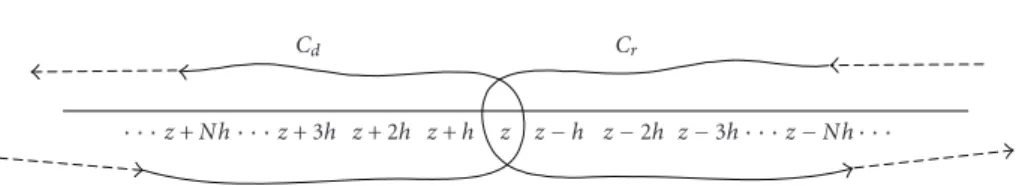
z+Nh z+ 3h z+ 2h z+h z z h z 2h z 3hz Nh
Cd Cr
Figure 2.1. Integration paths and poles for the integral representation of fractional order differences.
Gr¨unwald-Letnikov derivatives:
Dαdf(z)= lim h→0+
∞
k=0(−1)k
α k
f(z−kh)
hα ,
Dα
rf(z)= lim h→0+(−1)
α
∞
k=0(−1)k
α k
f(z+kh)
hα .
(2.2)
It is interesting to remark that these definitions were proposed first by Liouville [2]. Assuming thatf(z) is analytic inside and on an infinite integration path that encircles the pointst=z−khin the forward case andt=z+khin the corresponding backward case, withk∈Z+0, it is possible to use the residue theorem to obtain integral representa-tions for the differences [5,8] (seeFigure 2.1). However, with a translation we can obtain simpler representations with poles at +khand−kh, withk∈Z+0, respectively,
∆αdf(z)=
Γ(α+ 1) 2πih
Cd
f(z+w) Γ(w/h) Γ(w/h+α+ 1)dw,
∆αrf(z)=
(−1)α+1Γ(α+ 1)
2πih
Cr
f(z+w) Γ(−w/h) Γ(−w/h+α+ 1)dw.
(2.3)
For the computation of the limit ash goes to zero inside the above integrals we used the asymptotic properties of the ratio of two gamma functions (see later) to obtain the generalized Cauchy integral
Dαf(z)=Γ(α+ 1) 2πi
Cf(z+w) 1
wα+1dw, (2.4)
whereC is any U-shaped contour that encircles the branch cut line ofw−α−1 starting
at w=0 and staying on the left or on the right depending on the derivative we want; forward or backward. With the choice of the Hankel contour as a special integration path we obtain a regularized derivative:
Dαf(z)=ei(π−θ)α Γ(−α)
∞
0
f(x·eiθ+z)−N
0 (f(n)(z)/n!)einθxn
xα+1 dx, (2.5)
Iff(t) has (two-sided) Laplace transforms, the referred derivatives read, respectively,
Dαdf(t)= 1 Γ(−α)
∞
0 f(t
−τ)·τ−α−1dτ,
Dατf(t)= (−1)−α
Γ(−α)
∞
0 f(t+τ)
·τ−α−1dτ.
(2.6)
These derivatives were introduced both exactly with this format by Liouville [2]. The first is essentially a causal derivative while the second is anticausal. Both are suitable for defining fractional linear systems [7,10].
3. Centred differences and derivatives
3.1. Integer-order centred differences and derivatives. We introduce∆cas finite “cen-tred” difference defined by [6]
∆cf(t)=f
t+h 2
−f
t−h 2
. (3.1)
By repeated application, we have
∆Ne f(z)= N/2
k=−N/2
(−1)N/2−k N!
(N/2 +k)!(N/2−k)!f(t−kh) (3.2)
whenNis even, and
∆N0 f(t)=
N/2
k=−N/2
(−1)N/2−k N!
(N/2 +k)!(N/2−k)!f(t−kh) (3.3)
ifNis odd and whereN/k=−2N/2means that the summation is done over half-integer values.
Using the Gamma function, we can rewrite the above formulae in the format stated as follows.
Definition 3.1. LetNbe a positive even integer. Define a centred difference by
∆N
e f(t)=(−1)N/2 N/2
k=−N/2
(−1)k Γ(N+ 1)
Γ(N/2 +k+ 1)Γ(N/2−k+ 1)f(t−kh). (3.4)
Definition 3.2. LetNbe a positive odd integer. Define a centred difference by
∆N
0 f(t)=(−1)(N+1)/2 (N+1)/2
k=−(N−1)/2
(−1)k
× Γ(N+ 1)
Γ
(N+ 1)/2−k+ 1 Γ
(N−1)/2 +k+ 1f
t−kh+h 2
.
(3.5)
Definition 3.3. LetNbe a positive even integer. Define a centred derivative by
DeNf(t)=lim h→0
∆N e f(t)
hN =limh→0 (−1)N/2
hN N/2
k=−N/2
(−1)k Γ(N+ 1)
Γ(N/2 +k+ 1)Γ(N/2−k+ 1)f(t−kh). (3.6)
Definition 3.4. LetNbe a positive odd integer. Define a centred derivative by
DN
0 f(t)=lim
h→0
∆N0 f(t)
hN =limh→0
(−1)(N+1)/2
hN
(N+1)/2
k=−(N−1)/2
(−1)k
× Γ(N+ 1)
Γ
(N+ 1)/2−k+ 1 Γ
(N−1)/2 +k+ 1f
t−kh+h 2
.
(3.7)
Both derivatives (3.6) and (3.7) coincide with the usual derivative.
3.2. Fractional-order centred differences. Here we follow the steps of the previous sec-tion and introduce two types of fracsec-tional centred differences. Letα >−1,h∈R+, and
f(t) a complex variable function.
Definition 3.5. Define a type 1 fractional difference by
∆α c1f(t)=
+∞
−∞
(−1)kΓ(α+ 1)
Γ(α/2−k+ 1)Γ(α/2 +k+ 1)f(t−kh). (3.8)
Letα=2M,M∈Z+, in the first. Obtain
∆2M c1 f(t)=
+M
−M
(−1)k(2M)!
(M−k)!(M+k)!f(t−kh), (3.9)
that, aside a factor (−1)M, it is the above 2Morder centred difference. Definition 3.6. Define a type 2 fractional difference by
∆α c2f(t)=
+∞
−∞
(−1)kΓ(α+ 1) Γ (α+ 1)/2−k+ 1
Γ (α−1)/2 +k+ 1f
t−kh+h 2
. (3.10)
Similarly, ifαis odd (α=2M+ 1), it is, aside the factor (−1)M+1, equal to current centred
difference. In fact,
∆2c2M+1f(t)= M+1
−M
(−1)k(2M+ 1)! (M+ 1−k)!(M+k)!f
t−kh+h 2
. (3.11)
In particular, withM=0, obtain
∆1c2f(t)=f
t+h 2
−f
t−h 2
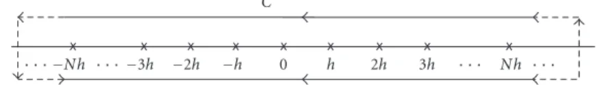
Nh 3h 2h h 0 h 2h 3h Nh
C
Figure 3.1. Integration path and poles for the integral representation of type 1 differences.
With the following relation [1]:
+∞
−∞
1
Γ(a−k+ 1)Γ(b−k+ 1)Γ(c+k+ 1)Γ(d+k+ 1)
= Γ(a+b+c+d+ 1)
Γ(a+c+ 1)Γ(b+c+ 1)Γ(a+d+ 1)Γ(b+d+ 1)
(3.13)
valid fora+b+c+d >−1, it is not very hard to show that
∆βc1
∆αc1f(t)
=∆αc1+βf(t),
∆βc2
∆α c2f(t)
= −∆αc1+βf(t),
(3.14)
while
∆βc2
∆α c1f(t)
=∆αc2+βf(t), (3.15)
provided thatα+β >−1. In particular,α+β=0, and the relations (3.14) show that when |α|<1 and|β|<1, the inverse differences exist and can be obtained by using formulae (3.8) and (3.10). We must remark that the zero-order difference is the identity operator and is obtained from (3.8). It is interesting to remark that the combination of equal types of differences gives a type 1 difference, while the combination of different types gives a type 2 difference. When comparing these differences with (3.2) and (3.3), we see that a power of−1 was removed. In a latter section we will understand why.
3.3. Integral representations for the fractional centred differences. Let us assume that
f(z) is analytic in a region of the complex plane that includes the real axis. Assume that
αis not an integer. To obtain the integral representations for the previous differences we follow here the procedure used in [5–8]. It can be easily verified that
∆αc1f(t)=
Γ(α+ 1) 2πih
Cf(z+w)
Γ(−w/h+ 1)Γ(w/h) Γ(−w/h+α/2 + 1
Γ
w/h+α/2 + 1dw. (3.16)
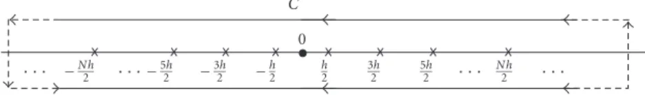
Nh 2
5h 2
3h 2
h 2
0 h 2
3h 2
5h 2
Nh 2
C
Figure 3.2. Integration path and poles for the integral representation of type 2 differences.
Regarding the second case, the poles are located now at the half-integer multiples ofh
(seeFigure 3.2), which leads to
∆αc2f(t)=
Γ(α+ 1) 2πih
CC
f(z+w) Γ
−w/h+ 1/2 Γ
w/h+ 1/2 Γ
−w/h+α/2 + 1 Γ
w/h+α/2 + 1dw. (3.17)
These integral formulations will be used in the following section to obtain the integral formulae for the centred derivatives.
4. Fractional centred derivatives
4.1. Definitions. To obtain fractional centred derivatives (Gr¨unwald-Letnikov like) we proceed as usual [7,10,11]: divide the fractional differences byhα(h∈R+) and leth→0.
Definition 4.1. For the first case, and assuming again thatα >−1, define the type 1 frac-tional centred derivative:
Dα
c1f(t)=lim h→0
∆α c1f(t)
hα =limh→0
Γ(α+ 1)
hα
+∞
−∞
(−1)k
Γ(α/2−k+ 1)Γ(α/2 +k+ 1)f(t−kh). (4.1)
Definition 4.2. For the second case, define the type 2 fractional centred derivative given by
Dαc2f(t)=lim h→0
∆α c2f(t)
hα
=lim h→0
Γ(α+ 1)
hα
+∞
−∞
(−1)k Γ (α+ 1)/2−k+ 1
Γ (α−1)/2 +k+ 1f
t−kh+h 2
.
(4.2)
Formulae (4.1) and (4.2) generalize the positive-integer-order centred derivatives to the fractional case, although there should be an extra factor (−1)α/2in the first case and
(−1)(α+1)/2in the second case that we removed. It is a simple task to obtain the derivative
analogues to (3.14) and (3.15). In fact we have
Dβc1
Dα c1f(t)
=Dαc1+βf(t),
Dcβ2
Dα c2f(t)
= −Dαc1+βf(t),
while
Dβc2
Dα c1f(t)
=Dαc2+βf(t) (4.4)
again withα+β >−1.
4.2. Integral formulae. To obtain the integral formulae for the derivatives, we must sub-stitute the integral formulae (3.16) and (3.17) into (4.1) and (4.2), respectively, and per-mute there the limit and integral operations. With this permutation we must compute the limit of two quotients of Gamma functions. As it is well known, the quotient of two gamma functionsΓ(s+a)/Γ(s+b) has an interesting expansion [3,11]:
Γ(s+a) Γ(s+b)=s
a−b
1 + N
1
cks−k+Os−N−1
(4.5)
as|s| → ∞, uniformly in every sector that excludes the negative real half-axis. Whenhis very small,
Γ(w/h+a) Γ(w/h+b)≈
w
h
a−b
1 +h·φ
w
h
, (4.6)
whereϕis regular near the origin. According to the above statement, the branch cut line used to define a function on the right-hand side of (4.6) is the negative real half axis. Similarly, we have
Γ(−w/h+a) Γ(−w/h+b)≈
−w h
a−b
1 +h·φ
−w h
, (4.7)
but now, the branch cut line is the positive real axis. With these results, we obtain the following.
Theorem4.3. In the above conditions, the integral formulation for type1derivative is
Dαc1f(t)=
Γ(α+ 1) 2πi
Cc
f(z+w) 1
(w)α/12+1(−w)α/r 2dw, (4.8) while for type2derivative, it is
Dα c2f(t)=
Γ(α+ 1) 2πi
Cc
f(z+w) 1
(w)(1α+1)/2(−w) (α+1)/2
r
dw. (4.9)
The subscripts “l” and “r” mean, respectively, that the power functions have the left and right half real axis as branch cut lines. These integrals represent again generalizations of the Cauchy derivative.
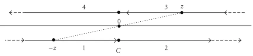
Now, we are going to compute the above integrals for the special case of straight line paths. Let us assume that the distance between the horizontal straight lines in Figures2.1
1 2 3 4
0
z
z
C
Figure 4.1. Segments for the computation of the integrals in (4.8) and (4.9).
used for the computation of the above integrals. If we assume that the two-straight-lines are infinitely near, we have for type 1 derivative
1
= −Γ(α+ 1) 2πi
∞
0 f(z
−x) 1
xα+1e−iαπ/2e−iπe
−iπdx,
2
=Γ(α+ 1) 2πi
∞
0 f(z+x)
1
xα+1eiαπ/2dx,
3
= −Γ(α+ 1)e −iαπ/2
2πi
∞
0 f(z+x)
1
xα+1e−iαπ/2dx,
4
=Γ(α+ 1) 2πi
∞
0 f(z
−x) 1
xα+1eiαπ/2eiπe iπdx,
(4.10)
where the integer refers the straight-line segment used in the computation. Joining the four integrals, we obtain
Dα
c1f(t)= −
Γ(α+1) sin(απ/2)
π
∞
0 f(z
−x) 1
xα+1dx
−Γ(α+ 1) sin(απ/2) π
∞
0 f(z+x)
1
xα+ 1dx
(4.11)
or
Dαc1f(t)= −
Γ(α+ 1) sin(απ/2)
π
∞
−∞f(z
−x) 1
|x|α+1dx. (4.12)
Asαis not an odd integer that we obtain and using the reflection formula of the gamma function, we obtain
Dcα1f(t)=
1
2Γ(−α) cos(απ/2)
∞
−∞f(z
−x) 1
|x|α+1dx. (4.13)
four segments to obtain
1
= −Γ(α+ 1) 2πi
∞
0 f(z
−x) 1
xα+1e−i(α+1)π/2e
−iπdx,
2
=Γ(α+ 1) 2πi
∞
0 f(z+x)
1
xα+1ei(α+1)π/2dx,
3
= −Γ(α+ 1)e −iαπ/2
2πi
∞
0 f(z+x)
1
xα+1e−i(α+1)π/2dx,
4
=Γ(α+ 1) 2πi
∞
0 f(z
−x) 1
xα+1ei(α+1)π/2e
iπdx.
(4.14)
Joining the four integrals, we obtain
Dcα2f(t)=
Γ(α+ 1) sin (α+ 1)π/2
π
∞
0 f(z
−x) 1
xα+1dx
−Γ(α+ 1) sin (α+ 1)π/2
π
∞
0 f(z+x)
1
xα+1dx.
(4.15)
As the last integral can be rewritten as
∞
0 f(z+x)
1
xα+1dx=
0
−∞f(z
−x) 1
(−x)α+1dx, (4.16)
we obtain
D∞
c2f(t)= −
1 2Γ(−α) sin(απ/2)
∞
−∞f(z
−x)sgn(x)
|x|α+1dx (4.17)
that is the modified Riesz potential [11] when−1< α <0; when 0< α <1, it is the corre-sponding inverse operator. Both potentials (4.13) and (4.17) were studied also by Okikiolu [4]. These are essentially convolutions of a given function with two acausal (nei-ther causal nor anticausal) operators.
Letting F(ω) be the Fourier transform of f(t) and as the Fourier transform of (1/
2Γ(−α) cos(απ/2))|t|−α−1is given by|ω|α[4], we conclude that
F Dcα1f(t)
= |ω|αF(ω). (4.18)
Similarly, as the Fourier transform of (−sgn(t)/(α+1)2Γ(−α−1) cos[(α+1)π/2])|t|−α−1is
given by−i|ω|αsgn(ω) [4], we conclude that
F Dαc2f(t)
= −i|ω|αsgn(ω)F(ω). (4.19) It is interesting to use type 1 derivative withα=2M+ 1 and the type 2 withα=2M. For the first,α/2 is not integer and we can use formula (4.13). However, cos(απ/2) is zero. We solve the problem by noting that
1
2Γ(−α) cos(απ/2)= −
Γ(α+ 1)·sin(απ) 2πcos(απ/2) = −
Γ(α+ 1) sin(απ/2)
assuming the value−(2M+ 1)!(−1)M/π. Relatively to the second case,α=2M, we can use formula (4.17), provided that we use the relation
− 1
2Γ(−α) sin(απ/2)=
Γ(α+ 1)·sin(απ) 2πsin(απ/2) =
Γ(α+ 1) cos(απ/2)
π (4.21)
that assumes the value (2M)!(−1)M/π.
4.3. Some computational issues. In practical applications, we may need to compute a centred derivative of a function for which a closed form is not available and we are obliged to truncate the summation or the integral. This leads to an error. We can obtain a bound for such error, by considering a bounded function—|f(t)|< M—known inside an inter-val that we will assume to be symmetric relatively to the origin, [−L;L], only by simplicity. We are going to consider type 1 case. The other is similar. From (4.13), we conclude that the error is bounded
E < M
Γ(−α) cos(απ/2)
∞
L 1
xα+1dx=
ML−α
Γ(−α) cos(απ/2)
=
Γ(α+ 1)
π ML
−∞.
(4.22)
This result is similar to the one obtained in [10] in connection with the there-called “short-memory” principle. A similar result can be obtained for the summation in (4.1). However, here we have an error bound that is function ofh. From the properties of the gamma functions, we obtain easily
(−1)k
Γ(α/2−k+ 1)= −
sin(απ/2)
π Γ(−α/2 +k),
(−1)k
Γ(α/2−k+ 1)Γ(α/2 +k+ 1)= −
sin(απ/2)Γ
−α/2 +|k|
πΓ
α/2 +|k|+ 1 .
(4.23)
When|k|is high enough, we can use (4.5) again to obtain
(−1)k
Γ(α/2−k+ 1)Γ(α/2 +k+ 1)
∼
1
π|k|
−α−1. (4.24)
This leads to an error:
E(h)∼
Γ(α+ 1)
π
+∞
L+1
k h
−α−1
h (4.25)
and leads to (4.22) again.
5. Conclusions
two cases that are generalizations of the usual centred differences. These new differences led to centred derivatives similar to the usual Gr¨uwald-Letnikov ones. For those diff er-ences, we proposed integral representations from where we obtained the derivative inte-grals, similar to Cauchy, by using the properties of the Gamma function. The computa-tion of those integrals led to generalizacomputa-tions of the Riesz potentials operators and their inverses. The most interesting feature lies in the summation formulae for the Riesz po-tentials and inverses.
References
[1] G. E. Andrews, R. Askey, and R. Roy,Special Functions, Encyclopedia of Mathematics and Its
Applications, vol. 71, Cambridge University Press, Cambridge, 1999.
[2] S. Dugowson,Les diff´erentielles m´etaphysiques, Ph.D. thesis, Universit´e Paris Nord, Paris, 1994.
[3] P. Henrici,Applied and Computational Complex Analysis. Vol. 1, Pure and Applied Mathematics,
John Wiley & Sons, New York, 1974.
[4] G. O. Okikiolu,Fourier transforms and the operatorHα, Proceedings of the Cambridge
Philo-sophical Society62(1966), 73–78.
[5] M. D. Ortigueira,Fractional differences integral representation and its use to define fractional derivatives, Proceedings of Fifth EUROMECH Nonlinear Dynamics Conference (ENOC ’05), Eindhoven University of Technology, Eindhoven, August 2005.
[6] ,Fractional centred differences and derivatives, Proceedings of IFAC Workshop on Frac-tional Differentiation and Its Applications (FDA ’06), Porto, July 2006.
[7] ,A coherent approach to non integer order derivatives, to appear in Signal Processing, special issue on fractional calculus and applications.
[8] M. D. Ortigueira and F. Coito,From differences to differintegrations, Fractional Calculus & Ap-plied Analysis7(2004), no. 4.
[9] M. D. Ortigueira, J. A. Tenreiro Machado, and J. S´a da Costa,Which differintegration?, IEE
Pro-ceedings - Vision, Image and Signal Processing152(2005), no. 6, 846–850.
[10] I. Podlubny,Fractional Differential Equations, Mathematics in Science and Engineering, vol. 198, Academic Press, California, 1999.
[11] S. G. Samko, A. A. Kilbas, and O. I. Marichev,Fractional Integrals and Derivatives - Theory and Applications, Gordon and Breach Science, Amsterdam, 1987.
Manuel Duarte Ortigueira: UNINOVA, Campus da FCT da UNL, Quinta da Torre, 2825–114 Monte de Caparica, Portugal; Departamento de Engenharia Electrot´ecnica, Faculdade de Ciˆencias e Tecnologia, Universidade de Lisboa, Monte de Caparica, 2829–516 Caparica, Portugal