System for Steep-Slope Vineyard Robots
Lu´ıs Santos1, Filipe Neves dos Santos2(B), Jorge Mendes2, Nuno Ferraz2,
Jos´e Lima2,3, Raul Morais2,4, and Pedro Costa1,3 1 Faculty of Engineering, University of Porto, Porto, Portugal
{ee12155,pedrogc}@fe.up.pt
2 INESC TEC - INESC Technology and Science, Porto, Portugal
{fbsantos,jorge.m.mendes,nuno.a.ferraz}@inesctec.pt, [email protected], [email protected]
3 Polytechnic Institute of Bragan¸ca, Bragan¸ca, Portugal 4 Universidade de Tr´as-os-Montes e Alto Douro, Vila Real, Portugal
Abstract. Develop cost-effective ground robots for crop monitoring in steep slope vineyards is a complex challenge. The terrain presents harsh conditions for mobile robots and most of the time there is no one available to give support to the robots. So, a fully autonomous steep-slope robot requires a robust automatic recharging system. This work proposes a multilevel system that monitors a vineyard robot autonomy, to plan off-line the trajectory to the nearest recharging point and dock the robot on that recharging point considering visual tags. The proposed system called VineRecharge was developed to be deployed into a cost-effective robot with low computational power. Besides, this paper benchmarks several visual tags and detectors and integrates the best one into the VineRecharge system.
1
Introduction
The strategic European research agenda for robotics [1] states that robots can improve agriculture efficiency and competitiveness. However, few commercial robots for agricultural applications are available [2]. In Europe space few Euro-pean funded projects are developing monitoring robots for flat vineyards: the VineRobot [3] and Vinbot [4]. However, vineyards built on steep slope hills presents an higher complex environment for the machinery and automation development. These called steep slope vineyards exist in Portugal in the Douro region - an UNESCO heritage place - Fig.1, and in other regions of five European countries. The context of a vineyard built in a steep hill presents several robot-ics challenges for the localization, path-planning, safety, perception systems, and automatic energy management [5].
This paper benchmarks different visual tags and detectors, in terms of accuracy and performance, and presents a system called VineRecharge to be deployed into cost-effective robots with low computational power for auto-matic energy management. In this paper, Sect.2 presents the related work to
c
Springer International Publishing AG 2018
Fig. 1. AgrobV16 working in steep slope terraced vineyard in the douro region of Portugal.
the automatic recharging systems problem and relative localization. Section3 presents the VineRecharge architecture and its main components. Section4 presents the benchmarking of six visual tags detector and results obtained by the VineRecharge system. Section5 presents the paper conclusions.
2
Related Work
A fully autonomous robot requires a docking capability for self energy charging. However, for the docking capability is required to develop navigation algorithms to drive the robot towards the docking station, precise relative positioning sys-tems for system coupling and mechanical interface for energy transference and data communication. Several works related to the robotic docking systems can be found. [6] presents an autonomous docking system with integrated algorithms for mobile self-reconfigurable robots equipped with inexpensive sensors, such as infrared emitter-receiver pairs (IR) and encoders.
low error tolerance, the model incorporates magnets in both the docking station and the robot module and by using the magnetic force generated between them ensures a robust docking without any error.
Visual landmarks are being widely used to increase the localization accu-racy and has high potential for docking systems [11–16]. For example QR-based landmarks have been used extensively because of their capability to store large amounts of information and their resistance against distortion and damage [13]. Many visual landmark models are designed in consideration of detection mech-anism. Some examples of these landmarks are: ARTags, AprilTags, QRCodes, Barcodes, ArUco markers, and ARToolKit. These landmarks are benchmarked in Sect.4.1. [17] describes a new localization method for an indoor mobile robot to move autonomously to the goal position. A key idea of this localization sys-tem consists of fusing the Radio Frequency Identification (RFID) and the vision sensor. [18] presents a simple artificial landmark model and a robust tracking algorithm for the navigation of indoor mobile robots. [19] presents a landmark-based navigation technique for a mobile robot, where the position estimation is achieved by using a camera and a landmark, which consists of simple geometric patterns. [12] proposes a new system for vision-based mobile robot navigation in an unmodeled environment. Simple, unobtrusive artificial landmarks are used as navigation and localization aids. [20] proposes a method based on landmarks able to converge to a position estimate with greater accuracy using less mea-surements than other frequently used methods, such as Kalman filters. One of the fundamental problem is to integrate a global and local path planning and localization for an automatic recharging system.
3
VineRecharge System
Vinecharger is an automatic recharging system for the AGROB1 robots gener-ations. Vinecharger has three main components (Fig.2): Vision Based docking system, Go to the nearest docking station, and Power Monitor.
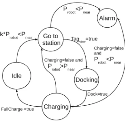
Vinecharger flows according Vinecharger State Machine, which has five states: Idle, Go to Station, Alarm, Docking and Charging. The transition between these states is trigged by the available energy and according a pre-processed charging trajectory and energy map (PCTEM), Fig.3.
3.1 Off Line Path Planning
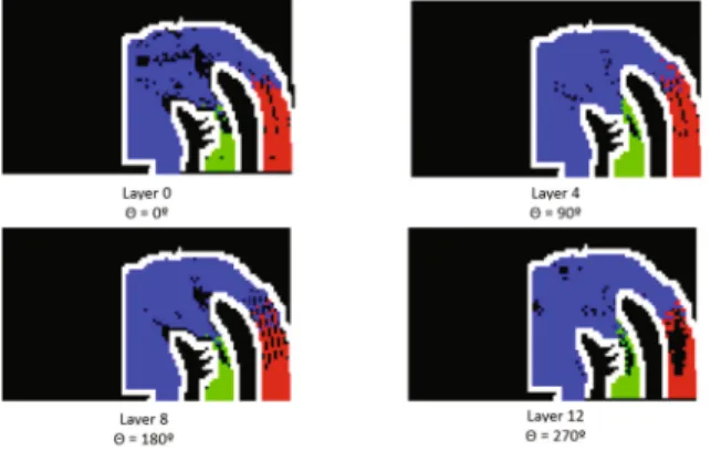
To process the charging trajectory and energy map (PCTEM) represented in Fig.3, we resorted to an A* algorithm developed in [21] that restricts the path to the maximum turning rate allowed by the robot, assuring that the generated path is feasible for the robot. This A* uses a 16 layered occupation grid map, each layer corresponding to a different orientation, spaced by 22.5◦.
Each charging location is located in the center, (a, b), of a parametric circum-ference (x, y) with ar radius and at parameter represented in Eq.1. In Fig.3,
Fig. 2.Vinecharger architecture and state machine
Fig. 3.Preprocessed charging trajectory and energy map.
these charging locations are represented with red cells on the occupation grid map.
x =a+rcos(t), 0≤t≤2π
y =b+rsin(t), 0≤t≤2π (1)
So, the off-line planning method is composed by these three steps: 1. The off line path planning for each cell and each layer:
(a) Plan a path with origin in the actual cell, to a point (x, y) of the circle that delimits the charging zone, consideringr= 0. If the A* doesn’t find a way, we increase the value ofr, and try to plan a new path.
(c) Go trough every cell occupied by the chosen path, saving that trajectory in each cell so that we don’t need to generate a path on every single cell of the map.
3.2 Energetic Cost
The energy consumption between the point i−1 and i is given by the Eq.2, where instead of using the absolute value of the gravitational acceleration, we calculated it’s distribution by the three axis in the world (x, y, z), in a such way that the consumed energy increases when the robot is going up the vineyard, and decreases when the robot it’s going down.
Ei−i,i=m jf
j=1
(µgzj +aj)vj∆t−m
jf
j=1
(µgxj +aj)vj∆t (2)
– m= robot’s mass
– µis the friction coefficient, and g= (gx, gy, gz) is the gravitational
accelera-tion
– ais the robot’s acceleration andv it’s his speed – ∆tis a small time variation chosen for discretization
– j ∈N[0jf] , whenuj
f ≥1 (ujf defined in Eq.5)
The generated path is described by parametric B´ezier curves, defined in the Eqs.3 and 4. The first equation (3) is a linear curve that it’s used to describe the trajectory between two waypoints with the same orientation. The second equation (4) is used to describe the trajectory when there’s an orientation change. So, the velocity and acceleration of the robot can be derived from the B´ezier curves that describe the trajectory.
x(u) = (1−u)xi−1+uxi
y(u) = (1−u)yi−1+uyi
(3)
x(u) = ((1−u)2)x
i−1+ 2u(1−u)xa+u2xi
y(u) = ((1−u)2)y
i−1+ 2u(1−u)ya+u2yi
(4)
– (xi−1, yi−1) and (xi, yi) represent two waypoints
– (xa, ya) is a medium point between the two waypoints, that depends on the
orientation of each one
– uis a parameter that goes from zero to one, and we calculated it so that the robot speed could be constant (Eq.5)
uj+1 =uj+
k2 dx
du 2
|u=uj +
dy du
2 |u=uj
3.3 Docking Controller (B´ezier Curve)
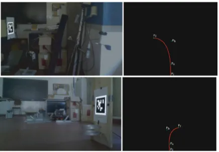
When the robot reaches near to docking station, eventually a visual tag (placed on docking station) will be detected by the Vision Based docking system. When the visual tag is detected the Vinecharger makes the transition from
Gotothestation to Docking state. The tag relative position and orientation is obtained and then the robot’s trajectory is calculated for the docking approach. For that, a cubic B´ezier Curve was used in which the starting point is the posi-tion of the robot at the moment when it saw the tag and the end point is the position of the tag at that every moment. The pointsPi,Pa, Pb andPf of the
B´ezier Curve (BP) are given by the Eq.6. These points are represented on the
right side of Fig.4.
BP = ⎧ ⎪ ⎪ ⎪ ⎪ ⎪ ⎪ ⎪ ⎪ ⎪ ⎪ ⎪ ⎪ ⎪ ⎪ ⎪ ⎪ ⎪ ⎪ ⎪ ⎪ ⎪ ⎪ ⎪ ⎪ ⎪ ⎪ ⎪ ⎪ ⎪ ⎪ ⎨ ⎪ ⎪ ⎪ ⎪ ⎪ ⎪ ⎪ ⎪ ⎪ ⎪ ⎪ ⎪ ⎪ ⎪ ⎪ ⎪ ⎪ ⎪ ⎪ ⎪ ⎪ ⎪ ⎪ ⎪ ⎪ ⎪ ⎪ ⎪ ⎪ ⎪ ⎩
xi =yi=ya= 0
xa =xf×0.30
xf =ztag detector
yf =−xtag detector
mf = (
yf+sin(pitch−π)∗5)−yf (xf+cos(pitch−π)∗5)−xf
ma= 0, ifmf <0 &yf <0
ifmf >0 &yf >0
ma= −1
mf, ifmf <0 &yf >0
ifmf >0 &yf <0
xb =xtarget, ifmtarget= inf
yb=ma×xb−ma×xa+ya, ifmf = inf
xb =ybm−ya
a +xa, ifmf = 0
xb = yb×yf
mf +xf, ifma= 0
yb=ya, ifma= 0
xb =
xa×ma−ya−xf×mf+yf
ma−mf , ifma= inf &mf = inf
&ma×mf = 0
yb=mf×xb−mf×xf+yf, ifmf = inf &ma= 0
(6)
Algorithm1presents the pseudocode with the steps of the docking process.
Algorithm 1. Docking process 1: Get cubic B´ezier Curve points.
2: Transition: global position→relative position.
3: Use a local controller for docking approach.
4
Tests and Results
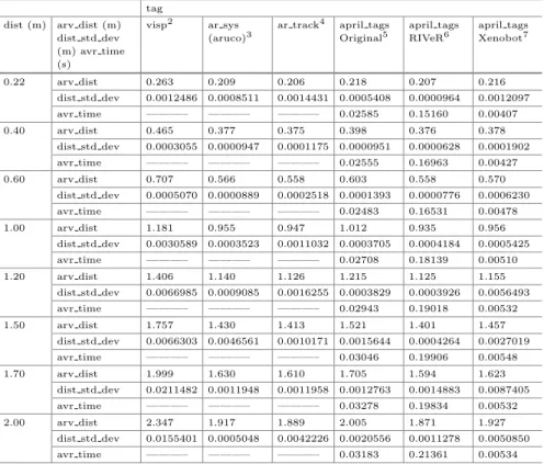
Table 1.Results obtained from tests performed using several tags at various distances.
tag dist (m) arv dist (m)
dist std dev (m) avr time (s)
visp2
ar sys (aruco)3
ar track4
april tags Original5
april tags RIVeR6
april tags Xenobot7
0.22 arv dist 0.263 0.209 0.206 0.218 0.207 0.216
dist std dev 0.0012486 0.0008511 0.0014431 0.0005408 0.0000964 0.0012097
avr time ———– ———– ———– 0.02585 0.15160 0.00407
0.40 arv dist 0.465 0.377 0.375 0.398 0.376 0.378
dist std dev 0.0003055 0.0000947 0.0001175 0.0000951 0.0000628 0.0001902
avr time ———– ———– ———– 0.02555 0.16963 0.00427
0.60 arv dist 0.707 0.566 0.558 0.603 0.558 0.570
dist std dev 0.0005070 0.0000889 0.0002518 0.0001393 0.0000776 0.0006230
avr time ———– ———– ———– 0.02483 0.16531 0.00478
1.00 arv dist 1.181 0.955 0.947 1.012 0.935 0.956
dist std dev 0.0030589 0.0003523 0.0011032 0.0003705 0.0004184 0.0005425
avr time ———– ———– ———– 0.02708 0.18139 0.00510
1.20 arv dist 1.406 1.140 1.126 1.215 1.125 1.155
dist std dev 0.0066985 0.0009085 0.0016255 0.0003829 0.0003926 0.0056493
avr time ———– ———– ———– 0.02943 0.19018 0.00532
1.50 arv dist 1.757 1.430 1.413 1.521 1.401 1.457
dist std dev 0.0066303 0.0046561 0.0010171 0.0015644 0.0004264 0.0027019
avr time ———– ———– ———– 0.03046 0.19906 0.00548
1.70 arv dist 1.999 1.630 1.610 1.705 1.594 1.623
dist std dev 0.0211482 0.0011948 0.0011958 0.0012763 0.0014883 0.0087405
avr time ———– ———– ———– 0.03278 0.19834 0.00532
2.00 arv dist 2.347 1.917 1.889 2.005 1.871 1.927
dist std dev 0.0155401 0.0005048 0.0042226 0.0020556 0.0011278 0.0050850
avr time ———– ———– ———– 0.03183 0.21361 0.00534
4.1 Visual Tags Detector Benchmarking
Six visual tags and detectors were tested in terms of accuracy, robustness, and processing time of various solutions available for detection of artificial landmarks. The table1 summarizes the results of the tests performed using four types of tags, however six implementations were tested: visp,2 ar sys,3 ar track,4 april tags original,5april tags RIVer,6april tags Xenobot.7 This benchmarking was performed in an indoor environment and the HD Web Camera (1280×720 resolution) of the ASUS K750JB notebook with an Intel Quad Core i7-4700HQ (@2.4 GHz) processor, 12 GB of RAM and Ubuntu 14.04 LTS was used.
For each one tested distance was obtained 1000 measurements (avr dist), the standard deviation of these measurements (dist std dev) as well as the average
2 VispAutoTracker implementation:http://wiki.ros.org/visp auto tracker. 3 ArSys implementation:http://wiki.ros.org/ar sys.
4 ArTrackAlvar implementation:http://wiki.ros.org/ar track alvar.
5 AprilTags original implementation:http://people.csail.mit.edu/kaess/apriltags. 6 AprilTags RIVeR-Lab implementation:http://wiki.ros.org/apriltags ros.
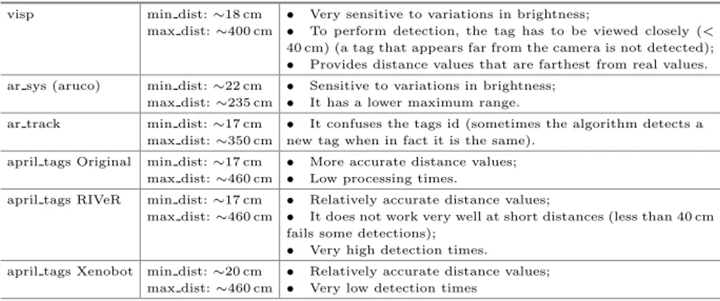
Table 2.Characteristics of the detection algorithms.
visp min dist:∼18 cm max dist:∼400 cm
• Very sensitive to variations in brightness;
• To perform detection, the tag has to be viewed closely (< 40 cm) (a tag that appears far from the camera is not detected);
• Provides distance values that are farthest from real values. ar sys (aruco) min dist:∼22 cm
max dist:∼235 cm
• Sensitive to variations in brightness;
• It has a lower maximum range. ar track min dist:∼17 cm
max dist:∼350 cm
• It confuses the tags id (sometimes the algorithm detects a
new tag when in fact it is the same). april tags Original min dist:∼17 cm
max dist:∼460 cm
• More accurate distance values; • Low processing times.
april tags RIVeR min dist:∼17 cm
max dist:∼460 cm
• Relatively accurate distance values;
• It does not work very well at short distances (less than 40 cm
fails some detections);
• Very high detection times.
april tags Xenobot min dist:∼20 cm
max dist:∼460 cm
• Relatively accurate distance values; • Very low detection times
tag detection time (avr time). The value of thedist is given by the tested algo-rithms and thetimecorresponds to the elapsed time since the detection of the tag until its distance and position are provided. For thevisp,ar sysandar track, the time parameter could not be measured. This procedure was repeated for eight different distances between 22 cm and 200 cm.
Table2shows some characteristics of the detection algorithms that were iden-tified during the tests.
As it is possible to verify through the Tables1 and 2, the best solution is the original implementation ofAprilTags, because it was the one that provided distance values closer to the real and has a very low standard deviation of the measurements. However, this implementation does not provide a ROS node that publishes the information (position and orientation) of the identified tag so that it can be used by other nodes. So two implementations have been tested that pub-lish this information. Of these two implementations the best was theAprilTags Xenobotimplementation because, compared to theAprilTags RIVeR-Lab imple-mentation, the distance values (although a little distant) are closer to the real values and the average processing time is much shorter. In this way theAprilTags Xenobot implementation was chosen for the further development of the system, not because it stands out from the other implementations but because it does not present the problems of the same ones.
4.2 Docking and Off Line Path Planning Test
Fig. 4.Detected tag (left) and Bezier Curve obtained (right).
4.3 Tests and results for energy consumption
Considering the Agrob simulation framework [5] and the next parameters for the Energetic Cost algorithm: m = 1 kg µ= 0.06 g = 9.8 ms−2 v = 1 ms−1 a=
0 ms−2 ∆t = 0.001s C
mass = (0,0,0.4)m. Two paths with different lengths
were tested, one going down and other going up, with the results shown in the Table3. As expected, the energy consumption increases with distance and when going uphill.
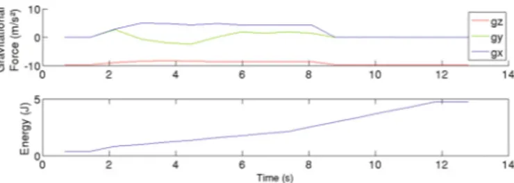
Graphically, Fig.5represents a graphic with the gravitational force imposed by the terrain to the robot, g = (gx, gy, gz), and the energy consumption
expressed in Joules, during a downhill from altitude 12 m to 0 m and a dis-tance of 10 m. In Fig.5, we can observe that in a downhill path the gravitational force ingxtakes positive values, meaning that it’s a force that helps to the robot
movement, being visible an attenuation in the energy consumption. The opposite
Table 3.Energetic consumption
Energy (J) 19 m 9 m
Downhill Uphill Downhill Uphill
1 8.5 12 3.7 4.7
2 8.4 11 3.6 4.9
3 8.48 10.95 3.3 4.8
Fig. 5. Graphical representation of gravitational acceleration and consumed energy during downhill.
Fig. 6.Location of the charging stations
would happen during an uphill, wheregx would take negative values, dragging
back the robot, and consequently, the energy consumption would increase.
4.4 Tests and Results Off-Line PCTEM Processing
To test off-line PCTEM processing, we have considered the occupation map from AGROB simulation framework [5] and three charging stations, Fig.6, identified by numbers: 1, 2 or 3, and color: blue, green or red, respectively. Each station is located in a different altitude, being the station number 1 the one with minimum altitude, and the number 3 the station with maximum altitude.
Fig. 7.Results for the off-line planning
5
Conclusion
The proposed VineRecharge system was developed considering the constrains of a cost-effective robot to carry-out crop monitoring tasks in steep slope vine-yards, and reduces computational power required by the robot even in situation of obstacle avoidance, for example can be easily integrated with Virtual Force Field (VFF) and the Vector Field Histogram (VFH) Methods. Besides, the path planning to the docking station can be immediately obtained from the PCTEM, by using the directional vector stored in each cell of PCTEM. In terms of visual tags, theAprilTags Xenobot implementation was chosen for the further develop-ment of the system, not because it stands out from the other impledevelop-mentations but because it does not present the problems of the same ones. As future work we intend to carry out the tests in a real vineyard step slope scenario.
Acknowledgment. This work is financed by the ERDF – European Regional Devel-opment Fund through the Operational Programme for Competitiveness and Interna-tionalisation - COMPETE 2020 Programme within project “POCI-01-0145-FEDER-006961”, and by National Funds through the FCT – Funda¸cao para a Ciˆencia e a Tecnologia (Portuguese Foundation for Science and Technology) as part of project UID/EEA/50014/2013.
References
1. euRobotics: Strategic research agenda for robotics in Europe Information (2013). http://ec.europa.eu/research/industrial technologies/pdf/robotics-ppp-roadmap en.pdf
2. Bac, C.W., Henten, E.J., Hemming, J., Edan, Y.: “Harvesting robots for high-value crops: state” of-the-art review and challenges ahead. J. Field Robot.31(6), 888–911 (2014)
5. Dos Santos, F.N., et al.: Towards a reliable robot for steep slope vineyards monitoring. J. Intell. Robot. Syst. Article 340 (2016). https://doi.org/10.1007/ s10846-016-0340-5
6. Won, P., Biglarbegian, M., Melek, W.: Development of an effective docking system for modular mobile self-reconfigurable robots using extended kalman filter and particle filter. Robotics4(1), 25–49 (2015)
7. Kim, M., Kim, H.W., Chong, N.Y.: Automated robot docking using direction sens-ing RFID. In: 2007 IEEE International Conference on Robotics and Automation, pp. 4588-4593 (2007)
8. Mintchev, S., et al.: Towards docking for small scale underwater robots. Auton. Robots38(3), 283–299 (2015)
9. Zhu, Y., et al.: A multi-sensory autonomous docking approach for a self-reconfigurable robot without mechanical guidance. Int. J. Adv. Robot. Syst. 11, 10 (2014)
10. Roh, S., Park, J.H., Lee, Y.H., Song, Y.K., Yang, K.W., Choi, M., Kim, H.-S., Lee, H., Choi, H.R.: Flexible docking mechanism with error-compensation capability for auto recharging system of mobile robot. Int. J. Control Autom. Syst.6(5), 731–739 (2008)
11. Acuna, R., Li, Z., Willert, V.: MOMA: Visual Mobile Marker Odometry (2017). arXiv preprintarXiv:1704.02222
12. Briggs, A.J., Scharstein, D., Braziunas, D., Dima, C., Wall, P.: Mobile robot navi-gation using self-similar landmarks. In: 2000 Proceedings of the IEEE International Conference on Robotics and Automation, ICRA 2000, vol. 2, pp. 1428-1434 (2000) 13. Dutta, V.: Mobile robot applied to QR landmark localization based on the keystone effect. In: Mechatronics and Robotics Engineering for Advanced and Intelligent Manufacturing, pp. 45–60 (2017)
14. Yoon, K.J., Jang, G.J., Kim, S.H., Kweon, I.S.: Fast landmark tracking and local-ization algorithm for the mobile robot self-locallocal-ization. In: IFAC Workshop on Mobile Robot Technology, pp. 190–195 (2001)
15. Lo, D., Mendon¸ca, P.R., Hopper, A.: TRIP: A low-cost vision-based location sys-tem for ubiquitous computing. Pers. Ubiquit. Comput.6(3), 206–219 (2002) 16. Zeybek, T., Chang, H.: Delay tolerant network for autonomous robotic vehicle
charging and hazard detection. In: 2014 IEEE/ACIS 13th International Conference on Computer and Information Science (ICIS), pp. 79–85 (2014)
17. Chae, H., Han, K.: Combination of RFID and vision for mobile robot localization. In: Proceedings of the 2005 International Conference on Intelligent Sensors, Sensor Networks and Information Processing Conference, pp. 75–80 (2005)
18. Jang, G., Lee, S., Kweon, I.: Color landmark based self-localization for indoor mobile robots. In: 2002 Proceedings of the IEEE International Conference on Robotics and Automation, ICRA 2002, vol. 1, pp. 1037–1042 (2002)
19. Lin, C.C., Tummala, R.L.: Mobile robot navigation using artificial landmarks. J. Field Robot.14(2), 93–106 (1997)
20. Boley, D.L., Steinmetz, E.S., Sutherland, K.T.: Robot localization from landmarks using recursive total least squares. In: 1996 Proceedings of the IEEE International Conference on Robotics and Automation, vol. 2, pp. 1381-1386 (1996)