A stochastic space-time model for the generation of daily rainfall in the Gaza Strip

Int. J. Climatol.(2011)

Published online in Wiley Online Library (wileyonlinelibrary.com) DOI: 10.1002/joc.2305

A stochastic space-time model for the generation of daily

rainfall in the Gaza Strip

Muamaraldin Mhanna* and Willy Bauwens

Department of Hydrology and Hydraulic Engineering, Vrije Universiteit Brussel, Pleinlaan 2, 1050 Brussels, Belgium

ABSTRACT: An important limitation of commonly used single-site rainfall models is that they are not able to reflect spatial characteristics, while many impact studies demand the accommodation of spatial rainfall correlations. As a result, a number of stochastic models have been developed to produce precipitation simultaneously at multiple sites. One of these models is the Wilks approach [1998.Journal of Hydrology 210: 178 – 191], which was the first method that sufficiently reproduces the main statistics of rainfall at a number of sites. So far, however, the literature does not provide many details about the ‘step by step’ procedure proposed by Wilks. In this paper, the Wilks approach is demonstrated for multi-site, daily rainfall occurrences and amounts in the Gaza Strip. The paper demonstrates a complete methodology taking into account the original Wilks approach and suggests solutions for enhancing the model. The first improvement concerns an analytical calculation of the desired correlations in the random numbers that reproduce the observed correlations between the rainfall occurrence series, through a gamma coefficient. Secondly, the correlations between the rainfall amount series are specified using a rank correlation and then linearly transformed into product-moment correlations to obtain the required correlations in the random numbers. Statistical analyses on the historical and generated rainfall series confirm that the model generally performs well, as it preserves all major characteristics of daily rainfall, as well as spatial characteristics. Major advantages of this model include its simplicity, its increased efficiency, a significant improvement in computational speed and a considerable gain in the effort for the implementation. Copyright_{2011 Royal Meteorological Society}

KEY WORDS multisite rainfall model; Wilks approach; daily rainfall; stochastic process; Markov chain; precipitation; Gaza Strip

Received 30 September 2010; Revised 21 January 2011; Accepted 24 January 2011

1. Introduction

Most agricultural, hydrological, and ecological models require daily rainfall data. However, at many sites such data are often incomplete, too short, or simply unavail-able, which constitutes a serious limitation for these applications. Accordingly, mathematical models, known as stochastic weather generators, have been developed to produce long synthetic weather sequences that are statistically similar to historical records (e.g. Wilks and Wilby, 1999). Numerous approaches for the generation of daily rainfall data at single point are available in the hydrological and climatological literature (e.g. Richard-son, 1981; Srikanthan and McMahon, 1985; Woolhiser, 1992; Sharma and Lall, 1999; Hayhoe, 2000; Wanet al., 2005; Srikanthan et al., 2005; Zheng and Katz, 2008a; Liuet al., 2009). These models are widely used because they are based on a relatively simple stochastic process and are easy to formulate and fast to implement (Wilks, 1999; Mehrotraet al., 2005). Nevertheless, a major lim-itation of widely used single-site rainfall generators is that they are not able to account for spatial charac-teristics: the resulting rainfall time series for different

* Correspondence to: Muamaraldin Mhanna, Department of Hydrology and Hydraulic Engineering, Vrije Universiteit Brussel, Pleinlaan 2, 1050 Brussels, Belgium. E-mail: mmhanna@vub.ac.be

locations are independent of each other, while a strong spatial correlation can often exist in real rainfall data (Wilks, 1999; Qianet al., 2002; Srikanthan and McMa-hon, 2001). Many authors have stressed the importance to account for the spatial correlation of rainfall for flow generation applications, e.g. (Mehrotraet al., 2006; Qian

et al., 2002). In view of scenario analysis, it is there-fore very important to capture the spatial dependence in simultaneous simulations of rainfall sequences at multiple locations.

In order to address the problem of these spatial cor-relations of rainfall, a number of studies have been carried out on the simulation of daily rainfall at a number of sites (e.g. Bras and Rodriguez-Iturbe, 1976; Cox and Isham, 1988; Bardossy and Plate, 1992; Hughes and Guttorp, 1994; Allerup, 1996; Hughes

et al., 1999). However, as discussed in Wilks (1999) and Qian et al. (2002), these approaches are compara-tively complex in both calibration and implementation, and thus their operational application has been lim-ited.

series having realistic spatial correlations. As pointed out by Brissette et al. (2007), the approach represents the first method that adequately reproduces the main statis-tics of precipitation data series at multiple sites. There-fore, this method is of great interest to further improve-ments and it has been used by many researchers (e.g. Qianet al., 2002; Khaliliet al., 2004; Srikanthan, 2005; Mehrotra et al., 2006; Brissette et al., 2007; Thomp-son et al., 2007; Srikanthan and Pegram, 2009). Nev-ertheless, the literature does not provide many more details about the step by step procedure proposed by Wilks. The research carried out by Brissetteet al. (2007) can be considered as the most detailed work done to date.

This study aims to develop a multi-site daily precip-itation generator, based on the approach proposed by Wilks (1998), for the simulation of rainfall occurrences and amounts in the Gaza Strip. The paper attempts to presents a complete methodology based on the original Wilks approach, discusses the associated difficulties and suggests enhancements of the model to circumvent some of these difficulties.

A safe, clean, and adequate water supply is vital to the sustenance of all human beings. Albert Szent-Gyorgyi (Hungarian Biochemist, 1937 Nobel Prize for Medicine) said: “Water is life’s mater and matrix, mother and medium. There is no life without water”. Never has this been truer than it is in the Gaza Strip where around two million Gazans are deprived of access to this essential component of life, and water scarcity represents a real nightmare for people in this area. Rainwater harvesting, now more than ever, became a strategic option to ensure that water demands are met. The rainfall event characteristics for a given region are the most fundamental elements for designing a water harvesting system (Prinz and Singh, 2000). However, the Gaza Strip is generally characterized by very high variability of rainfall in both time and space. Therefore, for catchment scale, the pattern of dry and wet periods, the amounts and the spatial characteristics of rainfall are potentially important, since they directly affect the occurrence and quantity of runoff. Despite this fact, we are not aware of any multi-site application being developed for the study area. Consequently, in order to support the implementation of the rainwater harvesting systems, the stochastic rainfall model is developed mainly

for running a simulation model used to evaluate the performance of large-scale collection systems in the Gaza Strip.

2. Data and study area

The daily precipitation measurements for this study come from eight meteorological stations in the Gaza Strip and cover a period of 33 years (September 1973–September 2006). The data were collected from the Palestinian Meteorology Office in the Ministry of Transport. The locations of the stations are shown in Figure 1. Table I also provides the corresponding annual rainfall and the coefficients of variation.

Generally, the Gaza Strip has a typical semi-arid climate as it is located in the transitional zone between a temperate Mediterranean climate in the west and north, and the arid desert climate of the Sinai Peninsula in the east and south. Therefore, despite the small area of the Gaza Strip (365 km2), the amount of rainfall varies significantly from one location to the next with an average annual rainfall of about 420 mm in the north

Figure 1. Location map of the rainfall stations. This figure is available in colour online at wileyonlinelibrary.com/journal/joc Table I. General information about the selected stations.

Station Name Code Latitude Longitude Annual rainfall (mm) Coefficient of variation (%)

Bait Hanoun Han 31°₃₃′ ₃₄°₃₂′ _{410 38.96}

Bait Lahia Lah 31°₃₄′ ₃₄°₂₈′ _{420 41.05}

Shati Camp Sha 31°₃₂′ ₃₄°₂₈′ _{385 40.12}

Gaza Gaz 31°₃₁′ ₃₄°₂₇′ _{370 38.95}

Nusseirat Nus 31°₂₆′ ₃₄°₂₃′ _{350 41.86}

Deir El Balah Dei 31°₂₅′ ₃₄°₂₁′ _{320 44.04}

Khan Younis Kha 31°₂₁′ ₃₄°₁₉′ _{285 47.45}

(north governorate), to 230 mm in the south (Rafah governorate). Due to the influence of rising altitudes, the yearly rainfall amount increases inland. Most rain falls in the period between mid-October until the end of March. The period from May to September is dry with no rainfall. Precipitation patterns include thunderstorms and rain showers, but only a few days of the wet months are rainy days.

3. The Wilks approach

Wilks (1998) proposed an extension of the well known first-order Markov chain for rainfall occurrences and a mixed exponential distribution for rainfall amounts, to simulate rainfall simultaneously at multiple sites. The approach comprises the use of serially independent and spatially correlated random numbers, which are then employed individually to generate precipitation occur-rence and amount time series at each site. While the original approach of Wilks is applied here, the amounts of rainfall are not modeled by a mixed exponential dis-tribution but by a two-parameter gamma disdis-tribution, as earlier studies have shown that the latter distribution is more suited for the rainfall in the Gaza Strip (Mhanna and Bauwens, 2009). Following Wilks, the rainfall occur-rences are simulated by using a first-order Markov chain. The subsequent paragraphs describe the procedure fol-lowed to generate the spatially correlated random num-bers and their use in the generation of rainfall occurrences and amounts at multiple locations.

3.1. The occurrence of precipitation

For each of the (N) sites and for each of the (M) months in the rainy winter half of the year (October–March), an individual local rainfall occurrence model is fitted, result-ing in a total of N×M models. With the aid of these models, the transition probabilities of the rainfall occur-rence can be specified at each site separately. In order to extend the model for the multi-site generation, the sim-ulation of the rainfall occurrence is forced by serially independent but spatially correlated random numbers. In this way, the spatial correlation is preserved in the gen-erated rainfall series across the network of the stations. The general procedure of estimating the correlations of the random number and the extension of the model is explained in the ensuing paragraphs.

3.1.1. Step 1: Determination of the conditional and unconditional probabilities of rainfall occurrence

The occurrence of precipitation is determined by using the widely used ‘chain-dependent process’ consisting of a first-order two-state Markov process. This model was chosen, in preference to a zero-order, or a second-order Markov model, for its adequacy based on the Bayesian Information Criterion (BIC) (e.g. Schwarz 1978; Katz 1981).

The first-order Markov model involves the assumption that the probability of rain on a certain day is condi-tioned by the wet or dry status of the previous day. Let

Xtrepresent the binary event of ‘precipitation’ or ‘no

pre-cipitation’ occurring on dayt. A wet day is defined as occurring whenever the amount of precipitation exceeds a certain threshold, while dry days are days which are not wet. In this study, a day with total rainfall of 0.1 mm or more is considered a wet day. For each site, k, the process is determined by using the two conditional prob-abilities for the wet-day occurrence pattern:P01(k), the

conditional probability of a wet day (Xt =1) given that

the previous day was dry (Xt−1 =0);P11(k), the

condi-tional probability of a wet day given that the previous day was wet. For each month, these two probabilities need to be determined and used to provide a transition from one month to another. As discussed by Wilks (2006), the parameter estimation procedure consists simply of com-puting the conditional relative frequencies, which yield the maximum likelihood estimators (MLEs). Mathemat-ically, these estimators can be expressed as (e.g. Zheng and Katz, 2008b):

ˆ P01(k)=

n01(k) n01(k)+n00(k)

(1)

ˆ P11(k)=

n11(k) n11(k)+n10(k)

(2)

where, for the site k, n01 is the historical count of wet

days following dry days,n00is the historical count of dry

days followed by dry days, and so on.

The unconditional probability of a wet day,π1, for the

sitek, can be derived as (e.g. Katz and Parlange, 1998)

π1(k)=Pr{Xt(k)=1} =

P01(k)

1+P01(k)−P11(k)

; (3)

and the unconditional probability of a dry day being simply

π0(k)=1−π1(k). (4)

3.1.2. Step 2: Determination of the correlations between the rainfall occurrence series

For each two sites,k andl, the correlations between the rainfall occurrence seriesXt(k) andXt(l) are calculated

ξ(k, l)=Corr[Xt(k), Xt(l)] (5)

Given a network ofNlocations, there areN (N−1)/2 pairwise correlations that should be specified and main-tained in the generated rainfall occurrences. Follow-ing Thompsonet al. (2007) and Srikanthan and Pegram (2009), these correlations are calculated in this study as:

ξ(k, l)= π00(k, l)−π0(k)π0(l)

σ (k)σ (l) (6)

Here σ denotes the standard deviation of the binary series

π0(k) and π1(k) are calculated from Equations (3) and

(4). The joint probability that station pairs are both dry,

π00(k, l), is estimated as:

π00(k, l)= dj oint

n (8)

where dj oint denotes the historical count of station pairs

that are both dry on the same day and n is the number of data values.

3.1.3. Step 3: Definition of the stochastic rainfall occurrence model

The stochastic simulation of the Xt series will, as in

the case for a single site model, be forced by a random number generator that produces uniform random numbers

ut(k). Here, however, a problem arises due to the fact

that the number of multivariate uniform distributions with a particular correlation matrix is infinite (Fackler, 1999). In order to circumvent the problem and to account for the necessary correlations, correlated standard normal variateswt(k)∼N[0, 1] will be used to force the

occurrence process. These standard Gaussian variates will subsequently be transformed to uniform variates ut(k)

through the transformation:

ut(k)=[wt(k)] (9)

where [.] indicates the standard normal cumulative distribution function (CDF).

For the forcing of the occurrence process, the normally distributed random numbers (wt) must preserve the

spatial correlation in the rainfall occurrence series. Let

ω(k, l) indicate the correlation between the standard

normal variates, wt(k) and wt(l), which are generated

from a bivariate normal distribution. The aim then becomes to find the value forω(k, l) leading to rainfall occurrences that exhibit a correlation of ξ0(k, l), the observed value ofξ(k, l). The problem that hereby arises is that a direct computation ofω(k, l)fromξ0(k, l)is not possible. Therefore, these correlations are obtained by constructing empirically-derived curves relating ω(k, l)

andξ(k, l)for all N (N−1)/2 station pairs.

As discussed by Wilks (1998), one finds empirically that there is a monotonic relationship between ω(k, l)

and ξ(k, l) for a given station pair k and l. Different

methods can be used to define this relationship:

• by using a nonlinear root finding algorithm through inverting the relationship between ω(k, l) and ξ(k, l)

(Srikanthan and Pegram, 2006);

• by using a maximum likelihood method (Thompson

et al., 2007);

• by using a hidden covariance model (Srikanthan and Pegram, 2009);

• by using trial and error procedure through assigning different values ofω(k, l)and repeating the procedure till a reasonable value of ξ(k, l), close to ξ0(k, l), is achieved (Mehrotraet al., 2006);

Figure 2. The relationship between the random variates correlation [ω(k, l)] and generated occurrences correlation [ξ(k, l)]. Theξ0(k, l)

andξmax are the observed and maximum values ofξ(k, l), and 0.918 is the correlation that has to be considered for the random numbers. This figure is available in colour online at wileyonlinelibrary.com/journal/joc

• by constructing empirically derived curves for each pair of stations (Wilks, 1998).

Figure 2 illustrates the latter method, which is also used in this study. The curve in Figure 2 is constructed by assuming different values for the correlations between random variates, ω(k, l), and by assessing the resulting correlation between the observed binary series of rain-fall occurrences,ξ(k, l). The observed correlation being known (see step 2), the correlation between random vari-ates can be derived.

In the case of the example, given an observed correla-tion of 0.647, the correlacorrela-tion that has to be considered for the random variates is 0.918. It is also seen on the curve that forcing the rainfall occurrence models for these loca-tions with identical standard random numbers yields the correlationξmax(k, l)=0.857.

The multivariate normal variates can now be generated from (e.g. Fackler, 1999):

wt =U Rt (10)

whereRt represents an independent normal vector andU

is a coefficient matrix such that

UTU =. (11)

Heredenotes the covariance matrix, whose elements are the correlationsω(k, l). Note that because of the unit variances the covariance matrix is also the correlation matrix (Diaset al., 2008).

definite matrix. In case of a non-positive-definite, the matrix should be smoothed. This can be done by modelling the different correlationsω(k, l)as a function of site separation, which accounts for differences in the site locations between the stations, e.g.:

ξ(k, l)=exp(b0+b1|xkl| +b2|λkl| +b3|hkl|)

(12)

Here, xkl is the horizontal distance between the

stationsk andl,λklis the east–west component of the

horizontal separation, andhklis the vertical separation.

Once the covariance matrix is positive-definite, the ele-ments ofUcan be obtained by Cholesky’s decomposition (e.g. Fackler, 1999).

After accounting for the necessary spatial correlations, each set of the resulting serially independent random numbers, wt(k), is then used to generate precipitation

occurrence time series at a particular site k. These numbers are compared to the appropriate conditional probability for a wet-day occurrence pattern [P01(k)and P11(k)], taking into consideration the wet-dry status of

the previous day. This threshold is defined as Critical Probability,Pc, (Wilks, 1998):

Pc(k)=

P01(k) if Xt−1(k)=0

P11(k) if Xt−1(k)=1 (

13)

Then, the following wet day is generated if the random number is adequately small:

Xt(k)=

1 if [wt(k)]≤Pc

0 otherwise (14)

3.2. The amount of precipitation

As already shown for the rainfall occurrence model, the rainfall amount is forced by serially independent and spatially correlated random numbers that must preserve the spatial correlation in the rainfall amount series. The general procedure of generating rainfall amount series at a number of sites is explained in the following paragraphs.

3.2.1. Step 1: Determination of the model parameters

The rainfall amounts on wet days are generated by using a 2-parameter Gamma distribution whose probability density function for sitek is defined as (e.g. Katz, 1977):

f[rt(k)]=

[rt(k)/β(k))]α(k)−1exp[−r(k)/β(k)]

β(k)Ŵ[α(k)] ;

x, α, β >0; (15)

wherert(k)is the non-zero precipitation amounts,αand

βdenote the parameters of shape and scale, respectively, andŴ(α)is the Gamma function evaluated atα.

The parameters of the model are calculated, for each site k and for each month in the rainy winter half of the year, by using the method of maximum likelihood

through the Thom approach (Thom, 1958). The maximum likelihood estimator for the shape parameter is given by

ˆ

α(k)= 1+

1+4A(k)/3

4A(k) , (16)

and for the scale parameter is calculated as

ˆ

β(k)= Y (k)

ˆ

α(k). (17)

Here Y denotes the mean daily rainfall (mm) for the month, considering only wet days, andAis the difference between the logs of the arithmetic and geometric means.

3.2.2. Step 2: Determination of the correlation between the rainfall amount series

For two sites,kandl, the correlations between the rainfall amount seriesYt(k)andYt(l)are calculated:

η(k, l)=Corr[Yt(k), Yt(l)] (18)

In this study, these correlations are calculated using the Pearson product-moment correlation. As the Gamma model attempts to generate rainfall amounts on wet days for site k, the correlations between the rainfall amount series for two sites (k andl) is calculated by taking into consideration that both sites are wet.

3.2.3. Step 3: Definition of the stochastic rainfall amount model

The spatial correlation in the daily rainfall amounts is preserved by using a vector of correlated uniform variates

vt. As detailed previously for the rainfall occurrence

model, it is convenient to obtain the elements of this vector from a corresponding realization of correlated standard normal variateszt(k) as vt(k)=[zt(k)].

The vectorzt can be drawn from a multivariate normal

distribution with mean 0 and covariance matrix [], whose elements are:

ζ (k, l)=Corr[zt(k), zt(l)] (19)

Together with the corresponding correlation ω(k, l)

and the Markov chain and Gamma parameters for the stations k and l, a particular ζ (k, l) yields a unique correlationη(k, l)between the synthetic rainfall amounts for the two sites.

Similar to the case for finding the binary , a direct computation of is not feasible since the zt are not

observed. The correlations in Equation (19) are thus estimated by applying an analogous procedure to the one used in the rainfall occurrence model.

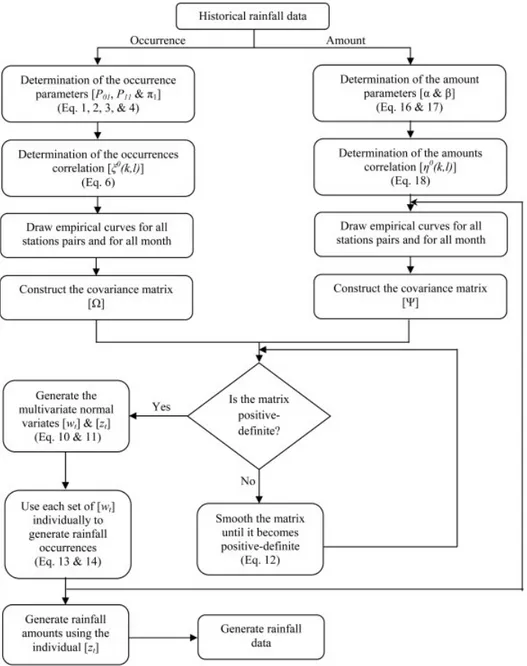
Figure 3. General steps of the original Wilks approach applied in this study for the generation of multi-site precipitation data.

The correlated multivariate normal variates are ob-tained from independent normal variates through a similar transformation, employing Equations (10) and (11).

Overall, the steps required for the simulation of pre-cipitation occurrences and amounts at a number of sites are summarized in Figure 3.

4. The modified Wilks approach

The original approach of Wilks involves constructing N×(N−1)/2 curves of the type shown in Figure 2 for each month (and for all station pairs), in order to generate series with the same correlation as the observed ones. However, such construction may result in the non-positive-definiteness of the covariance matrices. Wilks overcomes this problem by modelling the pair-wise correlations of the random numbers as a function of site separation (Equation (12)). However, the approach

is not efficient and requires a significant amount of time.

In what follows, we suggest improvements of the Wilks approach by two analytical solutions for the calculation of the desired correlations in the random numbers for the simulation of the rainfall occurrences and amounts. Moreover, the propped improvements also imply the use of a pragmatic and simpler method to ensure positive-definiteness of the resulting covariance matrices.

4.1. The occurrence of precipitation

The dependence measure in Equation (6), which is used to calculate the correlations between the rainfall occur-rence series, depends on the joint probability that station pairs are both dry,π00(k, l)and on the marginal

probabil-ities π0(k) and π0(l). However, during the construction

Figure 4. The relationship between the random variates correlation [ω(k, l)] and the marginal (π0) and joint (π00) probabilities. This figure is available in colour online at wileyonlinelibrary.com/journal/joc

numbers, ω(k, l), does not have any significant impact on the marginal probabilities. In other words, by assum-ing different values for the correlations between random variates, theπ0(k)and π0(l) remain constant during the

process, whereasπ00(k, l)increases gradually asω(k, l)

increases (Figure 4). It is also seen on the curve that the correlation that has to be considered for the random variates, in order to replicate the observed correlation, is practically equal to the needed correlation to repro-duce the π00(k, l). So, by using an appropriate measure

of dependence that relies only on the joint probability, the needed correlations of random numbers can be calculated analytically.

The gamma coefficient proposed by Goodman and Kruskal (1954) is one of the most useful measures of association that can be used for this purpose. In their investigation of dependence measures for binary data, Tajar et al. (2001) tested seven measures: six of them based on concordance and the other one being the odds ratio. They concluded that the gamma coefficient, in additional to the odds ratio, depends only on the joint probability and not on the marginal probabilities. The basic idea in this approach is to assume that the needed correlations of random numbers are equal to the gamma correlations between the rainfall occurrence series [γ (k, l)=w(k, l)].

The gamma coefficient is calculated as (Rousson, 2007):

γ (k, l)= ϕ(k, l)−1

ϕ(k, l)+1, (20)

whereϕ is odds-ratio and is calculated as

ϕ(k, l)= π00(k, l)π11(k, l) π10(k, l)π01(k, l)

(21)

Hereπ00(k, l)denotes the joint probability that station

pairs are both dry, π11(k, l) is the joint probability that

station pairs are both wet, and so on. 4.2. The amount of precipitation

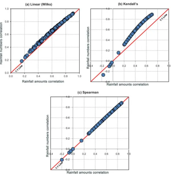
As mentioned earlier, the stochastic simulation is forced by a random number generator that produces correlated normal variates and then transforms them each indi-vidually to obtain uniform marginal distributions. Such non-linear transformation, however, will typically have an influence on the dependence between the random nor-mal variables. This is due to the fact that the Pearson product–moment (linear) correlation is not invariant to transformations of the underlying marginal distribution (Fackler, 1991). Therefore, the linear correlation will not be captured after the transformation if the original normal variates are linearly correlated. The most conve-nient solution to this problem is to use other measures of dependence that are preserved under any monotonic transformations (Fackler, 1991). One of those measures is the rank correlation (also called fractile correlation) which is invariant with respect to strictly increasing trans-formations of the variables involved (e.g. Ghosh and Henderson, 2003; Phoon et al., 2004). The key to this method is to specify the correlations between rainfall series using a fractile correlation and then linearly con-vert them into the product–moment correlation to obtain the needed correlations of random numbers. As a result, the linear correlation between the uniforms obtained from transforming the normal variates will result in a synthetic rainfall series that exhibits the rank correlation between rainfall amounts.

There are two common measures of rank correlation, being the Spearman rank correlation ρ(k, l) and the Kendall’s statistic τ (k, l). The corresponding binomial correlationζ (k, l), the correlations between the standard normal variates, zt(k) and zt(l), can be obtained via

the following relationships between these measures and the product–moment correlation (e.g. Kruskal., 1958; O’Brien and Griffiths, 1965):

ζ (k, l)=sin

πτ (k, l)

2

(22)

ζ (k, l)=2 sin

πρ(k, l)

6

(23)

Figure 5. The observed amounts correlationversus the needed random numbers correlation obtained by (a) Wilks approach, (b) Kendall’s, and (c) Spearman. This figure is available in colour online at wileyonlinelibrary.com/journal/joc

The transformation may result in a non-positive defi-nite matrix, but this is unlikely to occur often in practice since the function in Equation (23) is so close to an iden-tity mapping on [−1, 1] (e.g. Fackler, 1999). However, as discussed in Phoon et al. (2004), a plausible method to overcome this problem is to set the negative eigenval-ues to zero. Brissetteet al. (2007) have applied a similar procedure, as proposed by Rebonato and J¨ackel (2000), to ensure the construction of a valid correlation matrix. Their procedure comprises the diagonalisation and the replacements of all negative eigenvalues with a small positive value, but whereby the correlation matrix is nor-malized using a standard equation. For a detailed dis-cussion, considering the problem of non-positive-defined matrices, readers are referred to Rebonato and J¨ackel (2000).

The required steps for the modified Wilks ap-proach are summarized in Figure 6. In general, this methodology reduces the amount of work presented in Figure 3, resulting in an improvement in the computa-tional speed.

5. Model performance evaluation

The goal of rainfall generators is to produce synthetic rainfall data which are statistically similar to the observed ones. Subsequently, both observed and generated rainfall series are subjected to a standard exploratory data anal-ysis to describe the performance of the daily generation model using a set of statistical parameters. The original Wilks approach and the modified approach have fitted the same stochastic process to produce the precipitation occurrences and amounts at a number of sites. Conse-quently, the main comparison between the model using the original approach to parameter fitting and the model using the modified approach will be based on the abil-ity of the model to preserve spatial characteristics of the historical rainfall series.

The following statistics are used to evaluate the repro-duction of the various characteristics of the processes of rainfall occurrences and amounts:

• the mean number of wet days per month

Figure 6. General steps of the modified Wilks approach for the generation of multi-site precipitation data.

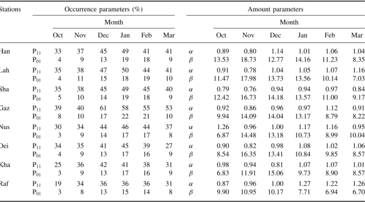
Table II. Monthly values of the parameters needed for precipitation occurrence and amount.

Stations Occurrence parameters (%) Amount parameters

Month Month

Oct Nov Dec Jan Feb Mar Oct Nov Dec Jan Feb Mar

Han P11 33 37 45 49 41 41 α 0.89 0.80 1.14 1.01 1.06 1.04

P01 4 9 13 19 18 9 β 13.53 18.73 12.77 14.16 11.23 8.35

Lah P11 35 38 47 50 44 41 α 0.91 0.78 1.04 1.05 1.07 1.16

P01 4 11 15 18 19 10 β 11.47 17.98 13.73 13.56 10.14 7.03

Sha P11 35 38 45 49 45 40 α 0.79 0.76 0.94 0.94 0.97 0.84

P01 5 10 14 19 18 9 β 12.42 16.73 14.18 13.57 11.00 9.17

Gaz P11 39 40 61 58 55 53 α 0.92 0.86 0.96 0.97 1.12 0.91

P01 8 10 17 22 21 10 β 9.94 14.09 14.04 13.17 8.79 8.22

Nus P11 30 34 44 46 44 37 α 1.26 0.96 1.00 1.17 1.16 0.95

P01 3 9 14 17 17 8 β 6.87 14.48 13.18 10.73 8.99 10.04

Dei P11 34 35 41 45 39 27 α 0.90 0.82 0.98 1.08 1.02 1.06

P01 4 9 13 17 16 9 β 8.54 16.35 13.41 10.84 9.85 8.57

Kha P11 25 36 42 41 38 31 α 0.98 0.94 0.81 1.07 1.07 1.01

P01 3 9 13 17 16 9 β 6.83 11.91 15.06 9.73 8.90 8.57

Raf P11 19 34 36 36 36 31 α 0.87 0.96 1.00 1.27 1.22 1.26

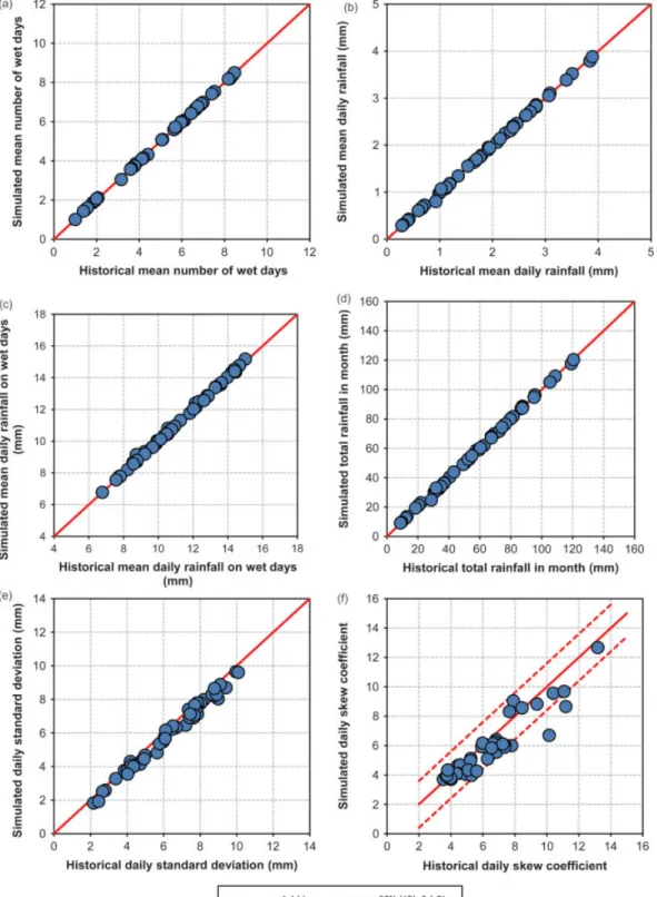
Figure 7. A comparison of historical and generated rainfall statistics, for all stations and all months. (a) Mean number of wet days; (b) mean rainfall; (c) mean rainfall on wet days; (d) total rainfall; (e) standard deviation; (f) skew coefficient. The 95% UCL and LCL are the upper and

lower confidence levels= ±1.96×standard error (0.812). This figure is available in colour online at wileyonlinelibrary.com/journal/joc

• the mean daily rainfall amount on wet days

• the total rainfall amount in a month

• the standard deviation of the daily rainfall amount in a month

• the skew coefficient of the daily rainfall amount in a month

• the cumulative relative frequencies of the daily rainfall depths

The following statistics are used to evaluate the repro-duction of the spatial characteristics and as a comparison between the two approaches:

• the joint probabilities that station pairs are both wet (π11)

Figure 8. Cumulative relative frequencies of the historical and generated daily rainfall depths during the winter half of the year. This figure is available in colour online at wileyonlinelibrary.com/journal/joc

Figure 10. Cross-correlations between the rainfall occurrences, for all station pairs and months. The dashed lines indicate the 95% upper confidence level (UCL) and the 95% lower confidence level (LCL). This figure is available in colour online at wileyonlinelibrary.com/journal/joc

• the cross-correlations of binary wet/dry occurrences between stations

• the cross-correlations of daily amounts (each pair wet) between stations

6. Results and discussion

6.1. Precipitation occurrence and amount

The transition probabilities used by the model to gen-erate daily precipitation occurrences, and the parameters employed to generate daily precipitation amounts with the use of the Gamma distribution are given in Table II. The various daily statistics derived from generated and historical rainfalls are compared in Figures 7 and 8.

For each month of the winter half of the year, the gen-erated and observed mean number of wet days, mean daily rainfall, mean daily rainfall on wet days, the total rainfall per month, the daily standard deviation, and the daily skew coefficient are plotted in Figure 7. The results show that the occurrence model was successful in repro-ducing the mean number of wet days at the eight stations. There was no significant difference between the observed and generated numbers of wet days. The generator model was also successful in producing the mean daily pre-cipitation and the quality of data was satisfactory for all stations. In addition, the model preserves the mean daily precipitation on wet days and the total precipitation per month adequately. The daily standard deviation was well reproduced by the model. The daily skew coefficient was generally considered to be reasonably preserved by the model. Nearly all points, except two, lie within the 95% confidence level of±1.96×standard error (0.812), which confirms that the synthetic values do not differ much from the observed ones.

Figure 8 shows the cumulative relative frequencies of daily rainfall depths during the winter half of the year, simulated by the weather generator, compared with

the observed ones. The results show that the Gamma distribution model can reproduce with high performance the properties of the distributions of daily precipitation amounts.

Overall, the performance of the model is generally considered to be satisfactory for all stations, as the synthetic daily precipitation series generated from the weather generator keep all the important characteristics of the observed series.

6.2. Spatial characteristics

Figure 9 compares the joint probabilities of the observed and generated daily series for all station pairs and all months, for the case where both sites are wet (left side), and for the case that both sites are dry (right side). In Figure 9, each dot corresponds to a given station and a given month of the year. The statistics for the simulated values are based on a simulation of 3000 years. Basing on the figure, it is evident that the full joint distribution of simultaneous precipitation occurrence across the network of the eight stations is well represented by the model for the two approaches for parameter fitting.

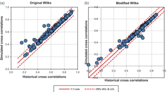
The cross-correlations between the rainfall occurrences at different sites are presented in Figure 10. There is a little distinction between the performances of the model using the original Wilks approach (left side) and the modified approach (right side) with respect to preserving this statistic. Apparently, the model performs quite well for both approaches: most points are positioned within the 95% confidence level of+1.96×standard error (0.045) for the upper level (UCL), and −1.96×0.045 for the lower level (LCL).

Figure 11. Cross-correlations between the rainfall amounts, for all station pairs and months. The dashed lines indicate the 95% upper confidence level (UCL) and the 95% lower confidence level (LCL). This figure is available in colour online at wileyonlinelibrary.com/journal/joc

Figure 12. Mean (a), standard deviation (b), and skew coefficient (c) of the average daily rainfall over the Gaza Strip We have provided “model for generation of rainfall in the gaza strip” as the running head. It will appear on the top of the third page and all the recto pages of the article.

Pls confirm whether this is appropriate. This figure is available in colour online at wileyonlinelibrary.com/journal/joc

the synthetic and observed correlations of the rainfall amounts do not differ much.

Furthermore, as an application, the generated rainfall series of the eight stations are integrated into one series, representing the average rainfall over the Gaza Strip. A comparison between the historical data and the results of the simulations with the model, using the modified Wilks approach to parameter fitting, shows that the statistics are well captured by the model (Figure 12).

Overall, the spatial characteristics of the historical rainfall series seem to be reasonably captured by the model for both approaches.

7. Conclusions

of rainfall occurrences and amounts in the Gaza Strip. A first-order two-state Markov chain is used to determine the occurrence of rainfall. The rainfall amounts on wet days are generated by using the two-parameter Gamma distribution. Parameters of the rainfall model are estimated, for every month in the rainy winter half of the year (October–March), from observed precipitation data by using the method of maximum likelihood.

The paper presents a complete methodology taking into account the original Wilks approach and suggests solutions for enhancing the practical development of the model. The first improvement concerns an analytical cal-culation of the desired correlations in the random num-bers that reproduce the observed correlations between the rainfall occurrence series, through a gamma coefficient. Secondly, the correlations between the rainfall amount series are specified using a rank correlation and then linearly transformed into product-moment correlations to obtain the required correlations in the random num-bers. In the original Wilks approach, this was achieved by constructing all empirically derived curves for each pair of stations and for every monthly period, which may however result in non-positive-definiteness prob-lems. The latter problem is solved in this study by setting the negative eigenvalues to zero or to a small positive value. In Wilks (1998), the problem of a non-positive def-inite correlation matrix was overcome by modeling the pair-wise correlations of the random numbers as a func-tion of site separafunc-tion, which is not efficient and requires a significant amount of time.

Statistical analyses on the historical and synthetic rain-fall series show that the model generally performs well as it preserves all the important characteristics of daily rainfall occurrences and amounts, as well as the spatial characteristics. This superior performance is consistent with the order of the Markov model and the gamma dis-tribution used in this study. It would be interesting to investigate if the proposed fitting algorithms would work as well with higher (or ‘hybrid-‘) order Markov chains and with distributions for nonzero amounts other than the gamma distribution. Overall, major advantages of the model include its simplicity, its increased efficiency, a significant improvement in computational speed and a considerable gain in the effort for the implementation.

References

Allerup P. 1996. Rainfall generator with spatial and temporal char-acteristics. Atmospheric Research 42: 89–97, DOI:10.1016/0169-8095(95)00055-0.

Bardossy A, Plate E. 1992. Space–time model for daily rainfall using atmospheric circulation patterns. Water Resources Research 28: 1247–1260.

Bras R, Rodriguez-Iturbe I. 1976. Rainfall generation: a nonstationary time varying multi-dimensional model. Water Resources Research 12: 450–456, DOI:10.1029/WR012i003p00450.

Brissette FP, Khalili M, Leconte R. 2007. Efficient stochastic generation of multi-site synthetic precipitation data. Journal of Hydrology345: 121–133, DOI:10.1016/j.jhydrol.2007.06.035. Cox DR, Isham V. 1988. A simple spatial-temporal model of rainfall.

Proceedings of the Royal Society of London, Series A415: 317–328. Dias CTDS, Samaranayaka A, Manly B. 2008. On the use of correlated beta random variables with animal population modelling.Ecological Modelling215: 293–300.

Fackler PL. 1991. Modeling Interdependence: an Approach to Simulation and Elicitation. American Journal of Agricultural Economics73: 1091–1097, DOI:10.2307/1242437.

Fackler PL. 1999. Generating correlated multidimensional variates. Working paper, available at http://www4.ncsu.edu/∼pfackler/. Ghosh S, Henderson SG. 2003. Behavior of the NORTA method for

correlated random vector generation as the dimension increases.

ACM Transactions on Modeling and Computer Simulation13: 1–19. Goodman LA, Kruskal WH. 1954. Measures of Association for Cross Classifications.Journal of the American Statistical Association 49: 732–764.

Hayhoe HN. 2000. Improvements of stochastic weather data generators for diverse climates.Climate Research14: 75–87.

Hughes JP, Guttorp P. 1994. Incorporating spatial dependence and atmospheric data in a model of precipitation. Journal of Applied Meteorology33: 1503–1515.

Hughes JP, Guttorp P, Charles S. 1999. A nonhomogeneous hidden Markov model for precipitation occurrence. Journal of the Royal Statistical Society (Series C): Applied Statistics 48: 15–30, DOI:10.1111/1467-9876.00136.

Katz RW. 1977. Precipitation as a chain-dependent process.Journal of Applied Meteorology16: 671–676.

Katz RW. 1981. One some criteria for estimating the order of a Markov chain.Technometrics23: 243–249, DOI:10.2307/1267787. Katz RW, Parlange MB. 1998. Overdispersion phenomenon in

stochastic modeling of precipitation. Journal of Climate 11: 591–601.

Khalili M, Leconte R, Brissette F. 2004. Multisite generation of a daily stochastic precipitation to evaluate the effects of the climatic changes on the Chaˆateauguay River basin hydrology. American Geophysical Union Joint Assembly, May 17–21, Montr´eal, Canada.

Kruskal W. 1958. Ordinal measures of association. Journal of the American Statistical Association53: 814–61.

Liu J, Williams JR, Wang X, Yang H. 2009. Using MODAWEC to generate daily weather data for the EPIC model.Environmental Mod-elling & Software24: 655–664, DOI:10.1016/j.envsoft.2008.10.008. Mehrotra R, Srikanthan R, Sharma A. 2005. Comparison of three approaches for stochastic simulation of multi-site precipitation occurrence. In: Twenty-ninth Hydrology and Water Resources Symposium, Engineers Australia: Canberra, Australia.

Mehrotra R, Srikanthan R, Sharma A. 2006. A comparison of three stochastic multi-site precipitation occurrence generators.Journal of Hydrology331: 280–292, DOI:10.1016/j.jhydrol.2006.05.016. Mhanna M, Bauwens W. 2009. Assessment of a Single-site

Daily Rainfall Generator in the Middle East. In Proc 2nd International Conference on Environmental and Computer Science, Bob Werner (ed.), IEEE Computer Society: California; 14–18, DOI:10.1109/ICECS.2009.19.

O’Brien JJ, Griffiths JF. 1965. The Rank Correlation Coefficient as an Indicator of the Product-Moment Correlation Coefficient for Small Samples (10–100). Journal of Geophysical Research 70: 1995–1998.

Phoon KK, Quek ST, Huang H. 2004. Simulation of non-Gaussian processes using fractile correlation. Probabilistic Engineering Mechanics19: 287–292, DOI:10.1016/j.probengmech.2003.09.001. Prinz D, Singh AK. 2000.Technological Potential for Improvements of Water Harvesting. World Commission on Dams: Cape Town, South Africa.

Qian B, Corte-Real J, Xu H. 2002. Multisite stochastic weather models for impact studies.International Journal of Climatology22: 1377–1397, DOI:10.1002/joc.808.

Rebonato R, J¨ackel P. 2000. The most general methodology to create a valid correlation matrix for risk management and option pricing purposes.Journal of Risk2: 17–27.

Richardson CW. 1981. Stochastic simulation of daily precipitation, temperature, and solar radiation. Water Resources Research 17: 182–190, DOI:10.1029/WR017i001p00182.

Rousson V. 2007. The gamma coefficient revisited. Statistics and Probability Letters77: 1696–1704, DOI:10.1016/j.spl.2007.04.009. Schwarz G. 1978. Estimating the dimension of a model.Annals of

Statistics6: 461–464, DOI:10.2307/2958889.

Sharma A, Lall U. 1999. A nonparametric approach for daily rainfall simulation.Mathematics and Computers in Simulation48: 361–371, DOI:10.1016/S0378-4754(99)00016-6.

Srikanthan R, McMahon TA. 1985. Stochastic generation of rainfall and evaporation data. Water Resources Council: Canberra, Technical Paper; 84.

Srikanthan R, McMahon TA. 2001. Stochastic generation of annual, monthly and daily climate data: a review. Hydrology and Earth System Sciences5: 653–670, DOI:10.5194/hess-5-653-2001. Srikanthan R, Pegram GGS. 2006. Stochastic generation of

multi-site rainfall occurrences. World Scientific Publishing Company. Advances in Geosciences:Hydrological Science6: 1–10.

Srikanthan R, Pegram GGS. 2009. A nested multisite daily rainfall stochastic generation model. Journal of Hydrology371: 142–153, DOI:10.1016/j.jhydrol.2009.03.025.

Srikanthan R, Harrold TI, Sharma A, McMahon TA. 2005. Compari-son of two approaches for generation of daily rainfall data. Stochas-tic Environmental Research and Risk Assessment 19: 215–226, DOI:10.1007/s00477-004-0226-0.

Tajar A, Denuit M, Lambert P. 2001. Copula-type representation for random couples with Bernoulli margins. Discussion Paper 01–18, Institut de Statistique, Universit´e catholique de Louvain, Louvain-la-Neuve, Belgium.

Thom HCS. 1958. A note on the gamma distribution.Monthly Weather Review86: 117–122.

Thompson CS, Thomson PJ, Zheng X. 2007. Fitting a multisite daily rainfall model to New Zealand data. Journal of Hydrology 340: 25–39, DOI:10.1016/j.jhydrol.2007.03.020.

Wan H, Zhang X, Barrow EM. 2005. Stochastic Modelling of Daily Precipitation for Canada.Atmosphere Ocean43: 23–32.

Wilks DS. 1998. Multisite generalization of a daily stochastic precipitation generation model.Journal of Hydrology210: 178–191, DOI:10.1016/S0022-1694(98)00186-3.

Wilks DS. 1999. Simultaneous stochastic simulation of daily precipitation, temperature and solar radiation at multiple sites in complex terrain.Agricultural and Forest Meteorology 96: 85–101, DOI:10.1016/S0168-1923(99)00037-4.

Wilks DS. 2006. Statistical methods in the atmospheric sciences. Academic Press: San Diego.

Wilks DS, Wilby RL. 1999. The weather generation game: a review of stochastic weather models.Progress in Physical Geography 23: 329–357, DOI:10.1177/030913339902300302.

Woolhiser DA. 1992. Modelling daily precipitation – progress and problems. In Statistics in the environmental and earth sciences, Walden AT, Guttorp P (Eds), Edward Arnold: London; 71–89. Zheng X, Katz RW. 2008a. Mixture model of generalized

chain-dependent processes and its application to simulation of interannual variability of daily rainfall. Journal of Hydrology 349: 191–199, DOI:10.1016/j.jhydrol.2007.10.061.