THE IMPACT OF SURFACE HEAT FLUXES ON THE SIMULATION OF THE BRAZIL CURRENT

(1)

THE IMPACT OF SURFACE HEAT FLUXES ON THE SIMULATION OF THE BRAZIL CURRENT

Vladimir Santos da Costa and Afonso de Moraes Paiva

ABSTRACT.The impact of different formulations of surface heat fluxes (no fluxes, climatological fluxes, restoring of SST towards climatology, climatological fluxes plus SST restoring, and model-computed fluxes via bulk formulas) on the modeling of the Brazil Current is investigated in numerical simulations performed with the Regional Ocean Model (ROMS). While mechanical forcing may be dominant, it is shown that correct upper ocean currents and thermal structure can only be obtained when heat fluxes are implemented, even in regions of strong horizontal advection, and that some form of feedback of the ocean state upon the fluxes is also a necessary condition. This results are of particular importance for ocean modeling developed having operational oceanography in view.

Keywords: Brazil Current, surface heat flux, numerical modeling.

RESUMO.O impacto de diferentes formulações dos fluxos de calor em superf´ıcie (sem fluxos, fluxos climatológicos, relaxamento de TSM para climatologia, fluxos climatológicos mais relaxamento de TSM e fluxos calculados pelo modelo com “bulk formulas”) sobre a modelagem da Corrente do Brasil é investigado em simulações numéricas com o Regional Ocean Model (ROMS). Apesar da forçante mecânica ser dominante, mostra-se que uma correta representação de correntes e da estrutura térmica nas camadas superiores do oceano somente são poss´ıveis quando fluxos de calor são implementados e que algum tipo de retroalimentação da TSM sobre os fluxos é também necessária. Estes resultados são particularmente importantes na modelagem voltada para a oceanografia operacional.

Palavras-chave: Corrente do Brasil, fluxos superficial de calor, modelagem num´erica.

Programa de Engenharia Oceânica – COPPE/UFRJ, Av. Horácio Macedo, 2030, Bloco C, sala 203, Centro de Tecnologia, Cidade Universitária, Ilha do Fundão, Cx. Postal 68.508, Rio de Janeiro, RJ, Brazil. Phone: +55(21) 2562-8755 – E-mails: vladimir@peno.coppe.ufrj.br; mpaiva@peno.coppe.ufrj.br

(2)

“main” — 2014/1/3 — 18:13 — page 308 — #2

308

THE IMPACT OF SURFACE HEAT FLUXES ON THE SIMULATION OF THE BRAZIL CURRENT INTRODUCTION

The oceanic circulation off southeast Brazil is complex and highly dynamic. In the slope region, at the surface and down to about 450 m, the Brazil Current (hereafter BC) transports South Atlantic Central Waters and Tropical Water (SACW and TW, respectively) poleward (Stramma & England, 1999; Silveira et al., 2000). At in-termediate levels, underlying the BC until approximately 1500 m, the water moves equatorward in a well defined flow that transports primarily Antarctic Intermediate Water (M¨uller et al., 1998; Sil-veira et al., 2004). This current system, which has been labeled as Brazil Current – Intermediate Current (BC-ICC) System, is baro-clinically unstable (Silveira et al., 2008; Fernandes et al., 2009, Mano et al., 2009) and generates several eddies at some pref-erential locations that may eventually pinch off from the current. Over the adjacent and relatively thin continental shelf, a localized but intense upwelling brings SACW to the surface, and SST can reach values as low as 15C (Moreira da Silva & Mendonc¸a, 1977; Miranda, 1985). The interaction between the upwelled waters and the BC is not yet well characterized, and is the subject of ongoing research. Its signature, however, is clearly depicted from ocean color remote sensing as the high productive coastal waters are captured by the current and by its meanders and eddies.

The BC flow and its mesoscale variability, in particular in the southeast region of Brazil, are the focus of the ongoing REMO project (Brazilian Network for Ocean modeling and observation), which aims for the configuration of an operational forecasting sys-tem for Brazilian oceanic and coastal waters (see companion pa-pers in this same issue for details). Preliminary efforts, and also previous numerical studies presented in the literature on the BC dynamics have addressed the issues of current intrinsic variabil-ity (Calado et al., 2006; Fernandes et al., 2009) and of mechani-cal lomechani-cal wind forcing (Rodrigues & Lorenzzetti, 2001; Castel˜ao & Barth, 2006; Calado et al., 2010). So far, not much attention has been paid to the impacts that heat and mass fluxes at the ocean-atmosphere interface may have upon this system. Although we do not claim that such fluxes represent a dominant aspect of the cur-rent dynamics, we intend to show in the present paper that a care-ful consideration of their formulation and impacts, in particular of the heat fluxes, is essential for a correct simulation of important features of this system.

The heat equation can be expressed for a surface layer of depth 1z as:

dT

dt = ρQc_pnet1z + K∇

2_{T + Rad} ₍₁₎ where_{d/dt is the total derivative, T is the water temperature,} ρ is the water density,c_pis the specific heat at constant

pres-sure, and the third term is the turbulent diffusion of heat. _Rad accounts for the divergence of penetrating incoming solar radia-tion, and its specific formulation is of no particular interest here. We will be primarily concerned with_Q_net, which represents the sum of latent (_Q_l)and sensible (Q_s)heat fluxes plus long wave radiation (_Q_b)at the surface. There are several ways to formulate the net surface heat fluxes in ocean models, and it can be shown (see Paiva & Chassignet, 2001 for a review) that they can all be represented by the general form:

Qnet= Q(T1)+ λ(T2− T ) (2) Depending on the choices for λ (a relaxation coefficient),_T₁ and_T₂(sea surface temperatures) , the model temperatures (_{T )} can be forced by prescribed climatological fluxes, or by model fluxes computed through bulk formulas or through a relaxation of model temperatures to climatological SST or through a combi-nation of prescribed fluxes plus a restoring to climatological SST (see methodology section for details). Forcing ocean models with climatological heat fluxes is generally avoided since this approach leads to long term trends and do not take into account the model state. Pure relaxation to climatological SST, on the one hand, is easy to implement and prevents the model solution from drifting apart too much from a mean or reference state. On the other hand, however, the correct answer (_{T equals to observed SST) can only} be obtained for wrong (null) fluxes (Killworth et al., 2000; Chu et al., 1998). Computing the fluxes during a model run via bulk formulas, using model sea surface temperature and atmospheric variables, may seem at a first glance as a more complete approach that takes the ocean feedback upon the fluxes in a more appro-priate way. However, as discussed by Seager et al. (1995) and Paiva & Chassignet (2001), without coupling with an atmospheric model (or at least with an atmospheric boundary layer model) this approach also corresponds to a strong restoring towards clima-tological SST. This restoring is implicit in the bulk formulations when the atmosphere is not allowed to respond to the interface fluxes, corresponding to the unphysical representation of an at-mosphere with infinity heat capacity. This implicit restoring is made explicit when a relaxation term is added to the prescribed fluxes (Paiva & Chassignet, 2001), which has the advantage of taking the generally more reliable SST fields into account and that correct (in a climatological sense) fluxes are recovered if correct SST fields are simulated by the model.

While there seems to be no way of forcing an ocean-only model with surface heat fluxes that does not fall short in one or other aspect, its importance for the oceanic circulation, in par-ticular for the upper layers, has justify using one of the different

(3)

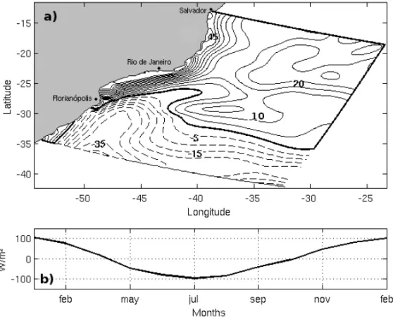
Figure 1 – (a) The study area and the annual mean surface heat flux; (b) time variation of the area-mean heat flux for the simulation domain.

possible choices presented above. The objective of the present work, carried out within the framework of the REMO network, is to investigate the impact that different formulations of the surface heat flux will have on the circulation in the ocean region adjacent to southeast Brazil. This study is carried out with realistic high-resolution simulations using the Regional Ocean Model System (ROMS). In the following section we present the model configu-ration and discuss the different heat flux formulations. Then re-sults are presented and discussed, focusing on the evolution of domain-averaged surface properties, and on the impact of fluxes upon the upwelling and upon individual eddies. Finally, the main conclusions are presented in the final section.

MODEL CONFIGURATION AND EXPERIMENTS

ROMS model (Shchepetkin & McWilliams, 2005) was configured from 14◦_{S to 34}◦_{S and 32}◦_{W to 52}◦_{W (Fig. 1), with ∼10km} horizontal resolution and 40 vertical sigma levels, with increased resolution near the surface. Bathymetry was derived from ETOPO2 (Global Gridded 2-minute Database), and initial conditions from WOA05 (World Ocean Atlas 2005) climatology (Locarnini et al., 2006; Antonov et al., 2006). Lateral boundaries are open via a radiational boundary condition and inflow conditions prescribed via temperature, salinity and geostrophic velocities derived from

WOA05. Surface wind stress and atmospheric variables used for computing surface fluxes are derived from COADS (Comprehen-sive Ocean-Atmosphere Data Set) monthly climatology (Slutz et al., 1985). Five experiments, differing in the way surface heat fluxes were formulated, were integrated for 5 years each. The spin up is very fast and the model is close to equilibrium conditions after the second year of simulation.

Experiment 1 is carried out without surface heat flux in order to provide a framework for comparison to the other experiments in which different flux formulations are tested. In experiment 2 climatological flux is prescribed, that is, there is no feedback of model SST upon the fluxes (corresponding to _T₁ = Tclim

and λ = 0). In experiment 3 heat flux is computed via relax-ation of model SST towards climatological SST (corresponding to

Q(T ) = 0 and T2= Tclim). In experiment 4, the flux is a

com-bination of prescribed climatological flux plus relaxation towards climatology (corresponding to_T₁_{= T}_climand_T₂_{= T}_clim). In experiment 5 fluxes (latent and sensible heat fluxes plus outgo-ing longwave radiation) are computed duroutgo-ing the simulation via bulk formulas using model SST and atmospheric variables (cor-responding to_T₁ = Tmodand λ = 0). Experiments and the

imposed heat flux setups are summarized in Table 1.

In all experiments, incoming solar radiation is allowed to pen-etrate into the ocean and to decay with depth following Paulson

(4)

“main” — 2014/1/3 — 18:13 — page 310 — #4

310

THE IMPACT OF SURFACE HEAT FLUXES ON THE SIMULATION OF THE BRAZIL CURRENT Table 1 – Model experiments.

Exp. 1 No flux Qnet= 0

Exp. 2 Climatological flux Qnet= Q(Tclim) Exp. 3 Relaxation to SST Qnet= λ(Tclim− T )

Exp. 4 Climatological flux Qnet= Q(Tclim)+ λ(T_clim− T ) plus relaxation to SST

Exp. 5 _{simulation via bulk formulas}Flux computed during the Qnet= Ql+ Qs+ Qb

& Simpson (1977). The relaxation parameter λ is calculated as the rate of change of net heat flux in relation to SST, and its value is associated to a decay scale of approximately 30 days. A virtual salinity flux replaces the physical mass flux given by evapora-tion and precipitaevapora-tion (E-P), and is formulated as a relaxaevapora-tion of model salinity (SSS) towards climatological sea surface salinity from WOA05. Although unrealistic from a physical point of view, since it implies a feedback of surface salinity upon surface fluxes, this approach has been justified (Bryan & Lewis, 1979; Holland & Bryan, 1994) since SSS is a generally more reliable field than E-P fluxes.

RESULTS

The simulated region is subjected to intense surface heat fluxes, with significant seasonal variability. Climatological surface heat loss (gain), reaching values higher than 100 W/m2, are observed within the entire domain during winter (summer) months, with a signature of the coastal upwelling (anomalous gain) presented in the fluxes for all months. On annual average, the region has a cold pattern in the southern part of the domain and warm pattern in northern part of the domain (Fig. 1), with a total warming trend of approximately 6 W/m2_{which should be compensated by lateral} oceanic fluxes for equilibrium to be reached.

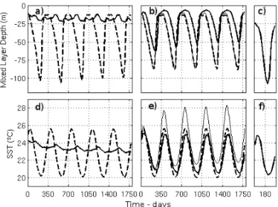
The ocean surface layers respond to the atmospheric forcing and a realistic seasonal cycle is simulated for SST field and mixed layer depth in all experiments, except for Exp. 1 (Fig. 2). Although the main circulation pattern is not strongly affected and a realistic BC flow is simulated in Exp. 1, as well as all the other experiments, without fluxes the SST and mixed layer depth tend to remain close to their initial conditions during the entire run (varying locally only due to horizontal advection). Exps. 5 and 4 have similar responses as expected, both for the SST and mixed layer, since the flux plus relaxation condition of Exp. 4 can be understood as a linear ap-proximation, in the sense discussed by Haney (1971), of the total fluxes computed in Exp. 5.

Experiment 2, with imposed climatological fluxes, presents warming and shallowing trends for the SST and mixed layer, re-spectively, as a response to the imbalance of the surface forcing over the model domain as discussed above (Fig. 2 (b) and (e)). Without any model feedback a realistic simulation of the surface thermal structure is difficult to achieve, and would be possible only for a perfect model with totally consistent boundary condi-tions. This problem should become more important and the de-parture from equilibrium conditions larger, for a longer simula-tion time.

Figure 2 – Time evolution of area-mean mixed layer depth (upper panels) and SST (lower panels). (a) and (d) for Exp. 1 (no flux – solid line) and Exp. 5 (bulk formula flux – dashed line); (b) and (e) for Exp. 2 (climatological flux – thin solid line), Exp. 3 (relaxation only – thick solid line) and Exp. 4 (climatological flux plus relaxation – dashed line); and (c) and (f) for observations derived from Argo floats climatology (http://mixedlayer.ucsd.edu/).

Experiment 3 on the other hand, with relaxation-only bound-ary conditions, is able to simulate realistic behavior and to impose a seasonal cycle upon the surface layers. The smaller amplitude of the mixed layer depth simulated in this case, when compared to the other runs (Fig. 2), is possibly related to the climatological SST field used for relaxation and should not be seem as a gen-eral rule for a relaxation condition. The most interesting aspect

(5)

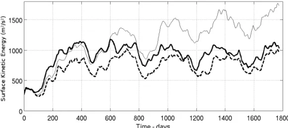
Figure 3 – Time evolution of domain-integrated surface kinetic energy per mass unit for Exp. 1 (thick solid line), Exp. 2 (thin solid line) and Exp. 5 (dashed line).

of this experiment, however, and one which is otherwise a direct consequence of the flux formulation, is the phase lag observed for both the SST and mixed layer as seen in Figure 2. Since the model is driven towards observed SST with a relaxation strength given by the value of λ (corresponding to a 30-day e-folding time in the present case), the simulated SST will always lag observa-tions (Pierce, 1996).

Stabilization of surface kinetic energy is achieved for all ex-periments, with the exception of Exp. 2, after the second year of integration (Fig. 3). The high values of kinetic energy simulated for this particular model domain reflect primarily the average flow of the BC-ICC system, as well as its intense mesoscale activity. It is a reassuring result, and one that is in line with the expected importance of mechanical forcing and of baroclinic instability for the region dynamics, that surface heat forcing formulation does not impact significantly upon the energy levels in Exps. 1, 3, 4 and 5.

In Exp. 2, however, with imposed fluxes, the kinetic energy continues to raise during the entire simulation, and an equilibrium is not obtained by the end of the 5-year model run. It is not clear

why imposed fluxes should lead to more intense energy levels. As seen in the surface TKE presented Figure 4, however, this behav-ior reflects the intensification in this particular experiment of the mesoscale activity associated with the BC-ICC system. It seems reasonable to suppose, therefore, that the thermal energy trend as-sociated with the surface forcing, as discussed above, somehow is transferred to available potential energy of the mean currents, affecting the instability process. Again, that does not seem to be a necessary consequence of imposed fluxes, and possibly reflects specific conditions of this particular model exercise. It is worth noting anyway, that heat flux formulation can have significant im-pact upon model dynamics and should be treated with care.

Another consequence of the way in which surface fluxes are implemented in the model for this particular domain is the be-havior of the coastal upwelling. The phenomenon, considered in its dynamical sense as the flow of subsurface waters invading the shelf towards the surface as a response to localized Ekman divergence associated with E-NE winds, is observed in all ex-periments. Additional experiments, not discussed here, show that the implementation of synoptic winds may represent an important

(6)

“main” — 2014/1/3 — 18:13 — page 312 — #6

312

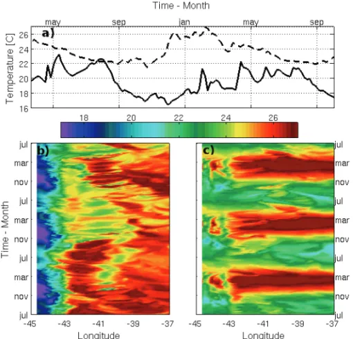
THE IMPACT OF SURFACE HEAT FLUXES ON THE SIMULATION OF THE BRAZIL CURRENT

Figure 5 – (a) SST time evolution at a point located at 23.3◦_{W and 44}◦_{W for Exp. 1 (solid line) and Exp. 5} (dashed line); (b) and (c) SST time evolution for a section at 23.3◦_{S for Exp. 1 and Exp. 5, respectively.}

factor for achieving the most intense cooling observed to occur in this region, but it is also clear from the present experiments that the process can be driven with reasonable realism with climato-logical winds.

Surface temperatures of upwelled waters, however, can be sig-nificantly influenced by the heat forcing. Actually, what is observed in the present model exercise is that only without surface heat fluxes (Exp. 1) the upwelling signal is significant at the surface (Fig. 5), with SST values below 17◦_{C. When fluxes are} imple-mented as in Exps. 2 to 5, SST cold anomalies associated with the upwelling are strongly damped and basically absent for all these runs, and SST never reaches below 21◦_{C near the coast.} The lack of a realistic SST feedback upon the atmospheric fields, and consequently upon the surface heat fluxes, does not allow SST anomalies to survive, although temperature anomalies below to approximately 20 meters are observed in all model runs. It is clear that the feedback considered in Exps. 3, 4 and 5 does not take into account the atmospheric response to the SST anomalies. The intense heating over the upwelling region, explicit in the climato-logical _Q_netand implicit in the atmospheric fields used in the bulk formulation of Exp. 5, does not allow for the maintenance of the cold SST anomalies in these model runs. The situation is

para-doxical, since only the case with unrealistic SST over the model domain can achieve realistic SST in the upwelling region.

The situation becomes even more complex when the behav-ior of the upper ocean thermal structure within eddies generated by the BC-ICC system is taken into consideration. In regions of intense currents the upper ocean heat balance has to take into account both the surface fluxes and the horizontal advection. Ad-vection will be of particular importance during the eddy generation and shedding process, which in this region will be prominent off Cabo Frio and S˜ao Tom´e, where eddy formation is recurrent. What we found in our experiments can be summarized as:

a) with or without surface heat fluxes, and independently of formulation, eddy generation process is vigorous and take place in the expected regions (as discussed above, Exp. 2 presents an intensification of mesoscale activity, while surface TKE is very similar for all the other cases); b) by considering the surface heat flux into the model it has

an important impact upon the upper ocean thermal struc-ture even within eddies, where advection is a dominant process, and change significantly the vertical shear of up-per layers.

(7)

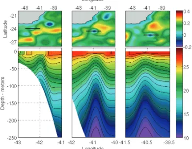
This behavior is exemplified in Figures 6 and 7, in which two similar Cabo Frio eddies are compared for Exp. 1, without fluxes, and Exp. 5, with fluxes computed via bulk formulas. Exps. 2, 3 and 4 present behaviors similar to Exp. 5, and the particular ed-dies discussed are representative of all eded-dies generated without (Fig. 6) and with (Fig. 7) surface heat fluxes. Both eddies are gen-erated at the border of the continental shelf, and move towards deeper waters. Without fluxes, horizontal temperature and density gradients, and therefore vertical shear is intense even very close to the surface. With fluxes the eddy formation is very similar at the first days, but after 15 days and most prominent after 30 days hor-izontal temperatures gradients are significantly reduced and even-tually completely lost in the first 20 meters of the water column, changing the current shear. Even if the impact of heat fluxes seem to be restrict to the very upper layers, it is just the currents near the surface that are of particular importance for environmental prob-lems and are, therefore, the ones that REMO is mostly concerned with. The results with imposed fluxes are more realistic, and it is not uncommon in remote sensing analysis to observe eddies that maintain a strong signal in sea surface height from altimetry, but that lose its sea SST signature a few days after being generated.

Figure 6 – Surface elevation (upper panels) and Lagrangian temperature sec-tions at the center of a Cabo Frio eddy for the same instant (lower panels) for Exp. 1. Difference of 15 days between each section.

CONCLUSIONS

In the present paper a numerical study was carried out dealing with the impact of surface heat flux formulation on the simulation of the Brazil Current. In summary, we can say that:

a) with or without fluxes an intense and baroclinic unsta-ble BC can be simulated, with realistic mean flow and mesoscale variability;

b) taken the surface heat fluxes into account is essential for a correct simulation of the thermal structure of the upper ocean, even in regions of intense horizontal advection and within BC eddies;

c) SST signal at the Cabo Frio upwelling may be strongly damped by the heat fluxes, what is possibly related to ab-sence of realistic feedback of simulated SST upon atmo-spheric variables and upon the surface fluxes;

d) imposing climatological fluxes may lead to unrealistic simulations, in particular for long runs in which there is no control upon SST drifts, and some feedback is neces-sary even if the atmosphere is not allowed to respond to SST;

e) fluxes computed via pure relaxation of SST towards ob-served (climatological) values lead to a seasonal cycle of SST and mixed layer depth that lags observations, the value of the lag being related to the value of the relaxation constant;

f) Computing fluxes with bulk formulas is similar to impos-ing climatological fluxes plus a relaxation of SST towards climatology, since this last approach can be understood as a linear approximation of the total fluxes.

It is important to notice that some of the behavior described here may by quantitatively or even qualitatively different if different cli-matological data sets are used, or if the synoptic scale is taken into account, for instance.

Figure 7 – Surface elevation (upper panels) and Lagrangian temperature sec-tions at the center of a Cabo Frio eddy for the same instant (lower panels) for Exp. 5. Difference of 15 days between each section.

(8)

“main” — 2014/1/3 — 18:13 — page 314 — #8

314

THE IMPACT OF SURFACE HEAT FLUXES ON THE SIMULATION OF THE BRAZIL CURRENT Not much can be found in the literature regarding the impor-tance of heat flux to the modeling of the Brazil Current, but the issue of heat flux formulation has draw some attention regarding ocean circulation in general. Traditionally, ocean modelers have opted for restoring boundary conditions (e.g., Han, 1984; Bryan, 1986; Holland & Bryan, 1994; Barnier et al., 1999), while more recent studies have favored the use of atmospheric data in the heat flux formulation, applying either a Haney-type formulation (e.g., Gulev et al., 2003) or directly the bulk formulas (e.g., Srini-vasan et al., 2011). This results from an improved confidence in the atmospheric data and from a general belief (Large et al., 1997), not necessarily totally justifiable (Seager et al., 1995), that more physically consistent boundary conditions will lead to more realistic model results. Our experience in REMO, based also in previous studies (Paiva & Chassignet, 2001) has shown that the use of a combination of bulk formulation plus a restoring term (Gabioux et al. 2013, this issue) leads in general to better results in the modeling of the South Atlantic ocean basin.

As mentioned before, none of the formulations for surface heat flux usually employed in numerical ocean models, and tested here, accounts perfectly for the physical processes involved in the air-sea interaction. Surface heat fluxes, however, represent an im-portant component of the atmospheric forcing and have to be taken into consideration in one or another form. Our results point to the importance of a careful consideration of the thermal surface forc-ing, and of its formulation, for a realistic simulation of the flow in the oceanic region adjacent to southeast Brazil. It is possible that a more realistic feedback may be necessary even for regional simulations like the ones performed here.

ACKNOWLEDGMENTS

The authors wish to thank to GruPO (Grupo de estudos de Pro-cessos Oceânicos, from COPPE/UFRJ) for a continuous and stimulating discussion. This research was supported by REMO (Rede de Modelagem e Observação Oceanográfica).

REFERENCES

ANTONOV JI, LOCARNINI RA, BOYER TP, MISHONOV AV & GARCIA HE. 2006. World Ocean Atlas 2005, Volume 2: Salinity. S. Levitus, Ed. NOAA Atlas NESDIS 62, U.S. Government Printing Office, Washington, D.C., 182 pp.

BARNIER B, MARCHESIELLO P, MIRANDA APD, MOLINES JM & COULIBALY MA. 1999. Sigma-coordinate primitive equation model for studying the circulation in the South Atlantic. Part I: Model configuration with error estimates. Deep-Sea Research, 45: 543–572.

BRYAN FO. 1986. High latitude salinity effects and interhemispheric thermohaline circulations. Nature, 323: 301–304.

BRYAN K & LEWIS LJ. 1979. A water mass model of the world ocean. Journal of Geophysical Research, 84: 2503–2517.

CALADO L, GANGOPADHYAY A & SILVEIRA ICA. 2006. A Parametric Model for the Brazil Current Meanders and Eddies off Southeastern Brazil. Geophysical Research Letters, 33: L12602.

CALADO L, SILVEIRA ICA, GANGOPADHYAY A & DE CASTRO BM. 2010. Eddy-induced upwelling off Cape S˜ao Tom´e (22◦_{S, Brazil). Continental} Shelf Research, 30: 1181–1188.

CASTEL˜AO RM & BARTH JA. 2006. Upwelling around Cabo Frio, Brazil: The importance of wind stress curl. Geophysical Research Let-ters, 33: L03602.

CHU PC, CHEN Y & LU S. 1998. On Haney-type surface thermal boundary conditions for ocean circulation models. Journal of Physical Oceanography, 28: 890–901.

FERNANDES AM, SILVEIRA ICA, CALADO L, CAMPOS EJD & PAIVA AM. 2009. A two-layer approximation to the Brazil Current – Intermedi-ate Western Boundary Current System between 20◦_{S and- 28}◦_{S. Ocean} Modeling, 29: 154–158.

GABIOUX M, COSTA VS, SOUZA JMAC, OLIVEIRA BF & PAIVA AM. 2013. Modeling the South Atlantic Ocean from medium to high reso-lution. Revista Brasileira de Geof´ısica, 31(2): 229–242.

GULEV SK, BARNIER B & KNOCHEL H. 2003. Water Mass Transforma-tion in the North Atlantic and Its Impact on the Meridional CirculaTransforma-tion: Insights from an Ocean Model Forced by NCEP-NCAR Reanalysis Sur-face Fluxes. Journal of Climate, 16(19): 3085–3110.

HAN YJ. 1984. A numerical world ocean general circulation model. Part I: Basic design and barotropic experiment. Dynamics of Atmospheres and Oceans, 8: 107–140.

HANEY RL. 1971. Surface Thermal Boundary Condition for Ocean Cir-culation Models. Journal of Physical Oceanography, 1(4): 241–248. HOLLAND WR & BRYAN FO. 1994. Modeling the wind and thermoha-line circulation in the North Atlantic Ocean. Ocean Processes in Climate Dynamics: Global and Mediterranean Examples, P. Malanotte-Rizzoli and A. Robinson, Eds., Kluwer Academic: 135–156.

KILLWORTH PD, SMEED DA & NURSER AJG. 2000. The effects on ocean models of relaxation toward observation at the surface. Journal of Phys-ical Oceanography, 30: 160–174.

LARGE W, DANABASOGLU G, DONEY SC & McWILLIAMS JC. 1997. Sensitivity to surface forcing and boundary layer mixing in a global ocean model: Annual mean climatology. Journal of Physical Oceanography, 27: 2418–2447.

LOCARNINI RA, MISHONOV AV, ANTONOV JI, BOYER TP & GARCIA HE. 2006. World Ocean Atlas 2005, Volume 1: Temperature. S. Levitus, Ed.

(9)

NOAA Atlas NESDIS 61, U.S. Government Printing Office, Washington, D.C., 182 pp.

MANO M, PAIVA AM, TORRES Jr AR & COUTINHO ALGA. 2009. En-ergy flux to a Cyclonic Eddy off Cabo Frio, Brazil. Journal of Physical Oceanography, 39(11): 2999–3010.

MIRANDA LB. 1985. Forma da Correlação T-S de Massas de Água das Regiões Costeira e Oceânica entre o Cabo de São Tomé (RJ) e a Ilha de São Sebastião (SP). Bolm Inst. Oceanogr., S. Paulo, 33(2): 105–119. MOREIRA DA SILVA PC & MENDONÇA CF. 1977. Origem da Água da ressurgência em Cabo Frio. Instituto de Pesquisa da Marinha, 114 pp. MÜLLER TJ, IKEDA Y & ZANGENBERG N. 1998. Direct Measurements of Western Boundary Currents off Brazil between 20◦_{S and 28}◦_{. Journal} of Geophysical Research, 103: 5429–5437.

PAIVA AM & CHASSIGNET EP. 2001. The Impact of Surface Flux Pa-rameterizations on the Modeling of the North Atlantic Ocean. Journal of Physical Oceanography, 31: 1860–1878.

PAULSON CA & SIMPSON JJ. 1977. Irradiance measurements in the upper ocean. Journal of Physical Oceanography, 7: 952–956. PIERCE DW. 1996. Reducing phase and amplitude errors in restoring boundary conditions. Journal of Physical Oceanography, 26: 1552– 1560.

RODRIGUES RR & LORENZZETTI JA. 2001. A numerical study of the effects of bottom topography and coastline geometry on the Southeast Brazilian coastal upwelling. Continental Shelf Research, 21: 371–394.

SEAGER R, KUSHNIR Y & CANE MA. 1995. On heat flux boundary con-ditions for ocean models. Journal of Physical Oceanography, 25: 3219– 3230.

SHCHEPETKIN AF & McWILLIAMS JC. 2005. The regional oceanic modeling system (ROMS): a split-explicit, free-surface, topography-following-coordinate oceanic model. Ocean Modelling, 9: 347–404. SILVEIRA ICA, SCHMIDT ACK, CAMPOS EJD, GODOI SS & IKEDA Y. 2000. The Brazil Current off the Eastern Brazilian Coast. Revista Brasi-leira de Oceanografia, 48(2): 171–183.

SILVEIRA ICA, CALADO L & CASTRO BM. 2004. On the Baroclinic Structure of the Brazil Current-Intermediate Western Boundary Current at 22◦_-23◦_{S. Geophysical Research Letters, 31, L14308.}

SILVEIRA ICA, LIMA JAM, SCHMIDT ACK, CECCOPIERI W, SARTORI A, FRANCISCO CPF & FONTES RFC. 2008. Is the meander growth in the Brazil current system off Southeast Brazil due to baroclinic instability? Dynamics of Atmospheres and Oceans, 45: 187–207.

SLUTZ RJ, LUBKER SJ & HISCOX JD. 1985. Comprehensive Ocean-Atmosphere Data Set; Release 1. NOAA Environmental Research Lab-oratories, Climate Research Program, Boulder, CO, 268 pp.

SRINIVASAN A, CHASSIGNET EP & BERTINO L. 2011. A comparison of sequential assimilation schemes for ocean prediction with the HYbrid Coordinate Ocean Model (HYCOM): Twin experiments with static fore-cast error covariances. Ocean Modelling, 37: 85–111.

STRAMMA L & ENGLAND M. 1999. On the Water Masses and Mean Circulation of the South Atlantic Ocean. Journal of Geophysical Re-search, 104(C9): 20863–20883.

Recebido em 10 abril, 2012 / Aceito em 21 novembro, 2012 Received on April 10, 2012 / Accepted on November 21, 2012

NOTES ABOUT THE AUTHORS

Vladimir Santos da Costa. Graduated in Physics from the Universidade Federal Rural do Rio de Janeiro (2005), and M.Sc. in Ocean Engineering from the Universidade Federal do Rio de Janeiro – UFRJ (2008). Currently is a doctoral student at Program of Ocean Engineering of COPPE/UFRJ, developing studies on air-sea interaction, mesoscale variability in the ocean, and data assimilation in ocean models.

Afonso de Moraes Paiva. Graduated in Oceanography from the Universidade Estadual do Rio de Janeiro (1985), M.Sc. in Ocean Engineering from the Univer-sidade Federal do Rio de Janeiro (1992), and Ph.D. Physical Oceanography from the Rosenstiel School of Marine and Atmospheric Sciences of University of Miami (1999). Currently is a professor at the Program of Ocean Engineering of COPPE/UFRJ. Main research interestes are: geophysical fluid dynamics, thermodynamic processes in the oceans and ocean-atmosphere interaction, meso and large scale ocean circulation, climate variability, and numerical modeling of ocean circulation.