Universidade de Lisboa
Faculdade de Ciências
Departamento de Engenharia Geográfica, Geofísica e Energia
Continental Surface Water and Energy Budgets in
the XX and XXI Centuries
Sandra Maria de Carvalho Gomes
Doutoramento em Ciências Geofísicas e da
Geoinformação
(Meteorologia)
2014
Universidade de Lisboa
Faculdade de Ciências
Departamento de Engenharia Geográfica, Geofísica e Energia
Continental Surface Water and Energy Budgets in
the XX and XXI Centuries
Contents
Contents
Contents ... i Acknowledgements ...v Resumo ... vi Abstract ... viiiList of acronyms and abbreviations ... ix
Chapter 1 - Introduction ...1
1.1 Motivation and brief state of the art...1
1.2 Overview of water and energy budget ...4
1.2.1 Global hydrological cycle ...4
1.2.2 Surface energy budgets ...5
1.3 Research objectives and thesis organization ...7
Chapter 2 - The land surface model and forcing data in the presence of reanalysis...9
2.1 Introduction ...9
2.2 Correction for rainfall and snowfall rate ... 10
2.2.1 Wet days correction ... 11
2.2.2 Monthly bias correction ... 12
2.2.3 Maximum precipitation: outliers ... 13
2.2.4 Correction for gauge undercatch... 14
2.3 Land Surface Model – HTESSEL and CTESSEL ... 16
2.3.1 TESSEL hydrology ... 16
2.3.2 Soil water budget ... 17
2.3.3 H-TESSEL and snow revisions ... 18
2.3.4 The C-TESSEL ... 18
2.3.5 Model Versions ... 18
2.4 Evaluation of the land surface model HTESSEL against FLUXnet data ... 19
2.4.1 FLUXNET sites ... 19
2.4.2 Site and observations ... 20
2.5 Conclusions ... 23
Contents
ii
3.5.2 Precipitation disaggregation ... 32
3.5.3 Total disaggregation ... 33
3.6 Balance of water and energy over land ... 34
3.6.1 Global water and energy cycle impact ... 35
3.7 Conclusions ... 38
Chapter 4 - Current state of climate... 39
4.1 Modelling of land surface processes ... 39
4.1.1 Offline global simulations ... 41
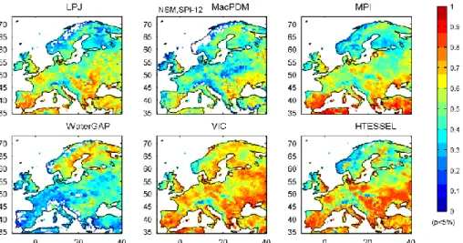
4.1.2 Multimodel analysis: hydrological cycle ... 42
4.1.3 Multimodels results ... 57
4.2 Sensitivity study ... 58
4.2.1 Methodology and data ... 58
4.2.2 Analysis of the global energy balance ... 59
4.2.3 Comparison of observed and simulated data: a site analysis... 64
4.2.4 Concluding remarks – energy cycle ... 67
Chapter 5 - Global change in future climate ... 69
5.1 Global warming and hydrology ... 69
5.1.1 Climate impacts – Water in the future ... 70
5.2 Simulated historical and projected climate ... 70
5.3 Temporal fields ... 71
5.4 Annual and seasonal regimes ... 72
5.4.1 Air temperature and precipitation ... 72
5.4.2 Total runoff variability ... 76
5.4.3 Soil moisture ... 77
5.4.4 Energy budget ... 78
5.4.5 Climate variables controlling surface hydrology ... 79
5.5 Changes in spatial distribution in European climate ... 80
5.5.1 Soil moisture-precipitation feedback ... 83
5.5.2 Present and future evapotranspiration and total runoff over Europe ... 84
5.6 Global patterns of changing extremes ... 86
5.6.1 Precipitation extremes ... 86
5.6.2 Precipitation return periods ... 87
5.7 Conclusions ... 88
Chapter 6 - Final Discussion and Conclusions ... 89
6.1 General Conclusions... 89
6.2 Recommendations for Future Work ... 91
Contents
Appendix I - Statistical indicators of accuracy ... 103
Appendix II - GLM Stochastic Weather Generator ... 105
II.1 Weather Generators ... 105
II.1.1 Application to daily weather ... 106
II.1.2 Summary description ... 109
II.2 Model Fitting ... 109
II.2.1 Global modelling calibration ... 110
II.2.2 Performance of GLM modelling ... 112
II.2.3 HTESSEL modelling ... 115
II.3 General discussion and conclusions ... 119
Appendix III - GEV Distribution ... 121
III.1 L Moments ... 122
III.2 Maximum Likelihood Estimators ... 122
Acknowledgements
Acknowledgements
At the end of my thesis, it is a pleasant task to express my thanks to all those who contributed in many ways to the success of this study and made it an unforgettable experience for me. This thesis has been kept on track and been seen through to completion with the support and encouragement of numerous people including my friends, family, colleagues and various institutions.
My first acknowledgement goes to Doctor Pedro Viterbo, my PhD supervisor. His guidance and support during the long period of this work were important to overcome the several difficulties that arose. His belief in the successful completion of this thesis and the logistic support were essential. Thanks to my co-supervisor Professor Doctor Pedro Miranda and Dr Graham Weedon from the Centre for Ecology & Hydrology (CEH).
To “Fundação para a Ciência e a Tecnologia” (FCT) I am grateful for the financial support through a PhD scholarship (SFRH/BD/76852/2011). I am also indebted to the financial support from Integrated Project Water and Global Change (WATCH, 2007-2011), funded under the EU FP6 and to the logistic support of “Faculdade de Ciências da Universidade de Lisboa” (FCUL), “Instituto Dom Luiz” (IDL) and “Instituto Português do Mar e da Atmosfera” (IPMA). I would like to express a special thanks to all colleagues from IPMA and IDL.
Dear Mum, Dad and my siblings it is hard to express my thanks to you in words. Your understanding, the faith, advise, intellectual spirit and indescribable support to me throughout my whole life are invaluable. Last but not least, I would like to pay high regards to my husband José, who listened and discussed ideas about this thesis with me on many occasions, and my son Jorge for their sincere encouragement and inspiration throughout my research work and lifting me uphill this phase of life. I owe everything to them. To my son by his lovely smile. Their guidance and support during the long period of this work were important to overcome the several difficulties that arose. Their belief in the successful completion of this thesis and the logistic support were essential.
Besides this, several people have knowingly and unknowingly helped me in the successful completion of this project.
Resumo
vi
Resumo
Diversos estudos emergiram nas últimas décadas tendo em vista a caracterização e estimativa do ciclo hidrológico terrestre bem como do ciclo energético. O Programa GEWEX (“Global Energy and Water Cycle Experiment”), iniciado nos anos 90 do século XX, tem sido a entidade que enquadra estas atividades a nível global e continental; o projeto FP5 WATCH (“WATer and global CHange”), no qual esta tese está inserida, contribuiu para o conhecimento, caracterização e previsão de variações no ciclo hidrológico e energético à superfície nos séculos XX e XXI, bem como alterações nos processos hidrológicos e dos recursos hídricos a escalas regionais.
Uma das formas de caracterizar as trocas de água à superfície é o recurso a observações in-situ capazes de reproduzir séries hidrológicas. As observações in-situ, limitadas a pontos de medidas de caudais de cursos de água, podem ser complementadas por modelos de superfície forçados por séries meteorológicas. Os primeiros registos de observações de variáveis meteorológicas começaram a surgir, à escala continental, há cerca de 120 anos. Atualmente existem sínteses de observações mensais, para todo o globo desde o início do século XX, por exemplo o conjunto de dados da CRU (“Climatic Research Unit”) e do GPCC (“Global Precipitation Climatology Centre”), disponibilizando séries mensais de precipitação, entre outras variáveis, no caso do CRU. Para compensar a irregularidade na distribuição espacial de observações surgiram as reanálises obtidas por assimilação multivariada de dados provenientes de diversas fontes (medições in-situ, radiosondas e deteção remota) combinadas com estimativas a priori de modelos de previsão. Exemplos incluem as reanálises da NASA (“National Aeronautics and Space Administration”), do NCEP (“National Centers for Environmental Prediction”), do ECMWF (“European Centre for Medium-Range Weather Forecasts”) e do JMA (“Japan Meteorological Agency”). Muitos dos dados utilizados atualmente para forçar modelos de superfície foram construídos a partir de reanálises disponíveis essencialmente para a segunda metade do século XX até à atualidade. Os erros sistemáticos inerentes às reanálises são minimizados quando corrigidos com as observações disponíveis. Bases de dados globais a 1 grau de resolução incluem: NCC, construída para 1948-2000 a partir da reanálise do NCEP/NCAR; e PGF (“Princeton Global Forcing”), corrigida pelas observações do CRU. O projeto WATCH produziu a WFD (“WATCH Forcing Data”) recriada a partir da reanálise ERA-40 e das observações do CRU e GPCC. A WFD tem uma resolução espacial de 0.5 graus, gerada em 67420 pontos de terra (excluindo a Antártica) e disponibiliza cinco variáveis com 6h de resolução temporal e os fluxos a 3h. A primeira metade do século XX, onde é bastante mais difícil recriar reanálises de boa qualidade devido à insuficiência dos sistemas de observação, pode ser reproduzida através de métodos estatísticos e de desagregação diária aplicados a estimativas mensais. Os “weather generators” estocásticos produzem séries temporais de dados meteorológicos sintéticos para um determinado local de acordo com as características estatísticas das variáveis. Paralelamente surgiram os modelos lineares generalizados (GLM – “Generalized Linear Model”), que permitem a estimativa de uma variável através de uma combinação linear de covariáveis. A aproximação GLM pode ser aplicada a um “weather generator” paramétrico, para várias variáveis no mesmo local simultaneamente. De modo a poder aplicar os resultados obtidos pelo GLM foi necessário desenvolver métodos de desagregação diária que permitem a utilização desses dados para forçar modelos de superfície.
O clima futuro, essencial para a representação do ciclo da água no século XXI, pode ser estimado recorrendo a modelos de circulação atmosférica. O projeto WATCH disponibiliza forçamento atmosférico diário à escala global, 0.5º apenas pontos de terra, para o clima atual [1960-2000] e cenários B1 e A2 [2001-2100] do quarto relatório do IPCC, fornecendo as condições necessárias para guiar modelos hidrológicos e modelos de superfície. Nesta tese, o forçamento resulta da projeção de três modelos atmosfera-oceano acoplados (ECHAM5/MPIOM, CNRM-CM3 e LMDZ-4) seguindo os cenários de emissão B1 (otimista) e A2 (pessimista) do IPCC. Devido aos erros sistemáticos inerentes aos resultados dos modelos climáticos, foi aplicada uma correção estatística ao output de forma a eliminar o viés, podendo assim ser posteriormente utilizado como forçamento de modelos hidrológicos
Resumo globais e calcular as variações no ciclo hidrológico e fluxos de energia em vários cenários do clima futuro.
Dependendo do objetivo, os modelos hidrológicos são divididos em duas categorias: modelos de superfície (LSM – “Land Surface Models”) e modelos de balanço de água (WBM – “Water Balance Models”), também denominados modelos hidrológicos globais (GHM – “Global terrestrial Hydrological Models”). Nos modelos GHMs o ciclo da água é tratado de forma conceptual, enquanto os LSMs resolvem tanto o balanço água como o de energia. Para além disso os dois tipos de modelos podem diferir na resolução espacial e temporal, detalhes nos processos, número de parâmetros e de dados necessários. Apesar destas diferenças tanto os GHMs como os LSMs são usados para estimar variáveis de estado hidrológicas e fluxos de água e energia. De modo a analisar as incertezas associadas ao ciclo da água, diferentes comunidades (hidrologia, meteorológica e de clima) juntaram-se de modo a comparar resultados e criar um ensemble de dados a partir de diferentes modelos. A intercomparação de modelos (PILPS, ALMIP, GSWP2, WaterMIP) permite a avaliação da incerteza associada a diversos fatores, entre eles as parametrizações próprias de cada modelo.
Esta tese está dividida em duas partes: desenvolvimento de dados de forçamento para modelos hidrológicos; respetiva validação e estimativa do ciclo hidrológico e energético nos séculos XX e XXI. O forçamento é utilizado pelos modelos de superfície, o que permitiu a criação de um ensemble de modelos hidrológicos (GHMs e LSMs)) contribuindo para a caracterização da hidrologia em ambos os séculos e da estimativa da incerteza associada. A base de dados de forçamento meteorológico, desenvolvida no âmbito do projeto WATCH, é uma base de dados longa e globalmente consistente de variáveis meteorológicas utilizada para conduzir modelos hidrológicos. A coerência da base de dados foi testada em simulações hidrológicas com alguns dos modelos hidrológicos participantes no projeto de intercomparação de modelos do WATCH (WaterMIP), para o qual esta tese contribuiu com simulações HTESSEL, um LSM. De modo a caracterizar o balanço de energia, foram feitos vários testes de sensibilidade ao forçamento e às parametrizações físicas do modelo.
Paralelamente foi utilizado o forçamento atmosférico proveniente de modelos climáticos para os séculos XX e XXI (clima atual e cenários B1 e A2) estimado por modelos climáticos que fornecem as condições necessárias para guiar modelos hidrológicos em cenários futuros. A componente terrestre do ciclo hidrológico foi avaliada e analisada focando no período [2071-2100] e comparada com o clima presente [1971-2000]. Nesta tese foram apenas apresentados os resultados das simulações com o modelo de superfície HTESSEL conduzido com o forçamento proveniente do modelo de circulação global ECHAM para o clima presente e os cenários futuros B1 e A2. Aspetos hidrológicos associados a eventos extremos de seca e precipitação intensa nos séculos XX e XXI, foram igualmente analisados.
Os resultados obtidos permitem a caracterização dos ciclos hidrológico e energético à superfície em ambos os séculos. O ciclo hidrológico, apresentado apenas para o período 1985 a 1999, foi comparado com cinco modelos hidrológicos integrantes no projeto WaterMIP. A precipitação sobre os continentes estimada é de 880 mm/ano, dos quais 510 mm são libertados para a atmosfera devido ao processo de evapotranspiração e 368 mm de escoamento superficial e subterrâneo. O balanço de energia à superfície foi igualmente calculado e avaliado. A radiação disponível à superfície tem um saldo de aproximadamente 70 Wm-2, dos quais 24 Wm-2 são libertados para a atmosfera sobre a forma de fluxo
Abstract
viii
Abstract
The global water cycle is an integral part of the Earth system, playing a central role in our climate and controlling the global energy cycle as well as carbon, nutrient, and sediment cycles.
The development of hydrological models and respective driving forcing allows a better knowledge of the land surface. There are a diversity of hydrological models and approaches, ranging from conceptually based lumped models to distributed physically based hydrology models. This range was developed in response to many different requirements in terms of scale, purpose, and availability data. Model intercomparison efforts have helped to reveal the strengths and weaknesses of the individual models. This exercise provides useful feedback to modellers and improved our understanding of the water cycle. Aspects like seasonal and interannual behaviour were analysed improving our knowledge about the land surface modelling. The methods and datasets developed in this thesis allow us to make estimates of past and future global water availability. The forcing data were used as input to hydrological and land surface models to produce comprehensive global water cycle data sets, which were also validated. The global water cycle data sets also provided invaluable historical data for areas of the world where little data or no observed climate and hydrological data exist.
The first step was the production of the WATCH Forcing Data, merging a 3-hourly reanalysis and monthly observations. The forcing data were then used as input to hydrological and land surface models, producing an ensemble of global water and energy cycle datasets. The use of this data assessed the hydrology of continental surface, focus on Europe.
The main purpose of this thesis was to provide a more consistent analysis of components of the terrestrial surface water and energy budgets for the twentieth and twentieth-first centuries. The forcing data is available to everyone.
Keywords: Surface hydrological and energy cycles, land surface, land surface models, atmospheric forcing, climate change
List of acronyms and abbreviations
List of acronyms and abbreviations
20C3M 20th Century Climate in Coupled Models
AGCM Atmosphere General Circulation Model
AIC Akaike information criterion
ALMIP AMMA – Land surface Model Intercomparison Project AMMA African Monsoon Multidisciplinary Analysis
AR4 IPCC Fourth Assessment Report
AR5 IPCC Fifth Assessment Report
BIC Bayesian Information Criterion
CNRM-CM3 Centre National de Recherches Météorologiques Coupled Model Version 3
CR Catch Ratio
CRU Climate Research Unit
CTESSEL Carbon Tiled ECMWF Scheme for Surface Exchanges over Land
DDM Daily Disaggregator Method
DJF December, January and February
ECHAM5/MPIOM ECMWF and Hamburg (Coupled climate model consisting of atmospheric general circulation model and MPI-OM ocean-sea ice component developed at the Max Planck Institute for Meteorology - MPIM).
ECMWF European Centre for Medium-Range Weather Forecasts
EI El Niño index
ENSO El Nino-Southern Oscillation
ERA-40 ECMWF 40-years reanalysis
ERAI ECMWF Interim reanalysis
ESPI ENSO precipitation index
FLUXNET Global Network of Flux Towers
GCIP GEWEX Continental Scale International Project
GCM General Circulation Model
GEWEX Global Energy and Water Cycle Experiment GHM Global terrestrial Hydrological Models
GLM Generalized Linear Models
GPCC Global Precipitation Climatology Centre GPCP Global Precipitation Climatology Project
GSWP Global Soil Wetness Project
GWSP Global Water System Project
HTESSEL Hydrology Tiled ECMWF Scheme for Surface Exchanges over Land
IFS Integrated Forecast System
IPCC Intergovernmental Panel on Climate Change
ISLSCP International Satellite Land Surface Climatology Project ITCZ Inter-tropical Convergence Zone
List of acronyms and abbreviations
x NCAR National Center for Atmospheric Research
NCEP National Centers for Environmental Prediction
NSM Normalized Soil Moisture
NWP Numerical weather prediction
OGCM Oceanic General Circulation Models
PDSI Palmer Drought Severity Index
PGF Princeton Global Forcing
PILPS Project for the Intercomparison of Land-Surface Parameterization Schemes
SON September, October and November
SPI Standard Precipitation Index
SRES Special Report on Emission Scenarios
TESSEL Tiled ECMWF Scheme for Surface Exchanges over Land
TWS Terrestrial Water Storage
VIC Variable Infiltration Capacity model
WATCH WATer and global CHange
WaterGAP Water - Global Assessment and Prognosis WaterMIP Water Model Intercomparison Project
WFD WATCH Forcing Data
Chapter 1 - Introduction
Chapter 1 - Introduction
1.1 Motivation and brief state of the art
Peixoto and Oort (1992) defined the global hydrosphere as various reservoirs connected by the transfers of water in the various phases, playing a central role in the Earth climate system. The hydrological cycle has two major branches. The terrestrial branch consists of the inflow, outflow, and storage of water in its various forms on and in the continents and oceans, while the atmospheric branch consists of the atmospheric transports of water, mainly in the vapour phase. The two branches of the hydrological cycle communicate at the atmosphere-earth surface interface.
The Earth climate fluctuates and changes both regionally and globally. These changes are reflected in the variability and change of Earth’s water budget and the complex and dynamic energy balance. The first description of the energy budget for the Earth was proposed by Dines (1917). Over the last two decades, improvements in estimating the global annual mean energy budget have resulted from satellite observations (Kiehl and Trenberth, 1997; Fasullo and Trenberth, 2008a, 2008b; Trenberth and Fasullo, 2008; Trenberth et al., 2009; Trenberth et al., 2011). Recently, an assessment of the global energy and hydrological cycles from eight current atmospheric reanalyses and their depiction of changes over time were made by Trenberth et al. (2011). Early studies of the water cycle include Chahine (1992), and Oki (1999); Peixoto and Oort (1992) provided an estimated global water cycle partly based on their computations for atmospheric vapour transport. Oki (1999) compiled a water cycle based on estimates of atmospheric transports from ECMWF and precipitation data. However, there are still very few studies on a global scale, providing a synthesis of the mean and variability of the global water cycle, and corresponding error estimates (Oki and Kanae 2006; Trenberth et al. 2007; Trenberth et al. 2011; Trenberth and Asrar 2014). Due to the scarcity of data on a global scale of its various components, e.g., precipitation, surface evapotranspiration, terrestrial runoff, our knowledge of the global cycle is limited. Sheffield et al. (2010) study was a first step in quantifying the long-term variation in global land evapotranspiration from remote sensing data. Nevertheless satellite data do not adequately close the water budget at regional scale (Gao et al., 2010; Sheffield et al., 2010; Vinukollu et al., 2011; Sahoo et al., 2011).
The terrestrial hydrological cycle is an important component of the global climate and biospheric system, influencing the climate in a variety of ways. The water is recycled in a continuous process known as the water cycle. Exchanges of moisture and energy between the atmosphere and the Earth’s surface affect the dynamics and thermodynamics of the climate system. In the forms of vapour, cloud liquid and ice water, rain, snow and hail, as well as during phase transitions, water plays opposing roles in heating and cooling the environment. The energy from the Sun triggers the global movement of water, the water cycle. The Sun’s differential heating, varying with latitude and time of the year, drives a continuous exchange of water among the reservoirs. On the other hand, the exchange pathways are controlled by surface properties and atmospheric and ocean circulation.
Water and energy cycles are expressed with similar equations (Seneviratne et al., 2010). They are both governed by conservation laws for water mass and energy. Cycles have similar components: storage and transport terms. The storage terms represent the great reservoirs of water and energy, and the transport
Chapter 1 - Introduction
2 The water cycle is a closed system: the volume of water in the hydrosphere today is the same amount of water that has always been present in the Earth system. Water evaporated from the oceans, lakes, river, or soil is driven by solar energy. In addition, water moves from plants to the atmosphere due to transpiration. It forms water vapour and clouds, which eventually comes back to Earth as rain, snow, dew or hail, or other forms of precipitation. Precipitation runs at surface as runoff or as ground water, and eventually, back into the surface reservoirs. Rain or melt water may be intercepted by vegetation cover or retained by land surface depressions, may infiltrate into the soil, or may run over the land surface into streams. Infiltrated water may be stored in the soil as soil moisture or may percolate to deeper layers to be stored as groundwater. During cold periods a portion of infiltrated water may freeze in the soil. Part of water intercepted by vegetation, accumulated in land surface depressions, and stored in the soil, may return back to the atmosphere as a result of evaporation. Plants take up a significant portion of the soil moisture from the root zone and evaporate most of this water through their leaves. In addition to the redistribution of water, the hydrological cycle is also responsible for the absorption and redistribution of solar energy from one location to another. Latent heat release occurs when condensed (liquid or soil) water transforms to vapour and plays a fundamental role in the Earth’s radiation balance. Evaporation absorbs energy from the surface and releases it into the atmosphere where water vapour condenses into clouds. Redistribution of moisture and precipitation is controlled by surface such as orography and coastlines, influencing the hydrological cycle. Soil moisture evaporation, canopy evaporation and plant transpiration affect the distribution of precipitation and air temperature. On bare land surfaces, soil moisture controls soil heat flux and land albedo; drier soils have higher emissivity and are more reflective. Soil moisture availability determines the type and amount of vegetation. Processes described above are an integral part of atmospheric numerical models.
Computation of the seasonal cycle of water and energy fluxes between the atmosphere and land may be carried out in three ways (Kinter and Shukla, 1990). First, the existing operational analyses of atmospheric data can be used. Second, a set of reanalysed data must be created from the historical record to broaden the database and to develop an internally consistent, homogeneous, and multivariate time series of climate observations. Third, a long integration of the most realistic, high resolution global climate model available should be made for comparison with the first two datasets in order to validate the model and identify and eliminate sources of systematic error.
There have been several projects for the study of hydrology and energy globally. The Global Energy and Water Cycle Experiment (GEWEX), an international programme, was implemented to observe and characterize the full hydrological cycle and energy fluxes in the atmosphere, at the land surface and in the upper ocean. This programme provided the essential remote sensing and in situ measurements and undertook modelling and field studies of the hydrological cycle. The programme provided the necessary knowledge to predict variations of the global hydrological regimes as well as changes in regional hydrological processes and water resources. A central component of GEWEX was GCIP (GEWEX Continental Scale International Project), whose major goals were: 1) determination of the temporal and spatial variation of water and energy budgets by observations on a continental scale, 2) development and testing of large-scale models of the interactions between land surface hydrology and the atmosphere suitable for coupling with general circulation models (GCM) and numerical weather prediction (NWP) models, and 3) development and testing of models and procedures for assessing the impact of possible climate variations on water resources systems.
Recently a new international project, the WATCH project (WATer and global CHange, Harding et al. 2011, and papers in the same special volume of J. Hydrometeorology; see also http://www.eu-watch.org/), joined water resources and climate communities to analyse, quantify and predict the components of the current and future global water cycles and related water resources states. New meteorological forcing data were developed by the WATCH project in order to investigate the nature of global water cycle on land and used to run land surface and hydrological models. These data are derived from reanalysis and bias corrected with global observations. Reanalysis represent a merger between
Chapter 1 - Introduction satellite observations and models and provide globally continuous data. The WATCH forcing data (WFD) were analysed from a global water and energy cycles perspective to characterize the hydrology and surface energy at a regional scale to global in current climate (20th century) and future climate (21st
century) with the aid of large-scale models (50 km resolution). These models represent the balance of energy and water at the land surface, requiring long series of consistent meteorological forcing with preferably a semi-diurnal temporal resolution. The estimates of various components that enter into the hydrological cycle have considerable uncertainty whether they come from in situ data, satellite data, hybrid merged products, or reanalysis products (Trenberth et al., 2011).
A variety of models of the terrestrial hydrological cycle (hydrological and land surface models) were compared by WaterMIP (Water Model Intercomparison Project), producing a multi-model ensemble estimates of the state of the world’s water resources for the 20th and 21st centuries (Haddeland et al.,
2011). The main goals were 1) to understand the differences between hydrological and land surface models to improve these models; 2) to estimate and understand the impacts of global change of the global hydrological cycle and water resources. The uncertainty of the output of hydrological models is characterized as well as the uncertainty in forcing data used to conduct the model. The effect of the uncertainty associated with the forcing is assessed by running the disturbed versions with the same land surface model. An ensemble of hydrological and land surface models with the same forcing will be used to determine the uncertainty due to inaccuracies in the models. The combination of both methods allows the production of a realistic assessment of total uncertainty in hydrological and energy cycle over land. A main reason for the model uncertainties is the lack of adequate data at the large scales considered here. These deficiencies apply both to the data that are required to drive the models as well as to data needed to evaluate simulation results. Given that precipitation is the most important climate input variable to force hydrological models, unrealistic precipitation data has been identified as one of the main factors causing deficient simulation results (Nijssen et al. 2001). Among the other components of the continental water balance that potentially could serve for model validation, evapotranspiration is not measured directly at large scales and may at best be estimated with considerable uncertainties from satellite data and on surface meteorological data.
Chapter 1 - Introduction
4
1.2 Overview of water and energy budget
1.2.1 Global hydrological cycle
The water cycle and climate are intimately related. All land processes depend on water, which has a crucial role in Earth’s climate and environment. Hydrological processes are key controls on human-driven changes in global cycling of carbon, nitrogen, and other elements. Water, evaporated from ocean and land surface, is driven by solar heating, transported by winds and condensed to form clouds. Precipitation over land may be stored as snow or soil moisture, while excess precipitation runs off into the oceans completing the global water cycle. There have been several studies about the water cycle. Hirabayashi et al. (2005) derived 100-year daily estimation of terrestrial land surface water fluxes. These fluxes were estimated for the 20th century driving a LSM under the long-term atmospheric forcing that
was stochastically estimated from monthly mean time series. Trenberth et al. (2007) provided a new estimate of the global hydrological cycle for long term annual means that includes estimates of the main reservoirs of water as well the flows of water among them (Figure 1.1).
Figure 1.1: The hydrological cycle. Estimates of the main water reservoirs, given in plain font in 103 km3, and the flow of
moisture through the system, given in slant font (103 km3 yr-1), equivalent to Eg (1018 g) yr-1. (From Trenberth et al., 2007)
In general terms, the continental water balance accounts for four major components, i.e., precipitation on land surface is balanced by evapotranspiration, discharge and changes in terrestrial water storage (Adam et al., 2006 and Seneviratne et al., 2010). This section presents the terrestrial, atmospheric, and combined water-balance equations. Peixoto and Oort (1992, chapter 12), Yeh et al. (1998), and Oki (1999) give good reviews on this topic. The variation of the terrestrial water storage (TWS) is governed by the following equation (Balsamo et. al, 2009):
dTWS
dt = P + E + (QS+ Qsb) = P + E + R (1.1)
where P, E, R are the precipitation, evapotranspiration and runoff respectively (Qs: surface runoff and Qsb: subsurface runoff); dTWS is the net change in storage during a given time increment dt (Figure 1.2). TWS accounts for both snow-pack and soil moisture variations. Equation (1.1) can be combined with the atmospheric water balance to eliminate the P and E terms which in atmospheric reanalysis are only indirectly constrained by observations and strongly rely on model estimates.
Figure 1.2: Schematic of the land water balance for a given surface soil layer. dTWS/dt refers to the change in water content within the layer (soil moisture, surface water, snow; depending on the depth of the layer, this may include ground water changes) (figure 4left, Seneviratne et al., 2010).
Chapter 1 - Introduction Terrestrial water storage refers to the total amount of water stored at the surface or subsurface (Seneviratne et al., 2004; Troch et al., 2007). TWS is a fundamental component of the global water cycle, including groundwater, soil moisture, snow water equivalent and water in river, lakes, ponds, reservoirs and wetlands, important for water resources, climate, agriculture and ecosystems. It controls the partitioning of precipitation into evapotranspiration and runoff, and the partitioning of net radiation into the sensible and latent heat fluxes. On the other hand, terrestrial water storage change is a basic quantity in closing the terrestrial water balance (Ngo-Duc et al., 2005b; Hirabayashi et al. 2005; Güntner et al., 2007; Yeh and Famiglietti, 2008).
Due to insufficient in situ-data of hydrological stores (snow, soil moisture, groundwater) and fluxes (precipitation, evapotranspiration) the direct determination of TWS is difficult. However, alternative methods using new data sets show great potential to improve of intra-annual and inter-annual TWS changes. TWS affects stream flows at various timescales and defines the land response to atmospheric forcing. Increases in TWS will reduce the risk of prolonged drought but too much TWS increase can increase the potential for flooding.
The basin-scale water balance (BSWB) method (Seneviratne et al., 2004; Troch et al., 2007) is based on the coupled atmospheric and terrestrial water balance applied to large river basins. The method relates TWS changes to measured streamflow and atmospheric moisture convergence and to changes in atmospheric moisture content (total atmospheric water vapour contained in a vertical column) derived from reanalysis data sets. TWS can also be estimated based on hydrological modelling (Troch et al., 2007). A hydrological model or an ensemble of such models can be used to solve the water and energy balance equations at a user-specified spatial resolution.
Results obtained are used to provide a new estimate of the global hydrological cycle for long-term annual means that includes estimates of global evapotranspiration as well global runoff over land.
1.2.2 Surface energy budgets
The surface energy budget is determined by the surface net radiative flux at different wavelengths (Kiehl and Trenberth, 1997). At the top of the atmosphere the net energy input, net shortwave radiative flux, is determined by the incident shortwave radiation flux from the sun minus the reflected energy. A fraction of that energy arrives to the surface, after absorption and reflection in the atmosphere; the net surface solar radiation is the incident radiation minus the reflected radiation, determined by the surface albedo. Net surface longwave radiative flux results from the difference between the upwelling and downwelling longwave energy at the surface. The remaining fluxes required to close the surface energy budget represent turbulent exchanges of sensible heat and latent heat between the surface and the atmosphere. From conservation of water mass, the global surface evaporative flux is equal to the global mean rate of precipitation.
The mean annual cycle into the climate system and its storage, and transport in the atmosphere, ocean and land surface have been estimated by several authors (Fasullo and Trenberth, 2008a; Trenberth et al., 2009; Fasullo, 2010; Trenberth et al., 2011; Wild et al., 2013). The net radiative flux was summarized for the globe (Trenberth et al. 2009), for global land and ocean (Fasullo and Trenberth 2008a), for the zonal mean (Fasullo and Trenberth 2008b) and for the ocean (Trenberth and Fasullo 2008). The Earth energy budget was estimated by Trenberth et al. (2009) and modified by Trenberth et al. (2011),
Chapter 1 - Introduction
6 Figure 1.3: Global mean energy budget under present-day climate conditions. Numbers state magnitudes of the individual energy fluxes in W m-2, adjusted within their uncertainty ranges to close the energy budgets. Number in parentheses attached
to the energy fluxes cover the range of values in line with observational constraints. (Wild et al., 2013; Hartmann et al., 2013) The movement of energy in the climate system is associated with a variety of mechanisms involved in its absorption, transport, storage, and emission (Trenberth et al., 2009). Energy enters the system as solar radiation, approximately 70 % of which is absorbed by the atmosphere or surface. A large latitudinal gradient in absorption exists due to the sun-earth geometry, the presence of clouds and other factors such as surface albedo and aerosols. These temperature gradients contribute to a more uniform emission of outgoing longwave radiation than would otherwise occur. The energy is stored, transported and released by the atmosphere, oceans and land surface.
The net flux of radiation at the Earth’s surface results from a balance between the solar and terrestrial radiation fluxes (Peixoto and Oort, 1992). There are essentially four types of energy fluxes at the Earth’s surface, in which energy is exchanged between the surface and the atmosphere: radiative flux, or net radiation (solar and longwave radiation), sensible heat flux, and latent heat flux (Figure 1.4). The latent heat flux, caused by evapotranspiration, plays an important role in the surface energy budget, as well as in the surface water balance. Processes at the land surface govern the input of heat and moisture to the atmosphere by the absorption of solar radiation and the partitioning of net radiation into sensible and latent heat (Seneviratne et al., 2010).
Figure 1.4: Schematic of the land energy balance for a given surface soil layer. dℋ 𝑑𝑡⁄ refers to the rate of change of energy within the same layer. SWnet refers to the net shortwave radiation (SWin−SWout) and LWnet refers to the net longwave radiation (LWin−LWout). Note that H2O and CO2 refer to atmospheric water vapour and
atmospheric CO2 and their role as greenhouse gases. For simplicity other greenhouse
gases are not indicated on the figure. (Figure 4 Seneviratne et al., 2010).
The net radiation flux Rn, the (direct) sensible heat flux LE, the (indirect) latent heat flux H, and the heat flux into the subsurface layers FG↓, under steady state conditions, follow the balance equation:
Rn− LE − H − G − FM= 0 (1.2)
where FM is the energy involved in melting snow and ice or in freezing water (Seneviratne et al., 2010). The sensible heat, H, results from the difference in the temperature of the surface and the overlying air. The latent heat flux, LE, results mainly from the evaporation and sublimation at the surface. Evaporation takes place from water surfaces, such as lakes, rivers, and oceans, and from moist soil and vegetation. This transfer of heat is indirect and is associated with the phase transitions of water substance, first between liquid and vapour and liquid or solid phases. The flux of energy into the subsurface medium G is due to heat conduction. The last term FM is the energy used for melting snow and ice at the rate MS
and for freezing water at the rate FS:
Chapter 1 - Introduction The nature of Earth’s surface is important to the energy budget through its albedo, infrared emissivity, thermal conductivity, and evapotranspiration characteristics. For annual-mean conditions over land, the flux of sensible heat FG↓, into the ground can be neglected, leading to:
Rn− LE − H − Lm(MS− FS) = 0 (1.4)
The land energy balance can be expressed as: dℋ
dt = Rn− LE − H − G = SWnet + LWnet − LE − H − G (1.5)
where dℋ/dt is the rate of change of energy within the considered surface soil layer (including vegetation), in Wm-2, assumed to include all water storage components considered in equation (1.1)
(temperature change, phase changes associated with soil freezing/melting or snow melt), Rn is the net radiation (solar and long wave radiation flux), LE is the latent heat flux, H the sensible heat flux and G the ground heat flux to deeper layers. For an infinitesimally small layer, dℋ/dt tends to zero and G is the ground heat flux at the surface (Seneviratne et al., 2010). From equation (1.5), the surface energy balance can be written as:
Rn= SWnet + LWnet = LE + H + G (1.6)
where Rn is the net radiation, LE is the latent heat flux (L is the latent heat of vaporization and E is the evapotranspiration), H is the sensible heat flux and G is the soil heat flux. Units are in Wm-2. The land
surface radiation budget, characterized by the net radiation, represents the balance between incoming radiation from the atmosphere and outgoing longwave and reflected shortwave radiation from the Earth surfaces.
1.3 Research objectives and thesis organization
The main tasks of this thesis are the reconstruction of global hydrology over the past decades and project the climate-hydrology into mid and end of 21st century. The hydrological and energy cycles can be
reconstructed over a period of several years, using a combination of observational data and high resolution modelling. This study evaluates the WATCH Forcing Data, based on ERA-40 reanalysis and corrected by CRU TS2.1 and GPCCv4, from a global water and energy cycles perspective.
This thesis is organized as follows. Chapter 2 describes the land surface model and the creation of WFD in the presence of reanalysis (i.e., for the period 1958-2001), while Chapter 3 describes data creation prior to the existence of reanalysis (1901-1957). FLUXNET data are used in Chapter 2 for evaluation of the model based data. The following chapter, Chapter 4, contains a simulation of the present climate and corresponding results of global water and energy cycles over land; results are also compared with FLUXNET data. Chapter 5 contains simulations of future climate, and compares results with current climate estimates. Conclusions follow in Chapter 6. There are 3 technical appendices, with Appendix II describing an alternative daily forcing data using statistical tools, and can serve as an alternative methodology to the method presented in Chapter 3.
Chapter 2 - The land surface model and forcing data in the presence of reanalysis
Chapter 2 - The land surface model and forcing data in the
presence of reanalysis
This chapter is closely based on Weedon et al. (2011).
2.1 Introduction
Understanding the variability of the terrestrial hydrologic cycle is central to determine the potential for extreme events and susceptibility in the future. In the absence of long-term, large-scale observation of the components of the hydrologic cycle, modelling can provide consistent fields of land surface fluxes and states.
The availability of large-scale, long-term datasets of the land surface water and energy budgets is essential for understanding the global environmental system and its interaction with human activity. Therefore there has been a growing demand for datasets with high spatial (e.g., 0.5º lat/lon) and temporal (monthly, daily or even subdaily) resolution that are also continuous over the space-time domain of interest. However, there are not many observations on global components of the land surface water and energy budgets.
The use of remote sensing has provided great potential for the large scale measurement of some variables but is restricted to indirect quantities and to low-vegetated regions and the top few centimetres (as albedo, radiative surface temperature, and soil moisture). Observed surface energy fluxes and evaporation are difficult to measure and are non-existent over large scales. Surface energy fluxes, evaporation, and soil moisture in situ measurement networks are sparse and inadequate for large scale hydrological studies. Model soil moisture from atmospheric reanalysis data has been used directly or indirectly (in the latter, air surface atmospheric variables, precipitation and radiative fluxes are used to force an offline land surface model) (Maurer et al. 2001; Kanamitsu et al. 2003; Dirmeyer et al. 2004; Fan et al. 2011). These studies show that the quality of soil moisture datasets from the global analyses is not very good, when compared to the limited observations.
Despite substantial improvements to weather forecast models and to observation systems, the necessary atmospheric information over large areas of the globe is not available at the temporal and spatial scales required by the majority of land surface parameterization schemes. Over these regions, reanalysis products may offer the only source of the necessary climate information. Reanalysis data is complete in space and time, but reflect the model errors, particularly on flux estimates (e.g., precipitation, surface radiative fluxes) and state variables (e.g., surface air temperature and humidity) in regions that have little observational data input (Kalnay et al., 1996). The main reason may be the widespread bias in precipitation, surface air temperature, and surface radiation. The quality of calculated variables crucially depends on the quality of input forcing data and of the land surface (LSM) or general hydrological models (GHM) used. Bias in reanalysis products has been the subject of much research (Betts et al., 1996, 1998a, 1998b, 1998c; Maurer et al., 2001; Roads and Betts, 2000; Berg et al., 2003). The use of reanalysis forcing to drive offline land surface models can result in unrealistic estimates of energy, mass, and momentum exchanges between the land and atmosphere (Lenters et al., 2000; Maurer et al., 2001). The adjustment process of reanalyses by global observationally based data sets allows the creation of a reliable meteorological data set to force LSMs and GHMs. There are several meteorological datasets to
Chapter 2 - The land surface model and forcing data in the presence of reanalysis
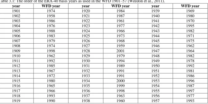
10 reanalyses (NCEP-DOE Reanalysis 2 for the baseline simulations) at 3-hour intervals (Dirmeyer et al., 2006). The reanalysis data was hybridized with observational data, and corrected for differences in elevation between the reanalysis model topography and the ISLSCP Initiative II mean topography. Recently Weedon et al. (2010, 2011) created a consistent meteorological forcing data for hydrological studies used to force LSMs and GHMs, the WATCH Forcing Data (WFD). Creation of WFD precipitation (rainfall and snowfall) is described in this chapter. Construction of WFD data involves two steps: interpolation of the ECMWF Re-Analysis to a grid of 0.5ºx0.5º and correction of reanalysis with the observationally based data. Variables in meteorological data are divided in two types: state variables (near-surface air temperature, specific humidity, wind speed and surface pressure) and flux fields (radiation and precipitation). The WFD was derived from the surface variables of the 40 years European Centre for Medium-Range Weather Forecasts (ECMWF) Re-Analysis (ERA-40) (Uppala et al. 2005) for the period 1958 to 2001, but from reshuffled ERA-40 data for the period 1901 to 1957 (Table 3.1). The WFD consist of subdaily, gridded, half-degree resolution, meteorological forcing data. Variables included are (i) wind speed at 10 m, (ii) air temperature at 2 m, (iii) surface pressure, (iv) specific humidity at 2 m, (v) downward longwave radiation flux, (vi) downward shortwave radiation flux, (vii) rainfall rate, and (viii) snowfall rate. Meteorological data was produced at both daily and subdaily time steps: flux fields are provided 3-hourly, while state variables are 6-hourly. These global data are stored at 67 420 points over land (excluding Antarctica). Data is available as WFD-land-longitude-latitude-z files either in NetCDF or DAT formats.
ERA-40 data was interpolated to ½º resolution on the CRU land mask, adjusted for elevation changes where needed, and bias corrected using monthly observations. The main procedures described by Ngo-Duc et al. (2005) and Sheffield et al. (2006) were adopted to generate the WFD. Temperature, surface pressure, specific humidity, and downward longwave radiation were adjusted sequentially in that order because they are interdependent via the elevation adjustment. Diurnal air temperature was bias corrected with CRU data (New et al., 1999, 2000; Mitchell and Jones, 2005). Shortwave downward radiation (SWdown) was corrected using CRU cloud cover fractions, having found the grid point-specific correlations between monthly average SWdown and ERA-40 cloud fraction. SWdown was also adjusted in clear sky and cloudy sky for the effects of tropospheric and stratospheric aerosol loading. ERA-40 precipitation output consists of both rainfall and snowfall (Betts and Beljaars, 2003), and the convective and large-scale precipitation are added to produce the total precipitation. The most serious problem diagnosed in the ERA-40 analyses is excessive tropical oceanic precipitation in later years, particularly in stream 1 after 1991 (Troccoli and Kallberg, 2004). To avoid these problems precipitation was adjusted using both a wet days correction from CRU and precipitation totals from the GPCCv4 full data product (Rudolf and Schneider 2005; Schneider et al. 2008; Fuchs 2009), and corrected for undercatch (snowfall and rainfall separately) based on Adam and Lettenmaier (2003). Observation based datasets are used to spatially downscale the reanalysis, which is available at high temporal resolution, and at the same time remove biases in the reanalysis.
In the next section WFD precipitation (rainfall and snowfall rate) is described; for more detailed information of state and radiation variables see Weedon et al. (2010, 2011).
2.2 Correction for rainfall and snowfall rate
WFD precipitation is produced by carrying out a set of empirical corrections to precipitation of reanalysis and observations. The reanalysis systematic errors are removed via a multiplicative scaling factor that is based on the ratio of observed monthly rainfall to reanalysis estimates. The generation of precipitation data involved six steps: 1) bilinear interpolation, 2) combining rainfall and snowfall totals while retaining the rainfall/snowfall ratio for each location and time step, 3) adjusting the number of “wet” (i.e., rain or snow) days per month to match the CRU TS2.1 observations, 4) adjusting the monthly precipitation totals to match GPCCv4 precipitation (or CRU precipitation), 5) reassigning the precipitation into rain and snow using the original ratio, and 6) adjusting the monthly totals using gridded average precipitation gauge correction (separately for rainfall and snowfall).
Chapter 2 - The land surface model and forcing data in the presence of reanalysis CRU and GPCC observation based data, were used for correcting systematic errors, in particular reduction of the number of wet days covering global land areas at monthly resolution. CRU data is a set of mean monthly surface climate data over global land areas, excluding Antarctica, for nearly all of the twentieth century. The data set is gridded at 0.5 degree latitude/longitude resolution and includes seven variables: precipitation, mean temperature, diurnal temperature range, wet day’s frequency, vapour pressure, cloud cover, and ground-frost frequency (New et al., 2000; Mitchell and Jones, 2005). All variables have mean monthly values for the period 1901-2001 (TS2.1 version). The Global Precipitation Climatology Project (GPCP), presented in this chapter, has produced and released monthly mean estimates of precipitation on a 0.5º lat × 0.5º lon grid for the period 1901-2001 (GPCCv4). GPCC precipitation is a combination of gauge observations with satellite estimates and includes estimates of uncertainty for each location and month.
2.2.1 Wet days correction
Betts et al. (2003a, 2003b), Hagemann et al. (2005) and Uppala et al. (2005) found disparities between ERA-40 monthly precipitation total and both CRU and GPCC totals. Due to the presence of too many wet days (number of days per month with rainfall/snowfall) in the tropics (Betts and Beljaars, 2003; Hagemann et al., 2005; Uppala et al., 2005), a wet days correction has been adopted. Figure 2.1 compares the zonal average of ERA-40 precipitation (dashed blue line) before bilinear interpolation and wet days correction with observational zonal average from CRU (TS 2.1 and TS 3.1) and GPCC (v4 and v6) from 1958 to 2001. ERA-40 precipitation is overestimated in the tropics over land compared to GPCC and CRU data. In the mid-latitudes ERA-40 patterns (not shown) are similar to observations. The need for a wet day correction is evident in the mid-latitudes.
Figure 2.1: Zonal average of precipitation for the ERA-40 period (1958 to 2001), only land points.
The method adopted for wet days correction is the main difference in the derivation of previous precipitation forcing datasets. Ngo-Duc et al. (2005), for example, did not correct wet days, whereas Sheffield et al. (2006) used a statistical correction (Sheffield et al. 2004) that was designed to cope with spurious standing wavelike patterns in the high northern-latitude wet days characteristics of the NCAR– NCEP data. However, the Sheffield et al. (2004) correction meant that spatial continuity of individual precipitation events was sometimes compromised (see Fig. 7 of Sheffield et al., 2004), and it also required the adjustment of several associated variables when wet days were ‘‘created’’ to match the CRU data. Additionally, Sheffield et al. (2006) introduced the correction of number of CRU wet days as well as correction of precipitation gauge-undercatch via the gridded average catch ratios of Adam and Lettemaier (2003).
Chapter 2 - The land surface model and forcing data in the presence of reanalysis
12
2.2.2 Monthly bias correction
Figure 2.2 and Figure 2.6 show time series of global and land average precipitation for: the CRU (TS 2.1 and TS 3.1); GPCC (v4 and v5) datasets (only WFD land-mask) and ERA-40 or WFD precipitation (CRU and GPCC version) before and after corrections. The ERA40 dataset is biased by 42 mm/month over global land areas excluding Antarctica. Errors in the ERA reanalysis precipitation at monthly scales translate into errors in land surface fields like evapotranspiration, soil moisture, and snow cover (Sheffield et al., 2004). Ngo-Duc et al. (2005a) investigated the effect of precipitation bias on runoff generation. These biases contributed for larger errors in resultant large basin river discharge than biases in air temperature and radiation.
Figure 2.2: Running average (annual) of precipitation over continental area excluding Antarctica for CRU, GPCC and ERA-40 datasets. ERA-ERA-40 is discretized here at 1ºx1º grid.
Information on the precipitation averaged over land, for each of the three decades is shown in Table 2.1. From the 70s onwards, a succession of satellite-borne instruments and the increasing numbers of observations from aircraft, ocean-buoys and other surface platforms, provided assimilable data; however there was a declining number of radiosonde ascents (Uppala et al., 2005). In order to cover the entire ERA-40 period, the first and last column in the table represent 13 and 11 years, respectively. ERA-40 results (based on 3h, and 1ºx1º data) are compared with global observations (CRU and GPCC monthly data). There is an increase in ERA40 average precipitation from 60s to 70s decades. There are no satellite data available for assimilation until 1961. In the observational datasets for the various periods the average precipitation is about 69 mm/month.
Table 2.1: Global precipitation over land for the years 1958-70, 1971-80, 1981-90 and 1991-2001, in mm per month, from the reanalysis performed at ECMWF (ERA-40) and from other data sources: CRU (TS 2.1 and TS 3.1) and GPCC (v4 and v6). Antarctica is excluded. Period Decade 60s 1958-70 Decade 70s 1971-80 Decade 80s 1981-90 Decade 90s 1991-01 ERA-40 (land, 1ºx1º) 69 81 80 79 CRU TS2.1 69 70 69 69 CRU TS3.1 69 70 68 70 GPCCv4 69 70 69 69 GPCCv6 69 70 68 69
A bias correction procedure was implemented to minimize the discrepancies between the monthly observations and reanalysis. The monthly bias correction was applied to the reanalysis data (after bilinear interpolation and wet-days correction) so that the mean monthly values match those from GPCCv4 and CRU monthly precipitation, respectively. To remove the bias in the reanalysis the 3-hourly, after wet-days correction, values are scaled so that their monthly totals match those the GPCC dataset (Ngo-Duc et al., 2005a, Sheffield et al., 2006 and Weedon et al., 2010, 2011):
PERA,3h∗ = Pobs,mon
PERA,mon× PERA,3h (2.1)
where the asterisk indicates a corrected value and the subscripts indicate the data source (observations and reanalysis) and the temporal resolution (3 hourly or monthly). Observations have been obtained from the Global Precipitation Climatology Centre half-degree version 4 full product (GPCC v4). This consists of monthly gridded precipitation totals from rain-gauge observations For some places, especially islands, represented by one or very few boxes in the CRU grid that are not covered by GPCC v4, we have employed the CRU TS2.1 precipitations totals. A similar bias correction was applied using CRU TS2.1 precipitation totals.
Chapter 2 - The land surface model and forcing data in the presence of reanalysis In a small number of grid boxes and some months, precipitation rates are close to zero. The monthly bias correction then had the effect of increasing these rates such as to imply there was spurious background drizzle between more normal precipitation events. In semiarid areas this is inconsistent with local climatic conditions but, fortunately from the point of view of hydrological modelling, this spurious low-level background precipitation is not significant. When there were too few wet days in interpolated ERA-40, for the (very few) locations, the adjustment of monthly precipitation totals sometimes implied high precipitation rates. These “outliers” rates were limited to a rate corresponding to the 99.999 % lognormal probability precipitation rate for the relevant calendar month and grid box (Weedon et al., 2010, 2011).
2.2.3 Maximum precipitation: outliers
The statistical characterization of precipitation is useful in understanding the large-scale space and time variability of the process and is helpful in assessing the accuracy of the precipitation retrievals by imposing constraints that must be satisfied by the spatial and temporal averages of the reanalysis or observations. One topic of interest is the probability density function (PDF) of precipitation rates. This PDF is indispensable and particularly so when it comes to the estimation of the maximum of precipitation that occurred at single location. The PDF of precipitation rate over large areas is fairly stable over time and space (Meneghi and Jones, 1993), for this reason, the parameters of the particular distribution can be used for representing very different climatological conditions (Wilks, 1995). The lognormal distribution, as well as the gamma distribution, is commonly used to represent precipitation rates. The lognormal distribution assumes that the logarithms of the data are normally distributed. Cho et al. (2004) analysed the spatial characteristics of nonzero rain rates to develop a PDF model of precipitation using satellite rainfall data. The lognormal distribution overestimates the sample mean, whereas the gamma distribution underestimates it. These differences are caused by the inflated tail in the lognormal distribution and the small shape parameter in the gamma distribution. The gamma fits outperformed the lognormal fits in rainy regions, while the lognormal fits were better than the gamma fits in dry regions (Cho et al., 2004). To avoid extreme values, also known as outliers, in our data we fitted a lognormal distribution at the probability of 99.999 %.
Considering the ECMWF’s reanalysis (ERA-40 and, recently, ERA-interim), the properties of precipitation were investigated, characterizing the PDF of precipitation rates. At each WFD land point (½ degree) the lognormal distribution was fitted and the maximum of precipitation rate was calculated based on the parameters of the distribution. No-rain data (i.e., P = 0) are included to avoid overestimating mean rain rates.
Three standard techniques for fitting a theoretical PDF to data are the method of moments, the maximum likelihood method, and the minimum χ2 method. The methods of moments use the sample mean and variance as the mean and variance of the fitted distribution. Although inefficient (Wilks, 1995) we used this method due to deadline limitations.
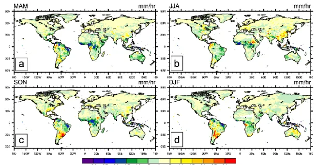
Maximum of precipitation is concentrated over tropical zone in the intertropical convergence zone and monsoon areas. The highest precipitation occurs over South America and Eastern America (over than 50 mm per hour). Figure 2.3 shows differences between the seasonal average of maximum precipitation of ERA-I and ERA-40. Positive differences (yellow to red in pictures) indicate that maximum of
Chapter 2 - The land surface model and forcing data in the presence of reanalysis
14 Figure 2.3: Differences between max ERA-I and ERA-40 maximum of precipitation. For each location and month, the 99.999% percentile was computed (see text); each seasonal panel represents averaged values of respective monthly 99.999% percentiles.
2.2.4 Correction for gauge undercatch
Adam and Lettenmaier (2003) developed gridded mean monthly catch ratios (CRs) for adjustment of wind-induced undercatch and wetting losses for global gridded precipitation products. The precipitation gauge correction used separate average calendar monthly catch ratios for rainfall and snowfall rates at each half-degree grid box. No attempt was made to adjust precipitation rates to allow for effects of orography (Adam et al., 2006).
The seasonally averaged spatial distribution of 0.5º global correction ratios of rainfall (RainCR) and snowfall (SnowCR) are shown in Figure 2.4 and Figure 2.5, respectively. These correction ratios were applied to the 3-hourly ERA-40 after wet days and bias corrections. In general, the CRs increase from north to south with lower values in high-altitude regions and in high wind speeds (Adam and Lettenmaier, 2003). Seasonal CRs are smaller than 1, about 0.8, causing a slightly increase of rainfall, except in the Canadian Rockies during the cold season (see Figure 2.4a). Positive values of catch rations that only happens in the Canadian Rockies during DJF, can reach 1.2, reduce more than 83 % the original rainfall.
Figure 2.4: Seasonally averaged gauge catch ratios for rain, RainCR, from Adam and Lettenmaier (2003). Values larger (smaller) than 1 decrease (increase) ERA-40 rainfall. Corrected Rainf = Rainf/RainCR
Chapter 2 - The land surface model and forcing data in the presence of reanalysis These bias adjustment methodology applied to snowfall rate results in a slight increase in snowfall (see Figure 2.5). Blue and green values indicate an increase of snowfall, as rainfall. Over the Canadian Rockies during the warm season, CRs correction will reduce winter snowfall (correction ratios are about 1.1). In South Hemisphere and some location in North Hemisphere (e.g. Iberian Peninsula) there are no snowfall correction.
Figure 2.5: Seasonally averaged gauge catch ratios for snow, SnowCR, from Adam and Lettenmaier (2003). Values larger (smaller) than 1 decrease (increase) ERA-40 snowfall. Corrected Snowf = Snowf/SnowCR.
The running average of precipitation over continental area for WFD and observed precipitation are presented in Figure 2.6. The global average reflects the inter-annual variability of the observations, but the average amount is slightly higher than the observed result of subsequent corrections to bias elimination.
Chapter 2 - The land surface model and forcing data in the presence of reanalysis
16
2.3 Land Surface Model – HTESSEL and CTESSEL
The land surface model TESSEL (Tiled ECMWF Scheme for Surface Exchanges over Land) was the land surface scheme used by ERA-40. It is a one-dimensional model with four levels of prediction for the soil temperature and water content, and free drainage zero heat flux lower boundary condition. The land surface scheme includes up to six coexisting land surface tiles (bare ground, low and high vegetation, intercepted water and shaded and exposed snow). Soil freezing is parameterized according to Viterbo et al. (1999), while soil water and energy transfers are described in Viterbo and Beljaars (1995), with significant model upgrades, developed for ERA40, are described in van den Hurk et al. (2000). Revisions concerning the snow and the soil hydrology, labelled as HTESSEL, are detailed by Dutra et al. (2010) and Balsamo et al. (2011a, 2011b), respectively. The carbon enabled version, CTESSEL (Boussetta et al., 2013), is described in 2.3.4.
Figure 2.7: Schematic representation of the structure of (a) TESSEL land-surface scheme and (b) spatial structure added in H-TESSEL. For a given precipitation, P1=P2 the
scheme distributes the water as surface runoff, R, and drainage, D, with functional dependencies on orography, σ, and soil texture, respectively. (Balsamo et al., 2009).
2.3.1 TESSEL hydrology
The TESSEL scheme is shown schematically in Figure 2.7a. The scheme includes up to six land surface tiles (bare ground, low and high vegetation, intercepted water and shaded and exposed snow) and two over water (open and frozen water), with separate surface energy and water balances. It considers a four-layer soil. The depths are chosen in an approximate geometric relation: 7 cm for the top four-layer, 21 cm, 72 cm and 189 cm. These four layers are enough for representing correctly all time-scales from one day to one year. The soil can be covered by a single layer snow. In each grid box, two vegetation types are present: a high and a low vegetation type.
2.3.1.1 Soil heat budget
The soil heat transfer is assumed to obey the Fourier law of diffusion: (ρC)s ∂T ∂t = ∂ ∂z(λT ∂T ∂z) + 𝐿𝑓𝜌𝑤 𝜕𝜃𝐼 𝜕𝑡 (2.2)
where (ρC)s is the volumetric soil heat capacity [J m−3K−1], T is the soil temperature [K], z is the
vertical coordinate in m, λT is the thermal conductivity [W m−1K−1], Lf is the latent heat of fusion [Jkg−1], ρ
w is the water density [kgm−3], and θI is the ice water contents [m3m−3]. The heat fluxes are
predominantly in the vertical direction. The second term of r.h.s of the equation represents the thermal effects of phase changes, of relevance in cold environments; they are described in detail in Viterbo et al. (1999).
Boundary conditions for the energy equation (2.2) are a net heat flux at the surface (sum of the radiative, latent and sensible heat fluxes) and a zero flux at the bottom.


![Figure 4.10: Simulated annual cycle over land computed from [1971-2000] of the zonal precipitation (left), evapotranspiration (middle) and runoff (right): LPJmL, MacPDM, MPI-HM, WaterGAP, VIC, and HTESSEL](https://thumb-eu.123doks.com/thumbv2/123dok_br/18555945.906323/61.893.110.785.96.513/figure-simulated-computed-precipitation-evapotranspiration-macpdm-watergap-htessel.webp)