Improving airflow and thermal distribution in a real data centre room through Computational Fluid Dynamics modeling

Improving Airflow and Thermal Distribution in a Real Data Centre Room through

Computational Fluid Dynamics Modeling

Diogo G.C.S. Macedo

, Pedro D. Gaspar

, Pedro D. Silva

, Miguel T. Covas

, Radu Godina

ALTICE/MEO - Serviços de Comunicações e Multimédia, SA, Quinta Grila DATACENTER, 6200-292 Covilhã, Portugal; 4 _{Research and Development Unit in Mechanical and Industrial Engineering (UNIDEMI), Department of Mechanical and} Industrial Engineering, Faculty of Science and Technology (FCT), New University of Lisbon, 2829-516 Caparica, Portugal;

e-mail: [email protected] & [email protected]

Abstract—A Data Centre is a physical space that groups

together computer equipment such as servers, storage arrays, among other equipment. It can be used for storage, processing and data protection. The majority of data centres operate 24 hours a day, and must provide the user with guarantees in terms of security and performance. Energy consumption is therefore permanent and the level of assistance and maintenance high. Data Centres have an ecological impact that is almost invisible to many users. In this paper a computational fluid dynamics (CFD) model of the airflow and thermal distribution of a real data centre room with 208 racks is proposed. Two case studies are presented and simulated with a high thermal load subjected to the minimum and maximum air flow velocity, respectively. The objective is to assess if the computer room air conditioning unit (CRAC) can cool the racks of the data centre in order to efficiently refrigerate all the hot spots.

Keywords-hot spots; data centre; computational fluid dynamics; air-conditioning systems; computer room air conditioning; energy efficiency

I. INTRODUCTION

Data centres were responsible for 1.12–1.5% of the entire electricity consumption in the world in 2010 [1] and in 2013 the electricity consumption in the world of the information technology (IT) sector represented as much as 10% [2]. Energy consumption is a major expense factor for data centres, which must combine the demanding activity of their servers with their data management and optimization of their energy consumption [3].

Optimizing data centre power consumption is high on the priority list of data centre managers. However, it continues to reveal challenges given the increasing percentage of ongoing costs that this consumption represents [4]. For instance, the ventilation and cooling system absorbs almost 40% of the overall energy consumption in a data centre [5], since the majority of the energy consumed by the data centre equipment is converted into heat [6]. Additionally, the stakes are very high for data centre managers. Several researchers and policy makers have put a spotlight on the carbon footprint of the IT organizations and their data centres [7]. Operators had to adapt and reveal to the general public their energy consumption, their method of cooling, and more generally, the very conception of their layout and architecture [8].

That is why the great interest and importance of the personnel in charge of the data centre operation to take necessary measures to reduce the energy consumption, costs, CO2 emissions, and on the other hand, to enhance the efficiency and performance of data centres with fewer resources in order to achieve the correct efficiency of the equipment [9]. One method to achieve this is to use computational fluid dynamics (CFD) tools.

CFD has become a widespread, robust and useful tool in the analysis of systems of practical interest, namely the physical and chemical phenomena involved in fluids mechanics with heat transfer such as mass, momentum, energy conservation [10]. Such tool has become so popular due to the fact that the computational resources have been gradually increasing in capacity, memory and speed. Also, their cost has been drastically decreasing over time [11].

Several researchers have used CFD to model data centres and predict properties distributions. In [12] a CFD analysis of temperature, airflow and pressure distribution of a data centre with two racks and located at Central Queensland University, Australia was developed. This study identified the potential high temperature area within the rack. The researchers in [13] use CFD to investigate the airflow pattern for a common data centre with under-floor air supply system and found that the computer room air conditioning unit (CRAC) can be optimized. A fan-assisted cooling was proposed in [14] within open and contained raised-floor data centres by using CFD in order to optimize the energy efficiency. A CFD simulation was used in [15] to identify which of the proposed three airflow patterns for a common data centre is the most efficient. An optimization technique was recommended in order to overcome the deficiencies in cooling system at the rack level. A literature review of several cooling systems for data centres was developed in [16] and CFD simulations were made for each category of these systems. A numerical simulation using CFD to predict the temperature and air flow distribution of a small data centre in order to reach an optimal thermal control was proposed in [17].

In this study, a CFD model of the airflow and thermal distribution of a real data centre room with 208 racks is proposed. The location of this data centre is a small European city. Two case studies are presented and simulated with a large thermal load subjected to the minimum and maximum air flow velocity, respectively. The aim is to assess whether the computer room air conditioning unit

(CRAC) can cool the racks of the data centre with the purpose of efficiently removing all the identified hot spots. In both case studies the thermal load is 75% of the maximum capacity of the heat flow limit condition. The tool used to simulate and study the airflow in the room is the ANSYS™ Fluent package.

This paper is organized as follows. The proposed model description can be found in section 2. In section 3 the results of both case studies are depicted and analysed. Conclusions are drawn in section 4.

II. METHODOLOGY

The conservation laws for mass momentum and energy are generally the governing equations of fluid flows. The Reynolds number is usually quite high in the majority of data centre rooms. Thus, in cases in which simulations of the airflow are needed, a turbulence must be considered [18]. The k–ε model is the turbulence model commonly utilized in similar simulation studies of data centres’ airflow [19].

The study in this paper is based on the governing equations from [20]. The model was created in a manner in which the room is entirely isolated and the influence of heat transfer from the exterior is ignored (external thermal radiation and convection modes are neglected as well as thermal conduction through the walls). Therefore, the walls of the room in this model are adiabatic.

The continuity, momentum and , turbulence (standard k-ε model) equations employed in this paper rely on equations from [20] and [21], usual for this purpose. The equations that represent the model are as follows:





 

t k

k

div Uk div grad k P

t   _{  }              _{  } (1)





 

div U div grad

t C P C k k      _{   }   _     _{   }     _{  }   (2)

In which k represents the turbulent kinetic energy in (m2/s2), U is the velocity vector (m/s), μT is the turbulent

viscosity (kg/m.s), the Prandtl number for turbulent kinetic energy is given by σk, the turbulent energy production is

given by [kg/(m.s3)], ε is the turbulent energy dissipation, the Prandtl number for turbulent energy dissipation is represented by σε, C1ε is the production constant and C2ε is

the dissipation constant.

Constants σε, σk, C2ε, Cμ, and C1ε, are set to values 1.3, 1,

1.92, 0.09 and 1.44 respectively, as in [21].

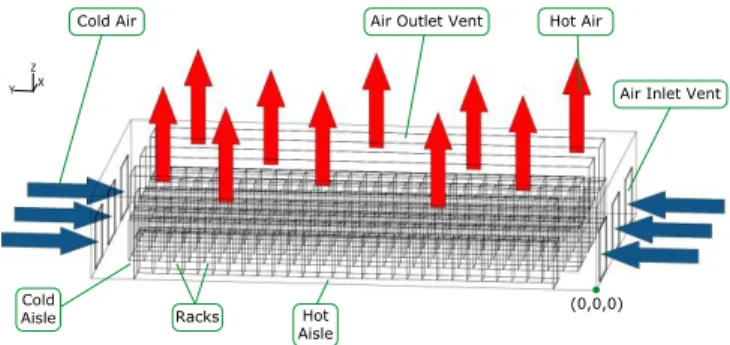
ANSYS™ Fluent was the CFD tool used to develop the studied model. Initially, a three-dimensional (3D) geometry model of the data centre room was developed. The 3D geometry was created with the aid of computer-aided design (CAD) tools and exported to ANSYS™ Fluent. In this case, the 3D geometry was simplified in order to avoid a case in which the mesh generated by the ANSYS™ Fluent package is very computational demanding or overwhelming. Thus, the racks are presented as parallelepipeds. Fig. 1 shows the proposed 3D geometry for this study.

Racks

Air Outlet Vent

Air Inlet Vent

Cold Air Hot Air

Cold Aisle Hot Aisle Y Z X (0,0,0)

Figure 1. A 3D representation of the studied data centre room.

To consider the control volume formulation, a mesh of the geometry was created. A good quality mesh is essential for this study so that the numerical solution could converge and the obtained results could be more reliable. The mesh created for this study is made of hexahedral elements, such as the racks and the hot aisles and tetrahedral elements, such as the cold aisles. Employing only tetrahedral elements would have meant a more complex mesh, which would have been a better option, but more demanding for the workstation. The mesh is characterized by 2 341 172 control volumes, 1 183 613 nodes. The mesh quality was assessed by the Aspect Ratio and skewness, 1.645 and 0.177, respectively. Such values required a high computational capacity from the workstation.

A. Boundary conditions

The boundary conditions that are used in simulations are based on the data obtained from the data centre. The pressure loss in the racks was taken from [22], where it is defined a pressure loss of 7.5 Pa for a flow going through a 80% perforated plate.

The air is the fluid considered for the simulation and it’s assumed to be incompressible, signifying that the values shown in Table 1 are constant. A dimensionless temperature of 7.09×10-4 was used to characterize the fluid zone. Only in cases in which all the residuals achieve the iterative process stop criterion λ = 1 × 10-3 for every variable, the solution is considered convergent, while the stop criterion of λ = 1×10-6 is only used for the variable energy. The relaxation factors are the ones given by ANSYS™ Fluent software package by default.

The number of iterations for all the simulations was set to the fixed value of 1500. The reason for such a high number is that desired solutions did not achieve the stop criterion λ. Nevertheless, 1500 iterations are more than enough to reach the possible convergence of the solution since in this model every variable stabilized significantly earlier than the last iteration.

TABLE I. THE AIR’S ATMOSPHERIC PROPERTIES IN THE ROOM.

Constants Values

Specific Heat Cp = 1006,14 J/kg.K

Specific Mass ρ = 1,21 kg/m3

Thermal Conductivity k = 0,0256706 W/m._K

The heat transfer was considered to be uniform on the surface of the racks and on the external wall. The impact air leakage or personnel movement was also ignored for this study.

III. ANALYSIS AND DISCUSSION OF RESULTS

In the first case study addressed in this study, 75% of the thermal load of the heat flow limit condition is modelled and studied for the minimum and maximum air flow velocity. The boundary conditions considered for this case study are the following: 75% of the maximum thermal load generated by the racks: qadm = 0.750 and the minimum air flow

dimensionless velocity: vadm = 0.

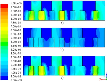
The temperature field predictions are shown in Figs. 2, 3 and 4 of the x, y and z planes, respectively.

Several hot spots are predicted at the extremity of all rack lines, as depicted in Figs. 2, 3 and 4. The hot spots can be identified by detecting colours associated to values superior to dimensionless temperature equal to 0.350 on the left scale. By observing Fig. 4a), higher heat intensity at the bottom of the racks is predicted and can be observed. The air flow is insufficient in this region of the room. The reason is that the intensity of the airflow is stronger in the middle of the air vents.

Also, by observing Fig. 2b) it is possible to confirm that the first line of racks, the top line in Fig. 1, is shorter than the remaining lines, thus meaning that even though the racks located at the extremities show a probability of occurrence of hot spots, only two from each side aren’t properly cooled when compared with Figs. 2c) and 2e).

Figure 2. Dimensionless temperature field in the y-z plane with the planes a) xadm = 0.042, b) xadm = 0.116, c) xadm = 0.526, d) xadm = 0.589, e) xadm =

0.779 and f) xadm = 0.842.

Figure 4 shows that for 75% of the maximum load and for a minimum air flow velocity, hot spots occur at the end of the every rack row and in the extraction zone.

The boundary conditions in the second case study are defined as by vadm being equal to 1 and qadm being 0.750. The

temperature field predictions are shown in Figs. 5, 6 and 7 of the x, y and z planes, respectively.

Figure 3. Dimensionless temperature field in the x-z plane with the planes a) yadm = 0.100, b) yadm = 0.485 and c) yadm = 0.900.

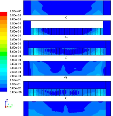
Figure 4. Dimensionless temperature field in the x-y plane with the planes a) zadm = 0, b) zadm = 0.244, c) zadm = 0.489, d) zadm = 1.

The analysis of Figs. 5, 6 and 7 allow predicting that no hot spots are formed. This happens because the air flow velocity is at the highest level, meaning that the CRAC units are capable to successfully exhaust the hot air.

Figure 5. Dimensionless temperature fields in the y-z plane with the planes a) xadm = 0.042, b) xadm = 0.116, c) xadm = 0.526, d) xadm = 0.589, e) xadm =

0.779 and f) xadm = 0.842.

Figure 6. Dimensionless temperature fields in the x-y plane with the planes a) zadm = 0, b) zadm = 0.244, c) zadm = 0.489, d) zadm = 1.

Even in this case it is possible to observe that the warmer air is near the extremities of the lines of racks. As in the previous case, Figs. 6 and 7 confirm that the heat is more intense at the bottom of the racks and closer to extremities. This air located at the end of the racks’ lines is warmer due to the same reason as in the first case. The velocity vectors are depicted in Figs. 8a) and 8c), where it can be noticed that the airflow in the mentioned positions is imperfect. On the other hand, the air flows correctly in the middle of the room, as shown in Fig. 8b). The validation of the numerical model is made through measurements given by the data centre management.

The air flow is not optimal near the extremities of the lines of the racks. This happens due to the fact that the room has an imperfect layout.

Figure 7. Dimensionless temperature fields in the x-z plane with the planes a) yadm = 0.100, b) yadm = 0.485 and c) yadm = 0.900.

Figure 8. Dimensionless velocity vectors for the x-y plane a) yadm = 0.000,

The flawed cooling mentioned above can be observed the zoomed section of Fig. 8c), where the air flows poorly to the cold aisle from the hot aisle. However, as confirmed by Figs. 2-7, in the middle of the room the cooling is much more efficient, as evidenced by the air flow represented in Fig. 8b), in which the air flows correctly to the cold aisle from the hot aisle.

As mentioned in Section 2, the maximum thermal load is 75%, which is not usual for the data centre and occurs when the demand is higher and the majority of racks operate. However, even if in these cases the CRAC units can refrigerate the room, the refrigeration is achieved by consuming a high quantity of energy. Thus, instead of upgrading the CRAC units, which is costly, a solution could be altering the layout of the data centre room and trying to optimize it in order to efficiently cool the racks. One solution could be removing a few racks and thus being able to avoid any hot spot by reducing the air flow velocity.

IV. CONCLUSIONS

A parametric study using CFD modelling tools for a data centre room operating with 208 racks was proposed in this paper with the intention of studying the airflow. A 75% of the maximum thermal load was used in this study, which is a high number for the data centre, thus not occurring very often. Simulations are made for the heat flow limit condition and two case studies are analysed for the minimum and maximum air flow velocity. The results predict that in the case of the minimum air flow velocity several hot spots appear. The results also indicate that in the case of the maximum air flow velocity all the racks are cooled, providing hot spots removal. However, cooling in this manner consumes a high amount of energy. All the hot spots are located at the extremities of the aisles and this occurs due to the deficient cooling of the room due to the inadequate location of the CRAC units. This occurs on both case studies. Thus, even though all the racks are successfully cooled with a maximum air flow velocity, this solution is not the best. The imperfect airflow observed at the extremities of the aisles happens due to a flawed layout of the data centre room. One way to diminish the air flow velocity and avoiding the occurrence of hot spots could be withdrawing a few racks from the extremities of the lines. This will allow for an improved airflow in the room.

ACKNOWLEDGMENT

The current study was funded in part by Fundação para a Ciência e Tecnologia (FCT), under project UID/EMS/00151/2013 C-MAST, with reference POCI-01-0145-FEDER-007718. Radu Godina would like to acknowledge the financial support from Fundação para a Ciência e Tecnologia (FCT), (grant UID/EMS/00667/2013).

REFERENCES

[1] S.-W. Ham, M.-H. Kim, B.-N. Choi, and J.-W. Jeong, “Simplified server model to simulate data center cooling energy consumption,”

Energy Build., vol. 86, pp. 328–339, Jan. 2015.

[2] M. Wahlroos, M. Pärssinen, S. Rinne, S. Syri, and J. Manner, “Future views on waste heat utilization – Case of data centers in Northern Europe,” Renew. Sustain. Energy Rev., vol. 82, pp. 1749–1764, Feb. 2018.

[3] “Data cooling centre goes green,” World Pumps, vol. 2017, no. 2, pp. 28–29, Feb. 2017.

[4] C. Nadjahi, H. Louahlia, and S. Lemasson, “A review of thermal management and innovative cooling strategies for data center,”

Sustain. Comput. Inform. Syst., vol. 19, pp. 14–28, Sep. 2018.

[5] X. Zhang, T. Lindberg, N. Xiong, V. Vyatkin, and A. Mousavi, “Cooling Energy Consumption Investigation of Data Center IT Room with Vertical Placed Server,” Energy Procedia, vol. 105, pp. 2047– 2052, May 2017.

[6] B. Lajevardi, K. R. Haapala, and J. F. Junker, “Real-time monitoring and evaluation of energy efficiency and thermal management of data centers,” J. Manuf. Syst., vol. 37, pp. 511–516, Oct. 2015.

[7] L. Grange, G. Da Costa, and P. Stolf, “Green IT scheduling for data center powered with renewable energy,” Future Gener. Comput.

Syst., vol. 86, pp. 99–120, Sep. 2018.

[8] H. Rong, H. Zhang, S. Xiao, C. Li, and C. Hu, “Optimizing energy consumption for data centers,” Renew. Sustain. Energy Rev., vol. 58, pp. 674–691, May 2016.

[9] M. Sharma, K. Arunachalam, and D. Sharma, “Analyzing the Data Center Efficiency by Using PUE to Make Data Centers More Energy Efficient by Reducing the Electrical Consumption and Exploring New Strategies,” Procedia Comput. Sci., vol. 48, pp. 142–148, Jan. 2015.

[10] “Application of Computational Fluid Dynamics to Ventilation System Design,” in Ventilation for Control of the Work Environment, John Wiley & Sons, Ltd, 2004, pp. 374–390.

[11] J. Tu, G.-H. Yeoh, and C. Liu, “Chapter 1 - Introduction,” in

Computational Fluid Dynamics (Third Edition), J. Tu, G.-H. Yeoh,

and C. Liu, Eds. Butterworth-Heinemann, 2018, pp. 1–31.

[12] N. M. S. Hassan, M. M. K. Khan, and M. G. Rasul, “Temperature Monitoring and CFD Analysis of Data Centre,” Procedia Eng., vol. 56, pp. 551–559, Jan. 2013.

[13] C. Gao, Z. Yu, and J. Wu, “Investigation of Airflow Pattern of a Typical Data Center by CFD Simulation,” Energy Procedia, vol. 78, pp. 2687–2693, Nov. 2015.

[14] Z. Song, “Studying the fan-assisted cooling using the Taguchi approach in open and closed data centers,” Int. J. Heat Mass Transf., vol. 111, pp. 593–601, Aug. 2017.

[15] Z. Huang, K. Dong, Q. Sun, L. Su, and T. Liu, “Numerical Simulation and Comparative Analysis of Different Airflow Distributions in Data Centers,” Procedia Eng., vol. 205, pp. 2378– 2385, Jan. 2017.

[16] B. Watson and V. K. Venkiteswaran, “Universal Cooling of Data Centres: A CFD Analysis,” Energy Procedia, vol. 142, pp. 2711– 2720, Dec. 2017.

[17] C. Zhou, C. Yang, C. Wang, and X. Zhang, “Numerical simulation on a thermal management system for a small data center,” Int. J. Heat

Mass Transf., vol. 124, pp. 677–692, Sep. 2018.

[18] E. Wibron, A.-L. Ljung, and T. S. Lundström, “Computational Fluid Dynamics Modeling and Validating Experiments of Airflow in a Data Center,” Energies, vol. 11, no. 3, p. 644, Mar. 2018.

[19] Y. Fulpagare and A. Bhargav, “Advances in data center thermal management,” Renew. Sustain. Energy Rev., vol. 43, pp. 981–996, Mar. 2015.

[20] J. Ni, B. Jin, B. Zhang, and X. Wang, “Simulation of Thermal Distribution and Airflow for Efficient Energy Consumption in a Small Data Centers,” Sustainability, vol. 9, no. 4, p. 664, Apr. 2017. [21] M. L. Hoang, P. Verboven, J. De Baerdemaeker, and B. M. Nicola ,

“Analysis of the air flow in a cold store by means of computational fluid dynamics,” Int. J. Refrig., vol. 23, no. 2, pp. 127–140, Mar. 2000. [22] T. North, “Understanding How Cabinet Door Perforation Impacts