A comparison between geometric properties and central moments to detect P300 waves

(1)

2018

UNIVERSIDADE DE LISBOA FACULDADE DE CIÊNCIAS DEPARTAMENTO DE INFORMÁTICA

A Comparison Between Geometric Properties and Central

Moments to Detect P300 Waves

João Ricardo Dias Cardoso

Mestrado em Informática

Dissertação orientada por:

(2)

(3)

Acknowledgments

My first acknowledgement will be to my supervisor Manuel Jo˜ao Caneira Monteiro da Fonseca who helped me a lot with this work which would have been impossible to accomplish without him. I recognize that he also suffered a lot with me because I am not organized and I am a terrible writer, which lead him to spend blank nights correcting my writable mistakes. I can only thank him everyday for helping me. I also want to thank my University which gave me a space (LASIGE) and Wi-Fi to conduct my work and procrastination.

I also would like to thank my group of friends: Filipe Pereira, Dharmite Prabhudas, João Rodrigues, João Batista, João Morena and José Mendes. They helped me to relieve and forget about my work, and they also helped me to procrastinate like that time when we watched the movie ”The Room”together, thank you Tommy.

I want to thank my family who were there everyday for me and allowed me to continue studying. Most of them slept terrible because I left my computer on at night conducting several tests for my Master thesis, which did a lot of noise because of the vents. Without them none of this work were possible or even me.

Lastly but not least, to my girlfriend Daniela Godinho, who I met in the last few months, who was my rock that heard and helped me overcome my problems and fears. Without her, this dissertation would have been concluded a lot latter. She also suffered like my supervisor, helping me writing this work as my personal grammar nazi.

(4)

(5)

(6)

(7)

Resumo

As Interfaces cérebro-computador (em inglês Brain-Computer Interfaces (BCI)) po-dem ser utilizadas como uma forma de comunicar sem recorrer a qualquer movimento muscular, usando apenas sinais gerados pelo cérebro e recolhidos usando eletroencefalo-grafia (EEG). Este tipo de aplicações é adequado para pessoas com deficiências f´ısicas pois estas não conseguem usar dispositivos como o rato ou o teclado. Um dos paradigmas das aplicações BCI é o P300, que é um sinal cerebral que acontece quando identifica-mos ou reconheceidentifica-mos algo que estaidentifica-mos à espera. O P300 é um dos componentes do Event-Related potential (ERP) que representa um pico positivo localizado perto dos 300 milissegundos. Para gerar o P300 e o não P300 é usado o oddball paradigm, que mostra uma sequência repetitiva de est´ımulos compostos de targets e non-targets. Os primeiros representam o que estamos à espera.

Uma aplicação prática destes BCIs são os Spellers que contêm letras e que permitem aos utilizadores escreverem. Os Spellers acendem as letras aleatoriamente, levando assim à geração de sinais P300 quando as letras desejadas são acesas (target). Existem vários métodos para a deteção do P300. Contudo a maioria deles requerem treino e calibração antes da sua utilização, para atingir taxas de sucesso aceitáveis. Existem alguns que preci-sam de ser calibrados para cada utilizador em particular, antes de poderem ser utilizados. Com este trabalho pretendemos desenvolver dois novos métodos para detectar o si-nal P300 e compará-los para sabermos qual deles é o melhor. O primeiro método usa caracter´ısticas f´ısicas do sinal (forma geométrica) e o segundo método calcula os momen-tos centrais a partir de regiões do sinal para descrever os sinais P300 e não P300. Para ambos os métodos pretendemos que não precisem de treino ou de calibração. Para isso, estudamos as abordagens existentes para detetar o P300 e analisamos alguns Spellers. De entre os métodos para detetar o P300 estudamos: um que se baseiava na forma do sinal EEG, Dynamic Time Warping, Linear Discriminant Analysis, Stepwise Linear Discrimi-nant Analysis, Support Vector Machine, Peak Picking e Area Analysis. A partir do nosso estudo, descobrimos que muitas das abordagens para detetar o sinal P300 requerem treino antes de haver qualquer tarefa de comunicação de forma a otimizar os seus resultados. Esta necessidade de treino leva a que estes classificadores tomem demasiado tempo para estarem prontos a serem utilizados. Têm no entanto o aspeto positivo de apresentarem taxas de acerto na deteção do sinal P300 elevadas. Exploramos ainda como os Spellers

(8)

funcionam e quais eram as interfaces existentes onde se poderia utilizar estes detetores de sinais P300. Estudamos vários spellers como o primeiro speller, que usa, uma matriz 6 por 6 com letras do alfabeto e números, o Single Character Speller, o Checkerboard Speller, o GeoSpell e por último um que se baseia em regiões em vez de linhas e colunas. A nossa primeira abordagem recorre às propriedades geométricas da forma do sinal EEG. É poss´ıvel descrever estes sinais com esta abordagem uma vez que os sinais P300 apresentam um pico, que é o maior pico do sinal, nos 300 milissegundos após um est´ımulo target. Por outro lado, o sinal não P300 não apresenta nenhum pico após um est´ımulo não target, apresentando apenas ondas do mesmo tamanho ao longo do tempo. Portanto, estes dois sinais apresentam diferenças geométricas que os permitem distinguir. Para a criação deste método, primeiro descrevemos todas as propriedades geométricas que t´ınhamos à nossa disposição, baseadas num reconhecedor de esboços, mCali [Vieira, 2014]. Adicio-namos ainda novas propriedades geométricas para fortalecer a nossa hipótese de descre-ver os sinais. Contudo, dessas propriedades apresentadas escolhemos apenas as melhores que descrevem os sinais. No final o nosso modelo ficou constitu´ıdo por 24 propriedades geométricas que melhor descrevem os sinais P300 e não P300. O nosso modelo tem o seu próprio algoritmo de pré-processamento do sinal, responsável pela escolha de um epoch (1000 ms), pela realização da média de todos os elétrodos utilizados para a criação de um único sinal e pela realização de outra média usando múltiplas intensificações, criando assim um sinal mais estável e fácil de classificar. No entanto, para termos um modelo o mais genérico poss´ıvel, escolhemos normalizar o sinal para que o nosso modelo fosse apto a descrever e identificar sinais com diferentes amplitudes. Realizamos testes para a escolha do melhor classificador das nossas propriedades, usando vários classificadores conhecidos como Support Vector Machine (SVM), Random Forest, AdaBoost, BayesNet, LogitBooste NaiveBayes. Com os parâmetros padrão, o SVM apresentou a melhor per-centagem de deteção do sinal P300. Criamos ainda sistemas de votos para certificar que caso fossem feitas combinações com os melhores classificadores ter´ıamos uma melhor percentagem de acerto. No entanto, os resultados obtidos não superaram os resultados do SVM. Ainda tentamos aumentar a nossa probabilidade de acerto modificando o kernel utilizado pelo SVM e os seus parâmetros. Usamos dois que são consideramos os melho-res kernels: Radius Basis Function (RBF) e o Normalize Poly Kernel (NPK). No final, concluimos que o melhor classificador para o nosso modelo é o SVM com o Kernel RBF com o parâmetro Gamma a 1.

A nossa segunda abordagem é baseada em regiões do sinal, pois o sinal EEG apresenta uns componentes que precedem o sinal P300 como o N2 e o P2. Depois da escolha das regiões cr´ıticas usamos fórmulas dos momentos centrais, nomeadamente a média e o des-vio padrão, para descrever essas regiões e identificar sinais P300. Escolhemos 8 regiões do sinal onde existem as diferenças necessárias para distinguir os dois sinais. De seguida, realizamos os mesmos passos utilizados na nossa primeira abordagem, tal como a escolha

(9)

das melhores caracter´ısticas e do melhor classificador. Na escolha das melhores carac-ter´ısticas conclu´ımos que todas as 8 regiões eram as melhores para descrever os sinais. Esta abordagem também tem o mesmo pré-processamento que o primeiro modelo, isto é, o mesmo tamanho do epoch, a média dos elétrodos, a média de várias intensificações e por fim a normalização do sinal. No final o nosso modelo utilizou 16 caracter´ısticas des-critivas do sinal, resultantes das oito regiões e das duas fórmulas dos momentos centrais. Para a escolha do melhor classificador realizamos comparações entre dois classificadores: o SVM de Kernel RBF com parâmetro Gamma a 1 e o Random Forests. O SVM apresen-tou a melhor percentagem de acerto, sendo assim o classificador escolhido para o nosso segundo modelo.

Por fim, realizamos testes de comparação entre as duas abordagens para descobrir qual seria a melhor para detetar o sinal P300. Realizamos testes user-independent, usando os nossos dois modelos e outra abordagem de deteção, Peak Picking. Realizamos ainda testes utilizando diferentes datasets. Para isso, treinamos um modelo com um dataset e avaliamos com outro, de forma a podermos verificar se os nossos modelos conseguiam detetar P300 com sinais de amplitudes diferentes ou retirados de dispositivos diferentes. Realizamos também testes user-dependent usando sinais do mesmo utilizador para trei-nar e para avaliar. Mais uma vez comparamos os nossos modelos com o Peak Picking. Finalmente, comparamos os nossos modelos usando um conjunto de sinais EEG para os quais tinhamos a percentagem de acerto obtida usando o Stepwise Linear Discriminant Analysis(SWLDA) como classificador. Com os resultados destes testes verificamos que a melhor abordagem entre os nossos dois métodos é o que usa momentos centrais, apre-sentando melhores resultados nos dois primeiros testes. Contudo, o modelo geométrico teve uma probabilidade de acerto muito próxima do modelo dos momentos centrais. No último teste verificamos que o modelo dos momentos centrais mostrava os seus melhores resultados com valores em quase todos os utilizadores acima de 90%, para dois conjuntos de dados. No entanto, no dataset usado pelo SWLDA nenhum dos nossos modelos obteve uma taxa de acerto com resultados superiores a 80%. Ainda assim, o modelo que usa momentos centrais obteve resultados superiores em dois utilizadores e nos restantes utili-zadores atingiu uma taxa próxima dos valores do SWLDA. Podemos concluir que o nosso modelo pode ser melhorado como trabalho futuro, acrescentando ainda mais caracter´ıstas ou juntando ambos os modelos num só para criar um melhor detetor do sinal P300.

Palavras-chave: Interface Cérebro-Computador, P300, Deteção de P300, Propriedades Geométricas, Momentos Centrais

(10)

Abstract

Brain-Computer Interfaces (BCI) are a way to communicate without using any mus-cle movement, using only signals generated by the brain and collected using Electroen-cephalogram (EEG). This kind of applications are appropriate for people with physical disabilities since they cannot use devices like the mouse or the keyboard. One of the paradigms of the BCI applications is the P300. This is a signal that happens when we identify or recognize something that we are waiting for. A practical application of these BCIs are the Spellers that contain letters and allow users to write. The Spellers light the letters randomly, leading to the generation of P300 signals when the desired letters are highlighted. There are several methods for detecting the P300, but most of them require training and calibration prior to use to achieve acceptable success rates. Some even need to be calibrated for each user before they can be used. With this work we intend to develop two new methods to detect the P300 signal and compare them to find the best. The first one uses physical features of the signal (geometric shape) and the second uses regions of the signals, described with central moments. For both methods we intend that they do not need individual training. To do this, we studied the existing approaches to detect P300, and analyzed some Spellers. For the creation of the first method, we described the signals using a set of geometric properties. We also conducted tests to find the best classifier and created an EEG signal pre-processing pipeline allowing our method to use signals from different record devices. For the creation of the second method we conducted the same steps, however we chose a set of regions of the signal to describe the signal and in each of these regions we used central moments to describe them. Finally, we conducted an exper-imental evaluation to compare our methods with others. The results showed that between our methods the best one is the central moments method, since it showed in almost all users accuracies above 90% for 2 datasets. However, the geometric models had close ac-curacies but not enough to overtake the central moments model. In the last dataset, from which we had the accuracy of the Stepwise Linear Discriminant Analysis (SWLDA) from the authors, none of our methods had an average accuracy value above 80%. However, the central moments model, presented results above 80% for two users and in the rest of the users presented accuracy values close to the results of the SWLDA.

Keywords: Brain-Computer Interface, P300, P300 Detection, Geometric Properties, Central Moments

(11)

(12)

(13)

List of Figures

2.1 Some components from ERP, showing the location of the P300 Signal . . 6

2.2 Example of an elicited P300 signal, the line in black goes up to potential 3 while not elicited P300 signal does not show that potential . . . 7

2.3 10-20 System. . . 7

2.4 Example of a P300 discretized curve and its resulting chain code by using the SHCC method. . . 9

2.5 Illustration of the difference between a subject’s template curve and (a) a P300 curve and (b) a non-P300 curve. . . 9

2.6 The use of the method with two signals. . . 11

2.7 Creation of the template, using the double-mean technique. . . 11

2.8 All 64 channels used in BCI competition III . . . 12

2.9 The 64-channel electrode montage and the channel sets. Set 0 is a subset defined purely for illustration purposes, sets 1–4 were used in the analysis. 16 2.10 SVMs find the optimal hyperplane (solid line) to separate two classes by maximizing the margin . It can be described by the vector γ and the bias term b. Only support vectors (bordered circles) are necessary to calculate w and b. . . 17

2.11 Graphical representation of the temporal evolution of a P300 EEG signal, highlighting in red the peaks used in the Peak Picking method. . . 19

2.12 Graphical representation of the temporal evolution of a P300 EEG signal, highlighting in light blue the zone defined for the Area analysis. . . 20

2.13 First interface of P300 Speller . . . 21

2.14 Example of the CheckerBoard Speller. . . 22

2.15 Example of the Region-based paradigm. . . 23

2.16 (a) Example of GeoSpell. (b) Group organization. Each group contains the characters of one row or one column of matrix. . . 24

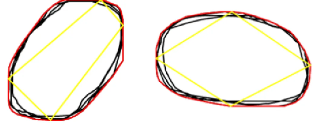
3.1 Difference between P300 and Non-P300 signal. EEG signal in black and the convex hull in red. . . 30

3.2 Special Polygons used in mCALI. . . 31

3.3 Example of Extreme Quadrilateral with the same sketch with different rotations. . . 32

(18)

3.4 Illustration of the intersection feature, using two different sketches but with the same Convex Hull. . . 33 3.5 Bounding box represented in blue and convex hull in red. . . 34 3.6 Representation of the quadrants characteristics. . . 35 3.7 Example of a sketch. In red is the convex hull and in black is the

Alpha-Shape. [Edelsbrunner et al., 1983] . . . 36 3.8 Description of signal with components of creating stimuli. . . 37 3.9 Steps of signal pre-processing. . . 39 3.10 Chart of the results from the Table 3.1, using ALS dataset. Y is the

accu-racy and X the number of intensifications. . . 40 3.11 Chart of the results from the Table 3.2, using ERP-S dataset. Y is the

accuracy and X the number of intensifications. . . 41 3.12 Steps of EEG Signal Pre-Processing. . . 42 3.13 Chart of the results from the Table 3.5, using ALS dataset. Y is the

accuracy and X the number of intensifications. . . 46 3.15 Chart of the results from the Table 3.8, using ALS dataset. Y is the

accuracy and X the number of intensifications. . . 48 3.17 Chart of the results from the best combination that is RBF Gamma 1 and

NPK exponent 15, from Table 3.10 and Table 3.11. Y is the accuracy and X the number of intensifications. . . 50 3.18 Chart of the results from the best combination that is RBF Gamma 1 and

NPK exponent 15, from Table 3.12 and Table 3.13. Y is the accuracy and X the number of intensifications. . . 51 4.1 P300 signal with the regions presented in Table 4.1. . . 57 4.2 Chart of the results using the best classifiers, SVM and Random Forest

with ALS data. Y is the accuracy and X the number of intensifications. . . 58 4.3 Chart of the results using the best classifiers, SVM and Random Forest

with ERP-S data. Y is the accuracy and X the number of intensifications. 59 5.1 Chart of the Table 5.1. Y is the accuracy and X the number of

intensifica-tions. . . 63 5.2 Chart of the Table 5.2, Y is the accuracy and X is the number of

intensifi-cations. . . 64 5.3 Chart of the results from Table 5.3, Y is the accuracy and X is the number

of intensifications. . . 65 xvi

(19)

5.4 Chart of the results of Table 5.4, Y is the accuracy and X is the number of intensifications. . . 66 5.5 Chart of the results of Table 5.5, Y is the accuracy and X is the number of

intensifications. . . 67 5.6 Chart of bars for user dependent test from Table 5.6, Y is the accuracy

and X is the user. . . 68 5.7 Chart of bars for user dependent tests from Table 5.7, Y is the accuracy

and X is the user. . . 69 5.8 Chart of bars for user dependent tests from Table 5.8, Y is the accuracy

and X is the user. . . 70

(20)

(21)

List of Tables

2.1 The advantages and disadvantages from the classifiers. . . 26 3.1 Accuracy results from Non-Normalization and Normalization with ALS

dataset for 5 intensifications to 10 intensifications, using SVM and Ran-dom Forest. . . 40 3.2 Accuracy results from Non-Normalization and Normalization with

ERP-S dataset for 5 intensifications to 10 intensifications, using ERP-SVM and Ran-dom Forest. . . 41 3.3 Results from the feature selection to ALS and ERP-S datasets. . . 43 3.4 Final set of features, resulting from the feature selection process, using

the ALS and ERP-S datasets. . . 44 3.5 Accuracy results for all chosen classifiers with ALS dataset from 5

inten-sifications to 10 inteninten-sifications. . . 45 3.6 Accuracy results from all chosen classifiers with ERP-S dataset from 5

intensifications to 10 intensifications. . . 46 3.7 Vote Systems created, and their composition. . . 47 3.8 Accuracy results from all votes and from SVM using ALS dataset, from

5 intensifications to 10 intensifications. . . 47 3.9 Accuracy results from all votes and from SVM using ERP-S dataset, from

5 intensifications to 10 intensifications. . . 48 3.10 Accuracy results using NPK kernel with ALS dataset from 5

intensifica-tions to 10 intensificaintensifica-tions, for different exponent values. . . 49 3.11 Accuracy results using RBF kernel with SVM using ALS dataset from 5

intensifications to 10 intensifications, for different Gamma values. . . 49 3.12 Accuracy results using NPK kernel with SVM using ERP-S dataset from

5 intensifications to 10 intensifications, for different exponent values. . . . 50 3.13 Accuracy results using RBF kernel with SVM using ERP-S dataset from

5 intensifications to 10 intensifications, for different Gamma values. . . . 50 4.1 All regions of the signal with importance. . . 56 4.2 Accuracy results from two classifiers using ALS dataset from 5

intensifi-cations to 10 intensifiintensifi-cations. . . 58 xix

(22)

4.3 Accuracy results from two classifiers using ERP-S dataset from 5 inten-sifications to 10 inteninten-sifications. . . 58 5.1 Accuracy results for all models using ALS dataset, from 5 intensifications

to 10 intensifications. . . 63 5.2 Accuracy results for all models using ERP-S dataset, from 5

intensifica-tions to 10 intensificaintensifica-tions. . . 63 5.3 Accuracy results when using ALS as training set and ERP-S and GEO to

evaluate, using Geometric and Central Moments models. . . 64 5.4 Accuracy results when using ERP-S as training set and ALS and GEO as

evaluate using Geometric and Central Moments models. . . 65 5.5 Accuracy results when using GEO as training set and ERP-S and ALS to

evaluate, using Geometric and Central Moments models. . . 66 5.6 Accuracy results from user dependent test using ALS dataset. . . 67 5.7 Accuracy results from user dependent test using ERP-S dataset. . . 68 5.8 Accuracy results from user dependent test using GEO dataset. . . 69

(23)

(24)

(25)

Chapter 1 Introduction

In this chapter, we present the motivation, the goals to fulfill, a short description of our solution to detect P300 using geometric properties and Central Moments, as well as our contributions, results and the structure of the document.

1.1 Motivation

Almost everyone can write sentences and words, as well as spell them. However, there are some people who cannot use any motor system for communication. To help these people communicating, Brain Computer Interface (BCI) Applications could be used. BCIs can be used to read brain signals recorded in electroencephalograms (EEG) and allow people to communicate without using movement, just using brain signals.

BCI applications that use P300 Signals to communicate, are mostly Spellers, consist-ing of a matrix of 6-by-6 with letters from the alphabet. These Spellers do not need much training and are easy to use. However, to work they use classifiers to identify the P300 Signals, which need a lot of training and calibrations, becoming a drawback for people who wants to write or communicate fast.

To classify the P300 Signals, there are several approaches using different classifiers. Typically the problem they present as a cost for their high accuracy is the need of indi-vidual training and calibration. So, we intend to create two generic models to detect P300 Signals that can be used at daily tasks quickly and effectively without requiring individual training for each user.

1.2 Goals

The goal of this work is to create two generic P300 signals identifiers. The first one uses the shape of the EEG Signal to detect and classify it as P300 target or P300 non-target using its geometric properties. The second method identifies P300 Signals using Central Moments to describe and classify regions of the signal. These classifiers should not need

(26)

Chapter 1. Introduction 2

individual training or calibration.

We plan to achieve this by finding the best shape features from the P300 signal using its geometric properties for the first classifier, and by peaking the best regions of the EEG Signal that helps us identify the P300 Signal with the second classifier.

Another goal is to compare our two models between them, and also with other ex-isting approaches, to see how they behave in different contexts. In particular, we want to evaluate them in user-independent and user-dependent conditions, as well as using a dataset of signals to create the models and another dataset to test.

1.3 Developed Solution

The solution developed in the context of this work consisted in the creation of two models. One using geometric properties and the other using central moments, to describe and classify P300 Signals.

Existing classifiers used to identify P300, typically require individual training and calibration to achieve good accuracy rates.

The need of training the classifier happens because the EEG Signal varies from user to user, so the classifier needs to adapt to the user that is using the BCI. To overcome this, we created two models that do not need to be individually trained to be used. They already have samples of P300 and Non-P300 signals to help distinguish between the EEG Signals received.

Another problem is the calibration which our models do not need, being ready to be used in almost any circumstance.

1.4 Contribution and Results Obtained

At the end of this dissertation we added two new models to the vast number of classifiers that can detect P300. However, there is a very small sample of classifiers which uses geometric approaches or uses regions of the EEG Signal to identify and classify it.

Our models do not need individual training or calibration which is something that most of current classifiers need. Our models are ready to be used at any time.

With this work we were able to demonstrate that geometric properties or central mo-ments in specified regions of the EEG signal can be used to create a model that detects P300 waves, with a good accuracy.

1.5 Structure of the document

This document is divided in five more chapters. In chapter 2 we present some work related with ours goals, namely the use of shape features of the P300 Signal, and classifiers that

(27)

Chapter 1. Introduction 3

are used to classify P300 signals, as well as a comparison between classifiers. Chapter 3 presents one of the solutions developed, the creation of our Geometric model, describing how to detect P300 and Non-P300 geometrically, the features used and the model settings. Chapter 4 presents the second solution, the creation of a model using Central Moments, defining what central moments are, how to detect P300 based on regions and the settings of the model. Chapter 5 presents the experimental evaluation of our two models and their comparison. Finally, in chapter 6, we present a summary of the dissertation and a conclusion of our work.

(28)

(29)

Chapter 2 Related Work

In this chapter, we present the P300 signal and some approaches, to detect it, enumerating their advantages and disadvantages.

In the second part of the chapter, we describe Spellers based on the P300 paradigm. Finally, we discuss the described works and identify their limitations.

2.1 P300 Signal

In this section, we present the P300 signal, what it is, how to generate it and why and when to use it.

2.1.1 What is?

The firsts recordings of brain activity were done by registering Electroencephalogram (EEG), the first noninvasive method of measuring brain activity for humans. From this method researchers found that electrical potential are specifically time-locked to events, and called it the event related brain potentials (ERP). ERPs are measured brain responses to specific sensory, cognitive or motor events.

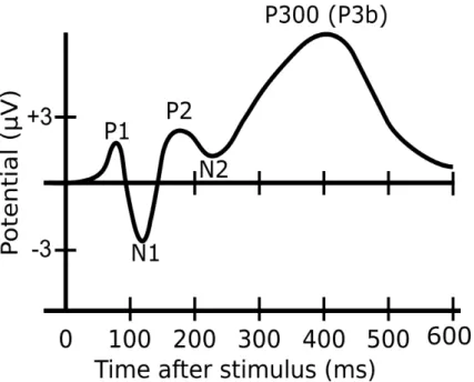
Some components of the ERP use acronyms to indicate what they are. Most of them are referred by the letter N (Negative) or P (Positive), which indicate the polarity of the peak signal, followed by a number indicating the latency in milliseconds or the component ordinal position in the waveform. Some components from the ERP are: P1, N1, P2, N2, P300 (P3a and P3b), P4, N4 and P600.

P300 is one of the peaks of an ERP waveform and one of the most used components. P300 is a positive peak located 300 milliseconds after the stimulus. Figure 2.1 shows the P300 signal and some components of the ERP waveform. The P300 signal can be elicit by either visual, auditory or somatosensory.

At first, the P300 signal was connected to lie detectors because the signal created from the stimulus could not be faked. Thus, the polygraph was used to detect lies. Nowadays

(30)

Chapter 2. Related Work 6

Figure 2.1: Some components from ERP, showing the location of the P300 Signal

it is used in Brain-Computer Interface (BCI) Applications, specially to provide a non-muscular communication channel, particularly for individuals with severe neuronon-muscular disabilities (e.g the Amyotrophic Lateral Sclerosis (ALS)).

The P300 BCI Applications are applications that use this kind of signal, to control the application. P300 Spellers are an example of an application, which uses a matrix with letters to elicit the P300 signal, by alternately lightning its rows and columns.

The P300 has two subcomponents: the novelty of P300 or P3a and the classic P300 or P3b [Polich, 2007]. The P3a is a positive-going amplitude, between 250–280 ms, that displays maximum amplitude over frontal/central electrode sites. The P3a has been as-sociated with brain activity related to the engagement of attention, and the processing of novelty. The P3b is a positive-going amplitude that peaks at around 300 ms and corre-spond to the classical P300. The P3b can be generated with the oddball paradigm, or others paradigms that use the same approach, while the P3a can only be generated with three-stimulus oddball paradigm.

In the context of our work, we will focus on the classical P300.

2.1.2 How to generate?

Around 1988, Farwell and Douchin introduced the P300 BCI, in which they used the oddball paradigm to generate the P300 signal [Farwell and Donchin, 1988]. The oddball paradigm consists in showing a sequence of repetitive stimuli composed by target and non-target, and without noticing the subject’s brain reacts to the target and generates a P300 signal. The P300 target is a stimulus that we want the subject to react and the P300 non-target is a stimulus to which the subject should not react to. Figure 2.2, shows an

(31)

Figure 2.2: Example of an elicited P300 signal, the line in black goes up to potential 3 while not elicited P300 signal does not show that potential

example of a P300 target (black line) and P300 non-target (purple line).

The oddball paradigm is one of the most used approaches to generate P300 signals, presenting both target and non-target stimuli. However, there are other approaches, like the ’single-stimulus’ paradigm [Polich and Heine, 1996] which only present a target stim-ulus, or the three-stimuli oddball paradigm, that is used to elicit the P3a [Wronka et al., 2008], which adds a random non-target stimulus into the mix of the target and non-target stimuli.

EEG signals are collected using several electrodes placed on the scalp according to an international standard electrode montage, called the 10-20 system (Figure 2.3).

(32)

2.1.3 Why and When to use?

P300 is best used in situations that do not require intensive user training because it results from attention-based brain function. It has a wide variety of applications such as those for disabled users in home settings. The applications are relatively fast, effective and easy to use for most users.

P300 signal patterns could change in response to motivation, level of attention, fa-tigue, mental state and learning. Other times, users have unique EEG patterns requiring individualized calibration. To overcome these problems we need advanced digital signal processing algorithms to detect the P300 accurately and quickly.

2.2 Approaches for Detecting P300

In this section we present the main approaches used to detect the P300, focusing on the features and types of classifiers used.

2.2.1 Detection Based on EEG Shape Features

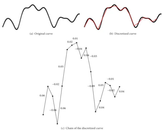
Alvarado-Gonzalez et al., used pattern recognition techniques on EGG signals to detect P300 occurrences [Alvarado-Gonz´alez et al., 2016]. They used a shape-feature vector, containing a contour representation based on an adapted version of the Slope Chain Code (SCC) and the tortuosity measure (a property of the contour) and used a general descriptor (the differences of areas) to describe the differences between curves. Since the SCC is expensive to compute, they adapted the SCC to create the Slope Horizontal Chain Code (SHCC). The SHCC does not compute the angle between two adjacent segments, instead it computes the slope between a segment and the horizontal in the continuous range between -90° and 90°. This way, the segments become independent, and if an electrode is disturbed it will not affect more than one chain element. Also, the SHCC does not require neither rotation invariance, since it is not designed for closed curves, nor scale invariance. To exemplify the process, Figure 2.4 shows a discretized ERP and Figure 2.5 shows the same template curve together with a non-P300 and a P300. The authors also presented an offline calibration algorithm that reduces the dimensionality of the shape-feature vector, the number of trials and the electrodes needed, and described a method to find the template that best represents, for a given electrode, the subject’s P300 based on his own acquired signals.

In the experimental evaluation, authors used EEG signals from 21 students, 8 females and 13 males, between the ages of 21 to 25 years. The ten electrodes used were the Fz, C4, Cz, C3, P4, Pz, P3, PO8, Oz and PO7. They used a P300 word speller, where each row and column from the matrix was intensified 15 times every 125ms in random order, every flash lasted 62.5ms and they extracted 800ms of signal after every stimulus, for

(33)

Figure 2.4: Example of a P300 discretized curve and its resulting chain code by using the SHCC method.

Figure 2.5: Illustration of the difference between a subject’s template curve and (a) a P300 curve and (b) a non-P300 curve.

processing.

To find the best parameters for their algorithm they tested with arbitrarily chosen val-ues, to determine the number of trials to find the template that represented the subject’s

(34)

P300 signal for each electrode. After identifying the parameters, they tested the calibra-tion algorithm using a cross-validacalibra-tion with a training dataset. Results showed that the P300 could be detected with less than fifteen simulations, but eight of the subjects needed no more than five stimulations. The best information was retrieved from electrodes C4, Cz, Fz, Pz, PO7, PO8 and Oz. Electrodes P3, C3 and P4 did not contribute with any relevant information.

After testing the calibration algorithm, they executed two experiments: one test-ing their shape-feature vector with the classifiers Stepwise Linear Discriminant Analysis (SWLDA) and Support Vector Machine (SVM), and another comparing the performance of SWLDA using the shape-feature vector versus the feature vector used by BCI2000 system.

Results from the first experiment revealed that the SWLDA showed best performance than the SVM. The recognition rate for SVM was 87% and for SWLDA was 88%. In the second experiment the percentage of correct classification with the shape-feature vector was 93.15% and with the feature vector used by BCI2000 systems was 83.18%.

In this paper, the authors detect the shape of the signal using templates with similar curves to the P300 signal. This idea requires some individual calibration and training which could be a bit of a downside. The calibration is very important and crucial but if well done assures a good detection of the P300 signal, with a high average accuracy, with less than fifteen stimulations.

2.2.2 Dynamic Time Warping

Concept

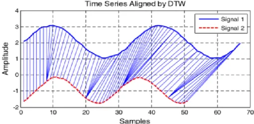
Dynamic time warping is an algorithm for measuring the similarity between two time series. It has been used in the speech domain, to cope with different speaking speeds [Berndt and Clifford, 1994]. In general, it calculates an optimal match between two given temporal sequences with certain restrictions. The DTW does not guarantee the triangle in-equality to hold. Figure 2.6 shows an example of a distance measured with DTW between two signals.

Work by Casarotto

In the work of Casarotto et al [Casarotto et al., 2005], the authors developed a method based on DTW to compute reliable templates of ERP for homogeneous groups of subjects and to automatically quantify the morphological characteristics of the ERPs. As DTW compute a distance between two signals, after aligning them, they used a double-mean technique to pin-point the average value of the distance, to create the template. Figure 2.7 ilustrates the creaton of a template, from two signals, using the technique.

(35)

Figure 2.6: The use of the method with two signals.

Figure 2.7: Creation of the template, using the double-mean technique.

In the experimental evaluation, they had thirty-two children with dyslexia and discrep-ancy. The stimuli were made using a vaccum flourescent display, presenting 21 Italian alphabetic capital and small letters. The persistence of the letters was 25ms. A minimum of four sets of stimuli were presented in the same random order for all the children. The ERPs were recorded during two conditions. The first condition, letter presentation (LPR) was passive, where the subjects passively watched letters without making any effort to read or articulate them silently. The second condition, letter recognition (LRE), was ac-tive: subjects read aloud the letters randomly appearing on the screen after the technician pressed a button.

The electrodes used were Fz, Cz, Pz, Oz, C4, C3, T4, T3, P4 and P3. Authors also captured other information like Electrooculogram (EOG), Electromyograph(EMG), Elec-trocardiogram (ECG) and pneumogram. To improve the signal-to-noise ratio (SNR) of averaged ERPs, a principal component analysis was applied to reduce artifacts from oc-ular movements and blinks. The detection was applied to the 700ms after the stimulus, allowing a reduced time of computation.

(36)

The components extracted were divided by their latency range. The components with latency less than 160ms (P0, N1, P1) belong to the prelexixal period, associated with sen-sory processing of stimuli. The components between 160-420ms (N2, PmaxA, PmaxB, N3) are concerned with stimulus categorization. The components after 420ms (P600a,N4 P600b) reflect long-term semantic memory and feedback processes.

The component P600b is not considered in the results because its latency in individual ERPs is often outside the upper boundary, but the rest of the components were correctly identified 68.56% of the times by the method.

The DTW proved to be useful for improving the comparison between ERPs in dif-ferent subjects, because it reduces the morphological differences between signals. The method proved to successfully measure a significant percentage of the peaks and troughs present on the signal.

Work by Liang and Bougrain

In the work of Liang and Bougrain, authors tested template classifiers that use only one template, such as Point-to-Point averaging (P2P) classifier, Cross-Correlation averaging (CC) classifier and DTW. They also compared those classifiers with other methods that use multiple templates, such as Learning vector quantization (LVQ), multichannel learn-ing vector quantization (mLVQ). To have a better comparison they used also Linear Dis-criminant Analysis (LDA) in the comparison [Liang and Bougrain, 2008].

They used a data set of two subjects, from the BCI competition III, based on the P300 speller. There are 85 letters for training and 100 letters for testing. For each letter, the recording consists of 15 epochs, and with each epoch, there are 12 flashings. For each epoch, a random permutation was chosen to highlight rows and columns. The matrix was 6-by-6 containing twenty-six letters, nine digits and one dash character. The electrodes used are presented in Figure 2.8.

(37)

In the experimental evaluation, the results were based on the raw information from the channel Cz and then by all channels from the two subjects. The results from the Cz channel showed that DTW had an accuracy of 39% and 15% for subject A and B, respectively. However, the classifier LVQ and LDA had better performance. The accuracy for LVQ was 43% and 21%, respectively subject A and B. LDA had an accuracy of 41% and 26% for the same subjects. With all channels, the results were terrible for all one template classifiers, with DTW having an accuracy of 15% and 3% for subject A and B, respectively, resulting in an average of 9% for all 64 channels. Meanwhile, mLVQ and LDA had higher accuracy. MLVQ achieved an accuracy of 87% and 96% for subject A and B, and LDA an accuracy of 88% and 96% for subject A and B.

DTW was not efficient, because producing only one ERP template, has two difficul-ties: first, responses are too noisy to easily distinguish ERP from non-ERP responses and second, it does not take into account the specificities of non-ERP responses to catch small differences between noisy ERP and non-ERP responses.

Work by Chakraborty and Horie

In the work of Chakraborty and Horie, they wanted to reduce the number of electrodes and the time needed to spell a letter, because the BCI spellers, on the market, use 8 electrodes and take 72 seconds to collect data [Chakraborty and Horie, 2016]. They used a cluster that contains signals with similar shape in one group, using DTW, because it would ensure that signals of similar shape, though with certain time delay, will have low distance and would be clustered in the same group. To perform clustering, they used the Ward’s algorithm, a top-down agglomerative algorithm. This algorithm can set a threshold for the inter cluster distances and thus tune the number of clusters visually, using dendrogram.

In the experimental evaluation, they used a speller of 6-by-6 with 26 characters and 10 numerals. All six rows and columns flash for 10 times, randomly. The duration of the flash is 600ms, which means that for a single target character it will take 72 sec. The electrodes used were A1, A2, Fp1, Fp2, Fz, F3, F7, F4, F8, Cz, C3, T3, C4, T4, Pz, P3, T5, P4, T6, O1 and O2.

For the feature selection, they used MultiObjective Genetic Algorithm (MOGA), and for each signal they extracted two features. After that they labelled data from a subject, in signals with and without P300. They used as classifier an artificial neural network, trained using error back propagation.

Results showed that when relevant electrodes are selected for a single individual, it can reduce the number of electrodes to as low as two, and still achieved good recognition with an average accuracy of 67%. They conclude that recognition rate is higher if the subject participated in the experiment several times. Thus, subject training is required to increase concentration during the experiment, and to achieve high recognition rates.

(38)

In conclusion, DTW shows potential as classifier for one electrode only, because it creates one template only, in this way it can create a template for that electrode. However, for multiple electrodes it has some problems. It can be used in other way, like for clas-sifying signals and joining them in cluster, but as classifier of P300 speller it needs more work. The problem the method has is the SNR, since it is hard for it to distinguish ERP from non-ERP response.

2.2.3 Linear Discriminant Analysis

Concept

The Linear Discriminant Analysis (LDA), a generalization from Fisher Linear Discrimi-nant, [Izenman, 2008] [Kantardzic, 2011] is a feature reduction technique which is often used in machine learning and big data with the purpose to find a linear combination of features that can better separate two or more classes. These classes may be identified as species of plants, different types of tumors, etc. To distinguish the known classes from each other, it is used a unique class label. This analysis has two goals: i) discrimina-tion, uses the information to learn and set labels to construct a classifier that will separate predefined classes, ii) classification, that given a set of non-labeled information, use the classifier to predict its class.

Work by Carabalona

Carabalona investigated the differences and performance of the P300 BCI between al-phabetic and icons, and between using the colors white or green as stimulus. The author considered three factors, stimulus type, stimulus color and stimulation timing. In the case of timing it means FAST or SLOW [Carabalona, 2017]. For slow stimulation it flashes 100ms and has a 900ms of dark time between two flashes, for fast stimulation it flashes 60ms and has a dark time of 10ms. It was used data from eight subjects, collected using electrodes Fz, Cz, P3, Pz, PO7, Oz and PO8. It used two spellers, one with alphanumeric characters and another with icons. LDA was used to classify the data, after a phase of training in order to extract and learn how to classify the features.

Results showed that electrodes Pz, PO7 and PO8 had a big impact on the accuracy for the speller with characters. Without those electrodes, the results got worse. The average of accuracy for the speller using stimulus color white and timing fast, was reduced from 94% to 62% when we remove these electrodes. For the same speller using stimulus color green and timing fast the average of accuracy was reduced from 98% to 75%. With timing slow, the speller was not very affected by the removal of these electrodes achieving an average accuracy above 80%.

(39)

Work by Selim et al

Selim et al, wanted to test the performance of different machine learning algorithms for the P300 Speller paradigm based on accuracy [Selim et al., 2009]. The algorithms chosen were Bayesian Linear Discriminant Analysis (BLDA), Linear Support Vector Machine (SVM), Fisher Linear Discriminant Analysis (FLDA), Generalized Anderson’s Task lin-ear classifier (GAT) and LDA.

They used a data set of two subjects collected using all 64-channels, from the BCI competition III, based on the P300 speller. There are 85 letters for training and 100 letters for testing. For each letter, the recording consists of 15 epochs, and with each epoch, there are 12 flashings. For each epoch, a random permutation was chosen to highlight rows and columns. The matrix was 6-by-6 containing twenty-six letters, nine digits and one dash character.

Results showed that BLDA and SVM had better performance. The accuracy with 15 epochs for BLDA was 98% and SVM was 97%. Meanwhile, LDA had an accuracy of 83%.

LDA being one of the oldest classifiers is still considered one of the best for classi-fication, because of its simplicity, being fast to classify and giving robust classification. However, it has some problems, specially if we increase the input feature spaces, it could begin to deteriorate with insufficient number of training samples. The need for training is essential for this classifier to predict the P300 signal.

2.2.4 Stepwise Linear Discriminant Analysis

Concept

Stepwise Linear Discriminant Analysis (SWLDA) is a technique used to select predic-tor variables that are include in a multiple regression model [Krusienski et al., 2008] [Draper and Smith, 1981]. It does a combination of forward and backward stepwise re-gression adding the most statistically significant predictor variable. After each new entry to the model, it does a backward stepwise regression to remove the least significant vari-ables. This process is done until the model includes a predetermined number of terms or until no additional terms satisfy the entry criteria. SWLDA is one of the most efficient classifiers because the result happens with a non-exhaustive way. This provides an auto-matic feature extraction because unimportant terms are removed from the model, and thus we will have less training data to corrupt the classification result.

Work by Krusienski et al

Krusienski el al, performed a study to discover if using a larger set of electrodes, the per-formance of SWLDA would increase [Krusienski et al., 2008]. They used seven subjects, with the task to focus attention on a specified letter of the matrix. The rows and columns

(40)

were intensified for 100ms with 75ms between intensifications. They analyzed 800ms segments of data after the stimulus. They used a collection of channels sets illustrated in Figure 2.9.

Figure 2.9: The 64-channel electrode montage and the channel sets. Set 0 is a subset defined purely for illustration purposes, sets 1–4 were used in the analysis.

Before the experimental evaluation, the classifier was calibrated to find the best fea-tures followed by four factors: channel set, reference, decimation factor and maximum features.

The results showed that the accuracy from using a larger set of electrodes to detect P300 is higher than using a small set of electrodes. The average accuracy for the larger set containing the electrodes from the Set 4 showed in Figure 2.9 was higher than 80%. Meanwhile, using the electrodes from the Set 1, the average accuracy was between 50-60%.

Work by Speier et al

Speier el al, compared an hidden Markov model (HMM), SWLDA and a naive Bayes clas-sifier (NB) with the intend of finding which one was better [Speier et al., 2014]. HMM treats typing as a sequential process where each character selection is influenced by pre-vious selections. The authors performed two studies, one offline and another online. For the offline study, they used ten subjects. For the online study, they used five subjects. The speller used a system of 6-by-6 matrix with a inter-stimulus interval (ISI) of 125ms. The

(41)

electrodes used were all 64-channels. The evaluation performed was based on selection rate, accuracy and information transfer rate.

Results for the offline study showed that the accuracy of the SWLDA was better than the other two classifiers with an accuracy of 88.82%. Meanwhile, NB and HMM were not far, with 88.81% and 88.34% accuracy, respectively.

The results for the online study were different with HMM having the best accuracy, with 92.34%. However, SWLDA had an accuracy of 91.68% and NB an accuracy of 82.83%.

2.2.5 Support Vector Machine

Concept

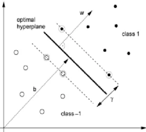
The Support Vector Machine (SVM) [Kaper et al., 2004] which is another way to do bi-nary classification by creating a hyperplane described by the weight vector w and the bias term b as illustraded in Figure 2.10. This algorithm needs to acquire a hyperplane that suites a optimally criterion, by doing a projection on the weight vector. This projection would show the predicted class label. Instead of having several possible choices, it is best if it is chosen the maximum margin criterion, because it favors the hyperplane with the largest separation margin. The optimal hyperplane is best described by support vectors because those are the only vectors necessary.

Figure 2.10: SVMs find the optimal hyperplane (solid line) to separate two classes by maximizing the margin . It can be described by the vector γ and the bias term b. Only support vectors (bordered circles) are necessary to calculate w and b.

(42)

Work by Kaper et al

Kaper et al, used SVM for classifying EEG signals to detect absence or presence of the P300 [Kaper et al., 2004]. They used a P300 speller paradigm represented in a 6-by-6 matrix, containing 36 symbols. Each row and column was intensified once within one trial, if the desired symbol gets intensified it is elicited a P300. The algorithm was trained with a training set labeled with ”1” and ”-1” for P300 presence/absence.

They took 600ms after stimulus from electrodes Fz, Cz, Pz, Oz, C3, C4, P3, P4, PO7 and PO8. For each trial, twelve epochs for the different rows and columns exist, in which two should contain P300 and the other ten should not.

Results using a five-fold cross-validation on the training set showed an accuracy of 84.5% for separation of P300 from non-P300 epochs. It also showed that error rates decrease with the number of repetitions from 35.5% to 0.0%, and the correct solution was found after only five repetitions.

When using the P300 speller paradigm with SVM in a very fast EEG-Based BCI, they achieved rates up to 84.7 b/min. Because the use of several electrodes could ruin the procedure, authors used only ten electrodes from the 64 electrodes. One advantage of this approach is the low preprocessing required, which is appropriate for an online solution.

Work by Mirghasemi et al

In the study of Mirghasemi et al, authors compared five classifiers to test their perfor-mance. The classifiers chosen were SVM, Gaussian Support Vector Machine (RSVM), Neural Network (NN), Fisher Linear Discriminant Analysis (FLDA) and Kernel Fisher Discriminant (KFD) [Mirghasemi et al., 2006].

In the experimental evaluation, they used the dataset from BCI 2003 competition that used P300 Speller with a matrix of 6-by-6, containing 36 symbols. All rows and columns were randomly intensified and the intensifications of each row and column were repeated for 15 times. The dataset recorded all 64 electrodes, but authors only used Fz, Cz, Pz, Oz, P3, P4, C3, C4, PO7 and PO8 electrodes.

They used Principal Component Analysis (PCA) to perform feature reduction, de-creasing from 144 features to 21, and thus reducing the classification time.

Results showed perfect performance with 100% accuracy after 4 trials for several methods, namely FLDA, FKD, SVM and RSVM.

Work by Thulasidas et al

Thulasidas et al, implemented a P300 Speller using SVM as classifier and a novel feature [Thulasidas et al., 2006]. The author also performed various studies on the data to mini-mize the training time required, by conducting a study to minimini-mize the number of rounds

(43)

needed for training, using an SVM model created with a subset of the training data. The results were that with two rounds for each character, the accuracy was 82.7%.

In the experimental evaluation, they used a P300 Speller with a 6-by-6 matrix of char-acters. All rows and columns were randomly intensified for 100ms, followed by 75 ms of no intensification. They collected data from nine subjects using 25 electrodes. The manual electrodes selected were C3, C4, Cz, CPz, and FCz, plus two distant positions P7 and P8.

Results showed an average accuracy of 95%, taking 22 seconds for each character. The time needed for training is normally 20 minutes. However, with their method of minimizing the time required for training, the training was reduced to ten minutes.

The SVM can be used as a linear classifier and as a non-linear classifier. Although it has a low processing time as classifier, it requires some time for training. In the case of a non-linear approach, we have also the problem of over-fitting, because it can model a training data very accurately but it can fail if the training data are not all representative of independent test data. SVM as another drawback that is the process of attaining suitable model and training parameters.

2.2.6 Peak Picking and Area

The Peak Picking analysis [Farwell and Donchin, 1988] is obtained by doing the differ-ence between the lowest negative point previously from the P300 window and the highest positive point in the P300 window, as illustrated in Figure 2.11.

Figure 2.11: Graphical representation of the temporal evolution of a P300 EEG signal, highlighting in red the peaks used in the Peak Picking method.

Peak picking is not sensitive to latency variability, because the P300 peak can be lo-cated anywhere in a relatively wide time window. However, at a short inter-stimulus

(44)

interval (ISI) it becomes a weakness. Since, the peak picking algorithm looks for a maxi-mum value at any point, it is susceptible to falsely attributing a P300 peak generated by a previous stimulus.

The area analysis [Farwell and Donchin, 1988], takes all the points in a broad range, in other words calculates the ’area under the curve’ [Sansana, 2016] between 250ms and 600ms of a P300 from an EEG signal as presented in Figure 2.12. This way it became purely additive instead of multiplicative, and it does not require a training set. This algo-rithm misses some information contained in a consistent distinctive ERP shape and time course and avoids some noise. Hence, it has the advantage of information contained in a broad flat ERP.

Figure 2.12: Graphical representation of the temporal evolution of a P300 EEG signal, highlighting in light blue the zone defined for the Area analysis.

In this study [Farwell and Donchin, 1988], the authors used three females and one male subjects. They used their 6-by-6 matrix containing letters of the alphabet, as well as several 1-word commands for controlling the system. Each row and columns was intensified for a period of 100msec. For the first session the ISI was 500msec, in the second session they acquired the data with both a 500msec and a 125msec ISI. The task was for the subjects to attend to a given letter and to keep a running mental count of the number of times it flashed.

The data used of the EEG was 600msec after the onset of each flash. They used four different algorithms to compute the time needed to reach an acceptable accuracy: SWLDA , Peak Picking, Area and Covariance classifiers.

Results showed that SWLDA and peak picking proved to be the most efficient algo-rithms. At 125 msec ISI, SWLDA was the fastest to reach 80% and 95% accuracy with average of 23 seconds and 41 seconds, respectively. At 500 msec, peak picking was the fastest to reach 80% and 95% accuracy with an average of 21 seconds and 33 seconds,

(45)

respectively. The area, took longer (50 seconds) to reach 80% and 95% accuracy.

2.3 P300 Spellers

The first speller was presented in [Farwell and Donchin, 1988], and it was a matrix of 6-by-6 containing the letters of the alphabet plus 1-word commands, as illustrated in Figure 2.13. The speller works by intensifying each of the 6 rows and columns for a period of time with an inter-stimulus interval (ISI) between intensifications. It flashes the column or row and the subject should focused on the cell (column and row) that is intensified to elicit the P300. This speller achieved a mean character selection accuracy of 85-90%.

One of the great advantages of the P300 BCI is that it does not require intensive user training, since P300 components result from endogenous attention-based brain function.

There are some issues with P300-based BCI, like the fact that the EEG signal patterns change in response to factors like motivation, level of attention, fatigue, mental state, learning, and other nonstationarities that exist in the brain. Other problems are that users may have unique EEG patterns that make it necessary for individualized calibration.

Figure 2.13: First interface of P300 Speller

One area of research has been to modify the type of visual stimulus or other stimulus to potentially elicit stronger P300, using superior flashing methods by using character mo-tion, changing the size and sharpness from the character, attributing stimulus colors, vary-ing the grid layout, increasvary-ing stimulus contrast or stimulus presentvary-ing ”famous faces” [Speier et al., 2017], or using varied geometric pattern stimulus [Ma and Qiu, 2017] and using icon-spellers [Carabalona, 2017].

Here we present some new paradigms for communication like the Single Character (SC) speller [Fazel-Rezai et al., 2012] that consists in randomly flashing one character at a time with a brief delay between flashes. The SC speller has a longer delay between flashes than the row/column speller (RC), allowing character classification with fewer flashes per character. The row/column flasher is about two times faster than the SC flasher. However,

(46)

the SC speller results in larger P300 amplitudes compared to the RC speller. The accuracy results for this speller reached 77.9%.

The Checkerboard Speller (CB) [Fazel-Rezai et al., 2012] [Townsend et al., 2010], was designed to correct two problems. The first is the elimination of instances when the same character flashes twice in succession. The second, is the reduction of the amount of dis-traction and/or inherent noise. Experimental evaluation of CB Speller, showed that it produced significant improvements in accuracy. The overall spelling accuracy for this speller was 90.6%. The CB disassociates the rows and columns of the matrix, eliminating double flashes and significantly reducing distraction, by using a matrix of 8 x 9, composed with 72 items as represented in Figure 2.14. The items in the white squares randomly pop-ulate one 6 x 6 matrix and the items in the black squares randomly poppop-ulate a second 6 x 6 matrix. It is prohibited simultaneous adjacent flashes by the segregation of adjacent items into separate flash groups. The characters flashes are in sequential order: first, the rows of the white matrix, second, the rows of the black matrix, third, the columns of the white matrix and fourth, the columns of the black matrix are flashed. After all rows and columns in both matrix have been flashed, the characters in the matrix are re-randomized and the next sequence of flashes begins.

Figure 2.14: Example of the CheckerBoard Speller.

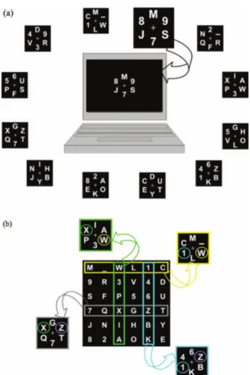
The Region based paradigm, that works by flashing several regions instead of rows or columns [Fazel-Rezai et al., 2012]. It decreases the near-target effect and human error and adjacency problem. Overall, the speller does character recognition in two levels. The first level, the characters are placed in seven groups located in different regions of the screen. Similar to the P300 BCI paradigm, to select the desired group the user attend to a specific character in one of the seven groups while each group randomly flashes. The second level, individual characters of the selected group are distributed into the seven regions. Similarly to the first level, different regions are flashed while the subject attends to one region, to select the desired character. The spelling accuracy from the results were 86.1%. Figure 2.15 is an example of the speller, at left shows the first level, on the right

(47)

shows the second level.

Figure 2.15: Example of the Region-based paradigm.

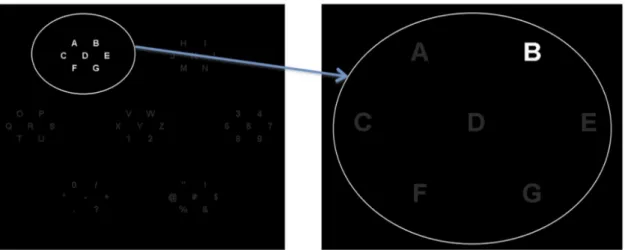
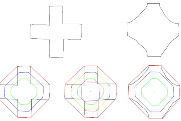
Aloise et al, focused a study in selective attention, where the subject can focus his at-tention on a specific target of the visual field overt and covert atat-tention [Aloise et al., 2012]. Overt attention relates to the condition in which the subject turns his gaze toward the tar-get. Covert attention, the subject focuses his attention on the target without gazing at it directly. The authors were influenced by the covert attention to develop the GeoSpell. The characters are organized with the same logic as the first speller as N by N matrix. Characters are grouped into 2N sets of N characters. With that kind of presentation, each character belongs to exactly two sets. In each set the characters are displayed at the vertices of a regular geometric figure. During the presentation, the set of characters are display sequentially on the screen and the characters are displayed at the same position for each of the two sets. All 2N sets are shown in a pseudo-random sequence that is repeated several times in a trial. A fixation point is shown in the centre to help the subject avoid eye movements.

In the experimental evaluation, the authors compared the P300 Speller and GeoSpell. The electrodes used were Fz, Cz, Pz, Oz, P3, P4, PO7 and PO8 for both Spellers. Results showed that P300 Speller had a better accuracy, with 96.17%. Meanwhile, the GeoSpell had an accuracy of 77.82%.

From the Spellers presented, the only one that showed promising results was the Checkerboard paradigm, because it was the only one that had a higher accuracy than the normal. Meanwhile, the others Spellers showed new ways to elicit the P300, but they did not reached the desired performance that would surpass its precedent.

2.4 Discussion

In this section we discuss about the performance of the classifiers described previously, to find the better classifier of P300 Signal. We also analyze the existing spellers presenting

(48)

Figure 2.16: (a) Example of GeoSpell. (b) Group organization. Each group contains the characters of one row or one column of matrix.

their advantages and disadvantages.

The work of Alvarado-Gonzalez et al, is related to our goal to detect the P300 sig-nal because it uses the shape of the sigsig-nal to detect other sigsig-nals with the same shape [Alvarado-Gonz´alez et al., 2016]. In this case, they created templates with similar curves of the P300 signal. However, for our solution the detection of P300 signal needs to be fast and should not require calibration, which is the problem they face. In their method the calibration is very important and crucial. If well done it results in a good detection of the P300 signal, with an accuracy of 88% using the classifier SWLDA.

Another algorithm that is related to our work is Dynamic Time Warping, because it can be used to create templates from P300 signals by measuring the similarity between two time series. However, it is not a very reliable classifier. When used with a single electrode the accuracy can be around 50%, while with the collection of 64 electrodes, the classifier had an average accuracy of 9%. The major problem from the method is the SNR, since it is hard for it to distinguish ERP from non-ERP response.

(49)

A classifier to be useful need to be fast during classification, require little or no train-ing, and have a good accuracy. We presented some classifiers that are used nowadays, like the LDA, the SWLDA and SVM, and others that are not that much mention in the community like the Area and the Peak Picking.

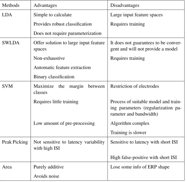
We present in Table 2.1 the advantages and disadvantages of them. The algorithms Peak Picking and Area are not fast enough in detecting P300, they take a lot of time. The Peak Picking is good only when there is a high ISI time, and it can detect P300 much more faster than the SWLDA.

One problem found is that all of the classifiers need individual training.

SVM has a low processing time as classifier, but requires time to be trained. From the study of Thulasidas et al, it needs about 10 minutes to train and is a very complex algorithm to parameterize [Thulasidas et al., 2006]. However, the average accuracy is very high.

The LDA, being one of the oldest classifier, is still one of the best, because of its simplicity and speed to classify. However, it has problems when the input feature space increases it could begin to deteriorate with insufficient number of training set.

The SWLDA is one of the most efficient classifiers because the result happen with a non-exhaustive way and offers a solution to the problem the LDA has that is the large input feature spaces. However, it requires time for training and calibration that is crucial to the classifier.

One aspect that is important for detecting P300 is the identification of the best set of electrodes. The most used electrodes by our studies are Fz, C4, Cz, C3, P4, Pz, P3, PO8, Oz and PO7. The less used are O1, O2, FCz, CPz, P7, P8, T4 and T3. From studies between 2015-2017, the most used electrodes were Fz, Cz, Pz, P3, P4, Oz, O1, O2, C3 and C4 [Turnip et al., 2017] [Combaz and Van Hulle, 2015] [Vareka and Mautner, 2015] [Zhang et al., 2016] [Zeyl et al., 2016] [Yin et al., 2015] [Cecotti, 2015] [Akram et al., 2015]. Some also used PO7, PO8, P7 and P8 electrodes.

In the case of the spellers, there exists a lot of adaptations from the first speller, using character motion, changing the size and sharpness of the characters, using stimulus colors, varying the grid layout, increasing stimuli contrast or stimuli presenting ”famous faces”, or using varied geometric pattern stimuli and using icons-spellers.

The spellers studied that showed best accuracy with different layout than the normal speller was the Checkerboard Speller with an accuracy of 90.6%, while with the normal speller the accuracy was between 85% and 90%. One of Checkerboards’s problems is that it could be very complex to develop because it uses a matrix of 8-by-9 with 72 items divide by two colors. Region-based paradigm, Single Character speller and GeoSpell are not very promising because the accuracy was smaller than the P300 Speller. For simplicity the best choice is the normal P300 speller, because it is more easy to generate and it is used a lot by the community.