WO R K I N G PA P E R S E R I E S

(1)

WO R K I N G PA P E R S E R I E S

N O 7 1 1 / J A N UA RY 2 0 0 7

WHAT “HIDES”

BEHIND SOVEREIGN

DEBT RATINGS?

(2)

In 2007 all ECB publications feature a motif taken from the

€_{20 banknote.}

WO R K I N G PA P E R S E R I E S

N O 7 1 1 / J A N U A RY 2 0 0 7

This paper can be downloaded without charge from http://www.ecb.int or from the Social Science Research Network electronic library at http://ssrn.com/abstract_id=954705.

WHAT “HIDES” BEHIND

SOVEREIGN DEBT RATINGS?

1

by António Afonso

2

_{, Pedro Gomes}

3

and Philipp Rother

4

(3)

© European Central Bank, 2007

Address Kaiserstrasse 29

60311 Frankfurt am Main, Germany

Postal address Postfach 16 03 19

60066 Frankfurt am Main, Germany

Telephone +49 69 1344 0

Internet http://www.ecb.int

Fax

+49 69 1344 6000

Telex 411 144 ecb d

Any reproduction, publication and reprint in the form of a different publication, whether printed or produced electronically, in whole or in part, is permitted only with the explicit written authorisation of the ECB or the author(s).

The views expressed in this paper do not necessarily reflect those of the European Central Bank.

(4)

In this paper we study the determinants of sovereign debt credit ratings using rating notations from the three main international rating agencies, for the period 1995-2005. We employ panel estimation and random effects ordered probit approaches to assess the explanatory power of several macroeconomic and public governance variables. Our results point to a good performance of the estimated models, across agencies and across the time dimension, as well as a good overall prediction power. Relevant explanatory variables for a country's credit rating are: GDP per capita, GDP growth, government debt, government effectiveness indicators, external debt, external reserves, and default history.

JEL: C23; C25; E44; F30; F34; G15; H63

(6)

Non-technical summary

Sovereign credit ratings are a condensed assessment of a government’s ability and

willingness to repay its public debt both in principal and in interests on time. In this,

they are forward-looking qualitative measures of the probability of default put forward

by rating agencies. This paper studies the determinants of sovereign debt credit ratings

of the three main international rating agencies: Standard and Poor’s, Moody’s and Fitch

Ratings. We build an extensive ratings database, with sovereign foreign currency

ratings, attributed by the three agencies, as well as the credit rating outlook, for a panel

of 130 countries from 1970 to 2005.

In the first part of the paper we explain the main econometric approaches to the study of

the determinants of credit ratings focussing on specification of the functional form and

the estimation methodology. There are two major strands of empirical work in the

literature: on the one hand, OLS analysis on a numerical representation of the ratings,

which allows for a straightforward generalization to panel data by doing fixed or

random effects estimation; on the other hand, ordered response models. We discuss in

some detail the main advantages and caveat of the several approaches and suggest an

original specification and a more robust estimation procedure. Our specification allows

for an important distinction between short and long-run impact of the explanatory

variables on the credit rating.

In terms of the regressors, we divide them in four main blocks: macroeconomic

performance (per capita GDP, unemployment rate, inflation rate, real GDP growth),

government performance block (government debt, fiscal balance and government

effectiveness), external balance (external debt, foreign reserves and current account

balance) and other explanatory variables (default history, European Union and regional

dummies).

The main finding is that GDP per capita, real GDP growth, government debt,

government effectiveness, external debt and external reserves, sovereign default

indicator as well as being a member of European Union, are the most important

determinants of the sovereign debt ratings. We find that the government related

(7)

The large sample allows for a sub-period analysis and for a differentiated analysis of

high and low ratings. While the results are roughly stable across agencies, time periods

and ratings levels, some additional interesting results emerge. For instance, for the low

rating levels, external debt and external reserves are more relevant. On the other hand,

for the early sub-period, 1996-2000, the current account balance was more important,

while external reserves were possibly somewhat more important in the later period,

2001-2005 (for Moody’s and S&P). Moreover, after the Asian crisis, it seems there was

a decline in the relevance of the current account variable in the specifications for

Moody’s and S&P.

In the last part of the paper we analyse some specific country cases. We find that, for

instance, Spain’s rating upgrades since 1998 were mainly due to its good

macroeconomic performance, while Portugal’s deterioration of its creditworthiness

during the same period can be mainly attributed to poor government performance.

Additionally new European Union member countries benefited not only from their good

macroeconomic performance, but also from a credibility effect of joining the European

(8)

1. Introduction

Sovereign credit ratings are a condensed assessment of a government’s ability and

willingness to repay its public debt both in principal and in interests on time. In this,

they are forward-looking qualitative measures of the probability of default put forward

by rating agencies. Naturally, one should try to understand the determinants of credit

ratings, given their relevance for international financial markets, economic agents and

governments. Indeed, sovereign credit ratings are important in three ways. First,

sovereign ratings are a key determinant of the interest rates a country faces in the

international financial market and therefore of its borrowing costs. Second, the

sovereign rating may have a constraining impact on the ratings assigned to domestic

banks or companies. Third, some institutional investors have lower bounds for the risk

they can assume in their investments and they will choose their bond portfolio

composition taking into account the credit risk perceived via the rating notations. For

instance, the European Central Bank when conducting open market operations can only

take as collateral bonds that have at least a single A attributed by at least one of the

major rating agencies.

In this paper we perform an empirical analysis of foreign currency sovereign debt

ratings, using rating data from the three main international rating agencies: Fitch

Ratings, Moody’s, and Standard & Poor’s. We have compiled a comprehensive data set

on sovereign debt ratings, macroeconomic data, and qualitative variables for a wide

range of countries starting in 1990. Regarding the empirical modelling strategy, we

follow the two main strands in the literature. We make use of linear regression methods

on a linear transformation of the ratings and we also estimate our specifications under

an ordered probit response framework.

Our main contribution to the existing literature is the innovation of the estimation

method used and the functional form specification, and the large dataset employed.

Under the linear framework, we argue that random effects estimation will be inadequate

due to the correlation between the country specific error and the regressors, but also that

its alternative, fixed effects estimation will not be very informative. We salvage the

random effects approach by means of modelling the country specific error, which in

(9)

time-invariant regressors. This setting will allow us to make the constructive distinction

between immediate and long-run effects of a variable on the sovereign rating.

Moreover, we also use a limited dependent variable framework by estimating the

augmented-model using ordered probit and random effects ordered probit specifications.

The latter is the best procedure for panel data as it considers the existence of an

additional normally distributed cross-section error. This approach allows both to

determine the cut-off points throughout the rating scale as well as to test whether a

linear quantitative transformation of the ratings is actually more appropriate than a

possible non-linear transformation. Furthermore, we perform robustness check by

allowing for a sub-period analysis and for a differentiated high and low rating analysis.

We find that in particular six core variables have a consistent impact on sovereign

ratings. These are the level of GDP per capita, real GDP growth, the public debt level

and government effectiveness, as well as the level of external debt and external

reserves. A dummy reflecting past sovereign defaults is also found significant as well

as, in some cases, the fiscal balance and a dummy for European Union countries. It is

noteworthy that fiscal variables turn out to be more important than found in the previous

literature.

The paper is organised as follows. In Section Two we give an overview of the rating

systems and review the relevant related literature. Section Three explains our

methodological choices, specifically regarding the econometric approaches employed.

In Section Four we describe the dataset and report on the empirical analysis, notably in

terms of the estimation and prediction results. Section Five summarises the paper’s

main findings.

2. Rating systems and literature

2.1. Overview of rating systems

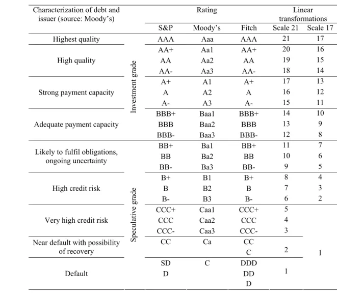
We use sovereign credit ratings by the three main international rating agencies,

Moody’s, Standard & Poor’s (S&P) and Fitch Ratings. Although these agencies do not

use the same qualitative codes, in general, there is a correspondence between each

(10)

rating in descending order form AAA to CCC-, while Moody’s system goes from Aaa

to Caa3.

[Insert Table 1 here]

2.2. Literature review

Sovereign ratings are assessments of the relative likelihood of default. The rating

agencies assess the risk of default by analysing a wide range of elements from solvency

factors that affect the capacity to repay the debt, but also socio-political factors that

might affect the willingness to pay of the borrower. For example, S&P determines the

rating by evaluating the country’s performance in each of the following areas: political

risk, income and economic structure, economic growth and prospects, fiscal flexibility,

general government debt burden, off-shore and contingent liabilities, monetary

flexibility, external liquidity, public-sector external debt burden and private sector

external debt burden.

Given that the rating materializes out of the analysis of a vast amount of data, it would

be useful to find a reduced set of variables capable of explaining a country’s rating. A

first study on the determinants of sovereign ratings by Cantor and Packer (1996)

concluded that the ratings can be largely explained by a small set of variables namely:

per capita income, GDP growth, inflation, external debt, level of economic

development, and default history. Further studies incorporated more variables.

Macroeconomic performance variables like the unemployment rate or the

investment-to-GDP ratio. In papers focussing on the study of currency crises several external

indicators such as foreign reserves, current account balance, exports or terms of trade

seem to play an important role. Moreover, indicators of how the government conducts

its fiscal policy, budget balance and government debt can also be relevant, as well as

variables that assess political risk, like corruption or social indexes. Table 2 summarises

some of the relevant related studies and findings.

(11)

Regarding the econometric approach, there are two major strands in the literature. The

first uses linear regression methods on a numerical representation of the ratings. The

early study by Cantor and Packer (1996), applies OLS regressions to a linear

representation of the ratings, on a cross section of 45 countries. This methodology was

also pursued by Afonso (2003), Alexe et al. (2003) and Butler and Fauver (2006). Using

OLS analysis on a numerical representation of the ratings is quite simple and allows for

a straightforward generalization to panel data by doing fixed or random effects

estimation (Monfort and Mulder, 2000; Eliasson, 2002 and Canuto et al., 2004).

Although estimating the determinants of ratings using these approaches has in general a

good fit and a good predictive power it faces some critiques. As ratings are a qualitative

ordinal measure, using traditional estimation techniques on a linear representation of the

ratings is not the most adequate framework of estimation. First, it implies the

assumption that the difference between two rating categories is equal for any two

adjacent categories, which would need to be tested. Furthermore, even if this

assumption was true, because of the presence of elements in the top and bottom

category, the estimates are biased, even in big samples. Nevertheless, Eliasson (2002)

argues that given the existence of many categories one can treat the rating variable as

continuous and to overcome the criticism of the assumption of an even distance between

steps, it is possible to use different quantitative transformations. For instance, Reisen

and Maltzan (1999) apply a logistic transformation of the ratings and Afonso (2003)

applies both a logistic and an exponential transformation of the ratings. In that case, the

differences between categories are not constant, but are still imposed a priori.

The other strand of the literature uses ordered response models. Because the ratings are

a qualitative ordinal measure, the established wisdom advises the use of ordered probit

estimation. This method will itself determine the size of the differences between each

category. For example, this procedure was used by Hu et al. (2002),

Bissoondoyal-Bheenick (2005) and Bissoondoyal-Bissoondoyal-Bheenick et al. (2005). Although this should be

considered the preferred estimation procedure it is not entirely satisfying. The crucial

point is that the ordered probit asymptotic properties do not generalise for a small

sample, so if we estimate the determinants of the ratings using a cross-section of

countries, we would have too few observations. It is therefore imperative to try to

(12)

be careful. Indeed, the generalization of ordered probit to panel data is not completely

straightforward, due to the existence of a country specific effect. Furthermore, within

this framework, the need to have many observations makes it harder to perform

robustness analysis by, for instance, partitioning the sample. In Section Three we will

address these questions when explaining our modelling strategy.

3. Methodology

Using a linear scale we grouped the ratings in 17 categories, by putting together in the

same bucket the few observations below B-. Indeed, if we used a specific number for

each existing rating notch, for instance 21 categories, it might be hard to efficiently

estimate the threshold points between CCC+ and CCC, CCC and CCC- and so on, given

that the bottom rating categories have very few observations. Table 1 above also shows

the relation established between the qualitative and the possible linear scales. Moreover,

and as we will see latter in the paper, a linear transformation is quite adherent to the

data. Nevertheless, we also report in Appendix 3 estimation results using a logistic

transformation.

3.1. Explanatory variables

Building on the evidence provided by the existing literature, we identify a set of main

macroeconomic and qualitative variables that may determine sovereign ratings.

GDP per capita – positive impact on rating: more developed economies are expected to

have more stable institutions to prevent government over-borrowing and to be less

vulnerable to exogenous shocks.

Real GDP growth – positive impact: higher real growth strengthens the government’s

ability to repay outstanding obligations.

Inflation – uncertain impact: on the one hand, it reduces the real stock of outstanding

government debt in domestic currency, leaving overall more resources for the coverage

of foreign debt obligations. On the other hand, it is symptomatic of problems at the

(13)

Unemployment – negative impact: a country with lower unemployment tends to have

more flexible labour markets making it less vulnerable to changes in the economic

environment. In addition, lower unemployment reduces the fiscal burden of

unemployment and social benefits while broadening the base for labour taxation.

Government debt – negative impact: a higher stock of outstanding government debt

implies a higher interest burden and should correspond to a higher risk of default.

Fiscal balance – positive impact: large fiscal deficits absorb domestic savings and also

suggest macroeconomic disequilibria, negatively affecting the rating level. Persistent

deficits may signal problems with the institutional environment for policy makers.

Government effectiveness – positive impact: high quality of public service delivery and

competence of bureaucracy should impinge positively of the ability to service debt

obligations. (We initially used all six World Bank Governance Indicators: voice and

accountability, political stability, regulatory quality, rule of law, control of corruption

and government effectiveness, but only this last one turned up as significant).

External debt – negative impact: the higher the overall economy’s external

indebtedness, the higher becomes the risk for additional fiscal burdens, either directly

due to a sell-off of foreign government debt or indirectly due to the need to support

over-indebted domestic borrowers.

Foreign reserves – positive impact: higher (official) foreign reserves should shield the

government from having to default on its foreign currency obligations.

Current account balance – uncertain impact: a higher current account deficit could

signal an economy’s tendency to over-consume, undermining long-term sustainability.

Alternatively, it could reflect rapid accumulation of fixed investment, which should lead

to higher growth and improved sustainability over the medium term.

Default history – negative impact: past sovereign defaults may indicate a great

(14)

by a dummy variable indicating the past occurrence of a default and by a variable

measuring the number of years since the last default. This variable measures the

recovery of credibility after a default and can be expected to influence positively the

rating score.

3.2. Linear regression framework

A possible starting point for our linear panel model would follow Monfort and Mulder

(2000), Eliasson (2002) or Canuto, Santos and Porto (2004), generalizing a cross section

specification to panel data,

it it i i it

R =βX +λZ +a +µ , (1)

where we have: R – quantitative variable, obtained by a linear or by a non-linear

transformation; Xit is a vector containing time varying variables that includes the

time-varying explanatory variables described above and Zi is a vector of time invariant

variables that include regional dummies.

In (1) the index i (i=1,…,N) denotes the country, the index t (t=1,…,T) indicates the

period and ai stands for the individual effects for each country i (that can either be

modelled as a error term or as N dummies to be estimated). Additionally, it is assumed

that the disturbances µit are independent across countries and across time.

There are three ways to estimate this equation: pooled OLS, fixed effects or random

effects estimation. In normal conditions all estimators are consistent and the ranking of

the three methods in terms of efficiency is clear: a random effects approach is preferable

to the fixed effects, which is preferable to pooled OLS. The question one should ask is

whether the normal conditions are fulfilled. What we mean by normal conditions is

whether or not the country specific error is uncorrelated with the regressors E(ai| Xit,

Zi)=0. If this is the case one should opt for the random effects estimation, while if this

condition does not hold, both the pooled OLS and the random effects estimation give

(15)

In our case, it seems more natural that the country specific effect is correlated with the

regressors.1 Given this scenario one should be tempted to say that the “fixed effects

estimation” is the best strategy, but that has a problem. Because there is not much

variation of a countries rating over time, the country dummies included in the regression

will capture the country’s average rating, while all the other variables will only capture

movements in the ratings across time. This means that, although statistically correct, a

regression by fixed effects would be seriously striped of meaning.

There are two ways of rescuing a random effects approach under correlation between

the country specific error and the regressors. One is to do the Hausman-Taylor IV

estimation but for that we would have to come up with possible instruments that are not

correlated with ai, which does not seem an easy task. In this paper we will opt for a

different approach that consists on modelling the error term ai. This approach, described

in Wooldridge (2002), is usually applied when estimating non-linear models, as IV

estimation proves to be a Herculean task but, as we shall see, the application to our case

is quite successful. The idea is to give an explicit expression for the correlation between

the error and the regressors, stating that the expected value of the country specific error

is a linear combination of time-averages of the regressorsXi. This follows Hajivassiliou

and Ioannides (2006) and Hajivassiliou (2006).

( _i| _it, )_i i

E a X Z = ηX . (2)

If we modify our initial equation (1), with a_i =ηXt+ε_i we get

i

X

it it i i it

R =βX +λZ +η +ε +µ , (3)

whereε_i is an error term by definition uncorrelated with the regressors. In practical

terms, we eliminate the problem by including a time-average of the explanatory

variables as additional time-invariant regressors. We can rewrite (3) as:

1

(16)

( X ) (i )Xi

it it i i it

R =β X − + η β+ +λZ +ε +µ . (4)

This expression is quite intuitive.δ η β= + can be interpreted as a long-term effect (e. g.

if a country has a permanent high inflation what is the respective effect on the rating),

while β is a short-term effect (e. g. if a country manages to reduce inflation this year by

one point what would be the effect in the rating). This intuitive distinction is useful for

policy purposes as it can tell what a country can do to improve its rating in the short to

medium-term. We will estimate equation (4) by random effects, but we also estimate the

OLS and fixed effects versions. The way we modelled the error term can be considered

successful if the coefficients of Xi are significant and if the Hausman test indicates no

correlation between the regressors and the new error term.

3.3. Ordered response framework

Alternatively we estimate the determinants of sovereign debt ratings in a limited

dependent variable framework. As we mentioned before, the ordered probit is a natural

approach for this type of problem, because the rating is a discrete variable and reflects

an order in terms of probability of default. The setting is the following. Each rating

agency makes a continuous evaluation of a country’s credit-worthiness, embodied in an

unobserved latent variable R*. This latent variable has a linear form and depends on the

same set of variables as before,

* ₍ _{X )} _X

i i

it it i i it

R =β X − +δ +λZ +ε +µ . (5)

Because there is a limited number of rating categories, the rating agencies will have

several cut-off points that draw up the boundaries of each rating category. The final

rating will then be given by

* 16 *

16 15

*

15 14

* 1

( )

( 1)

( 2)

( 1)

it

it it

it

AAA Aaa if R c

AA Aa if c R c

R AA Aa if c R c

CCC Caa if c R

⎧ >

⎪

+ > >

⎪⎪

=⎨ > >

⎪ ⎪

⎪< + >

⎩

M

(17)

The parameters of equation (5) and (6), notably β, δ, λ and the cut-off points c1 to c16 are

estimated using maximum likelihood. Since we are working in a panel data setting, the

generalization of ordered probit is not straightforward, because instead of having one

error term, we now have two. Wooldridge (2002) describes two approaches to estimate

this model. One “quick and dirty” possibility is to assume we only have one error term

that is serially correlated within countries. Under that assumption one can do the normal

ordered probit estimation but a robust variance-covariance matrix estimator is needed to

account for the serial correlation. The second possibility is the random effects ordered

probit model, which considers both errors εi and µit to be normally distributed, and the

maximization of the log-likelihood is done accordingly. This second approach should be

considered the best one, but it has as a drawback the quite cumbersome calculations

involved. In STATA this procedure was created by Rabe-Hesketh et al. (2000) and

substantially improved by Frechette (2001a, 2001b), and we will use such procedures in

our calculations.

4. Empirical analysis

4.1. Data

We build a ratings database with sovereign foreign currency rating attributed by the

three above-mentioned main rating agencies. For the rating notations we covered a

period from 1970 to 2005. The rating of a particular year is the rating that was attributed

at 31st of December of that year. In 2005 there are 130 countries with a rating, though

only 78 have a rating attributed by all three agencies (see Appendix 2 for rating

coverage description).2

In Figure 1 we can see the evolution of the number of countries rated by each agency

and it is possible to notice a significant increase in mid 1990’s of the number of

countries with rating, especially from S&P and Moody’s.

[Insert Figure 1 here]

2

(18)

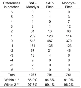
In general the ratings attributed by the three agencies are quite similar. As shown in

Table 3 around 50 per cent of all observations have the same pair-wise rating. It is also

interesting to notice that S&P and Fitch have much closer ratings, and Moody’s is more

divergent with a significant number of observations having a distance of two notches

vis-à-vis the other two agencies. This might indicate, for instance, that Moody’s and

S&P give different weights to different indicators or simply reflects the uncertainty in

measuring the default risk.

For the present study we limited the sample to 1995-2005 because of data availability of

explanatory variables. The variables inflation, unemployment, GDP growth, fiscal

balance and current account entered as a 3 years average, reflecting the agencies’

approach to take out the effect of the business cycle when deciding on a sovereign

rating. The external debt variable was taken from the World Bank and is only available

for non-industrial countries, so for industrial countries it was attributed the value 0,

which is equivalent to having a multiplicative dummy. As for the dummy variable for

European Union, we consider that the rating agencies anticipated the EU accession.

Thus we tested the contemporaneous variable as well as up to three leads. We find that

for Moody’s and S&P the variable enters with two leads, while for Fitch we find no

anticipation of EU accession. (See Appendix 1 for a full list of variables used in the

estimations as well as their specification and data sources.)

Regarding the estimation procedure, starting out with the broadest possible set of

variables, we sequentially dropped those that did not reveal any explicative power

(export growth, investment, trade openness, domestic credit growth, interest payments

(19)

4.2. Linear panel results

4.2.1. Full sample

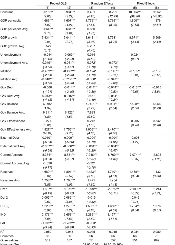
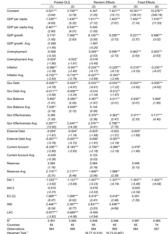
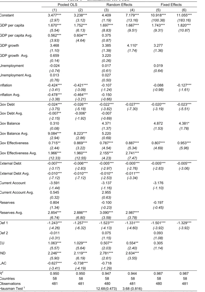
The results generated by the panel regressions point to broadly similar regression

models across the three rating agencies (see Tables 4, 5 and 6). In view of the analytical

considerations above the discussion will focus on the random effects estimations. This

is supported by the Hausmann tests reported at the end of each table pointing to the

acceptability of the random effects approach. Nevertheless, we also report the pooled

OLS and the fixed effects results for completeness and comparison purposes.

[Insert Tables 4, 5 and 6 here]

We report the results of two models for each of the rating agencies, the unrestricted and

the restricted model. While the unrestricted model incorporates all variables discussed

above, the restricted model contains only the variables which were found to have a

statistically significant impact. Although the sequence of excluding individual variables

in moving from the unrestricted to the restricted regression can have an impact on the

final specfication, the restricted models presented in the tables are quite robust to

alternative exclusion procedures. As can be seen from the statistics reported at the end

of each table, the explanatory power of the models is very high with R-square values

around 95 per cent and it remains almost constant moving from the unrestricted to the

restricted versions, while the number of observations increases marginally. In addition,

the variables found to be significant in the unrestricted model generally remain

significant with the same sign in the restricted version.

The restricted models reveal a homogenous set of explanatory variables across agencies.

On the real side, GDP per capita and GDP growth rates turn out significant for all three

companies. In the fiscal area, this applies to the government debt ratio as a difference

from the average and to the government effectiveness indicator. On the external side,

the average external debt ratio and the average level of reserves are found to be

significant across agencies. Default, EU and industrial country dummies are also

significant for all agencies. Moreover, the size of the coefficients is of the same order of

(20)

real income drive up the rating, government and external debt have a negative impact

and government effectiveness and higher external reserves have a positive impact.

Beyond this set of core variables, the agencies appear to employ a limited number of

additional variables. For Fitch the analysis finds the smallest set of additional variables,

comprising government effectiveness as a deviation from the average and foreign

currency reserves also as the short-run deviation. By contrast, the analysis finds more

significant explanatory variables for Moody’s and Standard and Poor’s, with a large

degree of homogeneity between these two agencies. In particular, on the real side

inflation is found to have a significantly negative impact. In the fiscal area, the average

debt level exerts an additional negative impact on the ratings level, whereas the fiscal

balance has a strong positive impact. With regard to the external sector, the current

account balance has a negative impact.

The findings regarding the current account effect may appear surprising as it suggests

that countries with high current account surpluses would tend to be rated lower than

otherwise equal countries without such surpluses. However, this result is quite recurrent

in the literature (Monfort and Mulder, 2000 or Eliasson, 2002). A possible explanation

is that a current account deficit could in fact serve as an indicator for the willingness of

foreigners to cover the current account gap through loans and foreign investment. In this

situation, a higher current account deficit would be associated with either higher

credit-worthiness or good economic prospects of the economy and consequently a higher

sovereign rating.

Finally, the impact of the unemployment variables appears not entirely clear cut. While

the average level of unemployment is found to have a significant negative impact on the

rating by Moody’s, the short-run deviation from the average enters positively and

significantly in the S&P model. Structural reforms that raise unemployment in the short

run but improve fiscal sustainability in the long run could provide an explanation for

this latter finding, but further research would be necessary to validate this hypothesis.

One can also assess how successfull and important our specification is. First, most of

(21)

did not include them we would be mispecifying the model.3 Second, the models pass the

Hausman test, which sugested that the problem was entirely corrected. Furthermore, if

we look at the fixed effects estimation we can see how poor it is. Notice the estimated

constant and its significance. In general the constant captures the middle rating, while

the estimated country dummies (ommited here), which vary from -7 to 7 notches,

capture each country’s average rating. All the other variables only capture small

movements from the rating in relation to its average4.

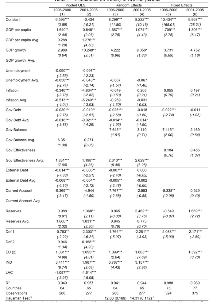
4.2.2. Differentiation across sub-periods

The separation of the overall sample into two sub-periods allows to assess broadly the

robustness of the empirical models and provides additional insight into possible changes

in the rating determinants. In particular, cutting the sample period in 2000 could reveal

any changes in the sovereign ratings methodology in response to the Asian crisis which

was perceived by market participants as revealing previously underestimated risks to

sovereign sustainability. Additionally, this also divides the full sample in two rather

similar sized sub-samples.

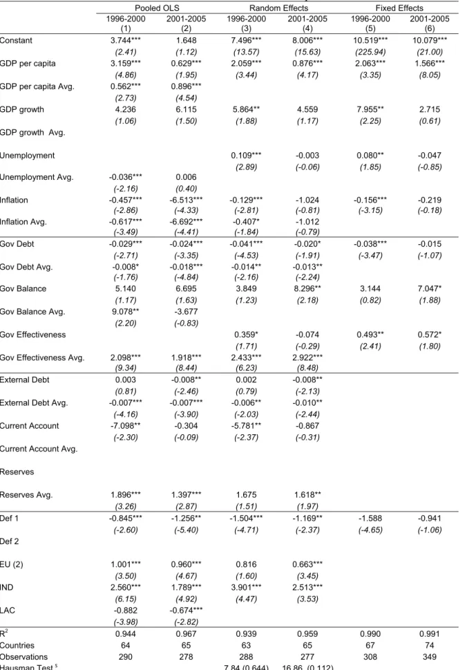
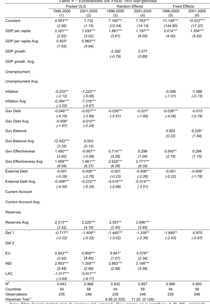
The models for the sub-periods are generally in line with those for the full estimation

period, although the significance levels of the individual coefficients are reduced (see

Tables 7–9). The lower significance levels reflect the reduction in the respective sample

sizes in half, which makes the coefficient estimates less certain. Taking this into

account, signs and orders of magnitude of the coefficient estimates from the full-period

models are mostly confirmed for the sub-periods. In particular, the core variables

identified above enter the models for the sub-periods with the correct sign and generally

significantly with a comparable order of magnitude.

Regarding the possible impact of the Asian crisis on ratings approaches, the stability of

the ratings models suggests that there was no fundamental change in methodologies. A

3_{This is in fact the cause why without including time-averages the models would not pass the Hausman}

test.

4

(22)

change that may point to some adaptation of ratings methods in response to the Asian

events is the decline in importance of the current account variable for Moody’s and

S&P, both with regard to the value of the estimated coefficient as well as its

significance level. The change may suggest that the function of the current account as

an indicator for foreigners’ willingness to cover the current account gap has declined.

Finally, for Moody’s the increase in value and significance of the coefficient on external

reserves may point to a higher importance attached to this variable after the Asian crisis.

Taken together with the reduced importance of the current account, this could suggest a

move towards a broader view on foreign financial relationships, which includes capital

flows in addition to the current account movements.

Looking at the individual agencies, for Fitch coefficient values remain remarkably

stable over the sub-periods. An exception is the negative (though insignificant) value for

GDP growth in the early sub-sample. For S&P, sign reversals between sub-periods

occur for the explanatory variables unemployment, government effectiveness and

external debt, but there are no significant coefficient estimates with opposing signs. For

Moody’s, the models point to a sign reversal for the insignificant estimate of the

coefficient on inflation.

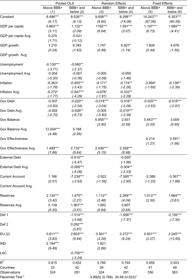
4.2.3. Differentiation across ratings levels

As a further test of the robustness of the results derived above, the sample was split into

two groups according to the ratings level: regressions were run separately for high-rated

countries with grades BBB+ and below and those above this grade. The choice of the

threshold reflects practical considerations. While market participants generally divide

bond issuers into investment-grade and non-investment grade at the threshold of BBB-,

this threshold would result in a relatively small number of observations for low ratings

making inference problematic. From the estimation of the ratigns above BBB+, we

removed the variable external debt because there were too few observations of

non-industrial countries.

The results for the separate regressions according to ratings levels confirm the overall

results from the full sample (see Tables 10–12). Looking at the random effects

(23)

agencies in the full sample also show up consistently with the correct sign in the

individual regression models for high and low ratings. Most of the coefficients are

statistically significant. Notably, the importance of average external reserves appears to

rise for low ratings in the models for Fitch and S&P. In the cases of statistical

significance external reserves always have a positive impact on the ratings.

The explanatory power of the individual regressions is somewhat lower than that found

for the full sample as well as for the sub-periods. This reflects the fact that splitting the

sample in this way reduces the number of rating categories for each estimation, so that,

with a discrete dependent variable, estimated rating errors become relatively larger.

Beyond the core variables, the results for Moody’s and S&P suggest a significant

difference in the importance of inflation for high and low ratings, respectively. For both

agencies the (significant) coefficient on inflation as an average and the deviation from it

is much higher for high ratings than for low ratings. (For Fitch, this finding is supported

by the pooled OLS and the fixed effects estimations, but not for the random effects

specification.) This suggests that for high rated countries inflation has a much more

important impact on the rating. A possible explanation is that for this set of countries

price level stability may be taken as an indicator for sound economic and in particular

monetary policies which support the long-run sustainability of government finances.

Turning to differences across agencies, the results point to a relatively high level of

consistency in the approach to high and low ratings for Fitch and Moody’s. For these

two agencies signs and (mostly) significance levels of coefficient are generally

consistent for high and low ratings. A somewhat higher degree of variation in this

regard can be observed for S&P where the sign of the estimated impact of some

variables switches between high and low ratings, although in most instances the

comparison involves statistically insignificant coefficients. Additionally, one notices

(24)

4.3. Ordered probit results

In view of the discussion of econometric issues above, ordered probit models should

give additional insight into the determinants of sovereign ratings. In particular, this

method allows to relax the rigid assumption on the shape of the ratings schedule.

Instead it generates estimates of the threshold values between rating notches allowing an

assessment of the shape of the ratings curve. Given the data requirements, the method

was only applied to the full sample, which appears appropriate in view of the overall

robustness of the empirical results to the use of sub-samples.

The results from the ordered probit estimation validate the findings highlighted above

(see Tables 13 and 14, respectively for the ordered probit robust standard errors and the

random effects ordered probit). The core variables identified in the linear regressions

also show up with the correct sign in the ordered probit approach. In addition, the

ordered probit models suggest the significance of somewhat more explanatory variables,

namely inflation and the current account, which were significant only in some

specifications in the linear approach. At the same time, in the area of external variables,

reserves do not show up significantly for Moody’s and Fitch in the restricted

specifications, both for the ordered probit and for the random effects ordered probit.

Finally, for the current account variable, the restricted specification for Moody’s shows

a negative sign for deviations from the long-term average, but a positive sign for the

average, and similar sign switches appear also in some instances for the other agencies.

This result goes some way in reconciling the counter intuitive result of the negative

effect of current account on sovereign ratings, with the conventional wisdom.

[Insert Tables 13 and 14 here]

The estimated threshold coefficients reported in the second part of the tables suggest

that the linear specification assumed for the panel regression above is appropriate. The

plot of the results of the random effects ordered probit (see Figure 2), shows that for all

three agencies the thresholds between rating notches are broadly equally distributed

across the ratings range. In other words, the distance for a country to move e.g. from B–

to B is roughly equal to that for moving from AA to AA+. Nevertheless, the

(25)

model of Moody’s, the test does not reject the null hypothesis of equal distances

between thresholds, but the significance level is close to 10 per cent. Indeed the

estimated thresholds point to a relatively large jump between the ratings for BBB– and

BBB. This suggests that countries close to the non-investment grade rating are given a

wider range before they actually cross that threshold. For Fitch, the hypothesis of equal

distances is strongly rejected as the thresholds for higher ratings are further apart than

those of the lower ratings. In this case the kink lies at the A rating.

Finally, for S&P, different distances are found throughout the ratings scale. Looking at

Figure 2, it appears that for lower ratings the relative distance between thresholds of

S&P coincides with that of Moody’s. However, above the investment grade limit, the

distances between thresholds at first decline and then increase, resulting in a slightly

curved ratings schedule that makes the transition to the highest grades most difficult.

4.4. Prediction analysis

Our prediction analysis will focus on two elements: the prediction for the rating of each

individual observation in the sample, as well as the prediction of movements in the

ratings through time.

Prediction with the pooled OLS model was done by rounding the fitted value (which is

continuous) to the closest integer between 1 and 17. For the random effects estimations

we can have two predictions, with or without the country specific effect, εi, and we can

write the corresponding estimated versions of (4) as:

ˆ ˆ ˆ

ˆ ₍ _{X )}_i _X_i _ˆ

it it i i

R =β X − +δ +λZ +ε , (7a)

ˆ₍ _{X )}_i ˆ_X_i ˆ

it it i

R% =β X − +δ +λZ . (7b)

We can then estimate each country specific effect by taking the time average of the

(26)

additional information that comes out of the estimation. In other words, we generate

in-sample and out-of-in-sample prediction. After the fitted value is computed it is then also

rounded to the closest integer between 1 and 17. The prediction with both ordered probit

and the random effects ordered probit was done by fitting the value of the latent

variable, setting the error term to zero, and then match it up to the cut points do

determine the predicted rating. Table 15 presents an overall summary of the prediction

errors, for the three agencies and for the several methods using the respective restricted

specifications.

The first conclusion is that the random effects model including the estimated country

effect is the method with the best fit. On average for the three agencies, it correctly

predicts 70 per cent of all observations and more than 95 per cent of the predicted

ratings lie within one notch (99 per cent within two notches). This is not surprising, the

country errors capture factors like political risk, geopolitical uncertainty and social

tensions that are likely to systematically affect the ratings, therefore, such term acts like

a correction for these factors.

This additional information cropping up from the random effects estimation with the

country specific effect can be very useful if we want to work with countries that belong

to our sample. But if we want to make out of sample predictions we will not have this

information. In that case, only the random effects estimation excluding the country error

is comparable to the OLS specification, to the ordered probit and to the random effects

ordered probit. We can see that in general both ordered probit and random effects

ordered probit have a better fit than the pooled OLS and random effects for all three

agencies, though not as clearly for Fitch. Overall, the simple ordered probit seems the

best method as far as prediction in levels is concerned as it predicts correctly around 45

per cent of all observations and more then 80 per cent within one notch.

Another interesting aspect to notice is that the OLS and the random effects

specifications are biased downward, while the ordered probit and random effects

ordered probit ones are slightly biased upward. The explanation for this turns out to be

(27)

rating for every category using the four estimation methods. We can see that both the

OLS and the random effects specifications tend to under predict actual AAA’s (Aaa)

while both ordered probit models and random effects ordered probit tend to over predict

the actual rating in the top categories, attributing many AAA’s (Aaa) to countries with

actual lower rating. In the bottom end of the rating scale the opposite happens, OLS and

random effects have a propensity to overestimate ratings that are bellow CCC+ (Caa1),

on the other hand, both ordered probit prediction errors are quite balanced.

[Insert Figures 3, 4 and 5 here]

Those figures provide some additional insights. For Moody’s, ordered probit performs

well in the bottom ratings while random effects ordered probit is better for top ratings.

Also notice that all four models have difficulty explaining the rating A3. Out of 21

observations the maximum correctly predicted is 2 (with OLS) with a substantial

number of predictions lying outside 1 notch.

For S&P the ordered probit outperforms all other models in the middle and bottom

categories. For Fitch, one should mention that the number of observations used for the

random effects ordered probit is higher than the other models (because of the

non-inclusion of one of the variables), which makes comparison harder. One element we

need to highlight is the fact that there is only one observation in the category A+, which

is the possible cause for the identification of the jump in both limited dependent

variable estimations, mentioned before in section 4.4. For completeness, Figure 6

reports the map of predicted ratings using the random effects estimation including

country specific errors.

Let’s now turn to how the models perform in predicting changes in ratings. Table 16

presents the total number of sample upgrades (downgrades), the predicted number of

upgrades (downgrades) and the number of upgrades (downgrades) that where correctly

predicted by the several models.

(28)

Roughly the models correctly predict between one third and one half of both upgrades

and downgrades. In our opinion this is quite satisfactory given that the empirical

approach used here necessarily neglects two sources of information that are known to

enter the decision of the rating agencies. First, in contrast to the backward-looking

models presented above, rating agencies base their decision to a considerable extent on

projected economic developments. Thus, a full empirical model of the agencies’

approach would need to incorporate the agencies’ expectations regarding the relevant

explanatory variables. However, as the agencies generally do not publish their

projections, any such modelling attempt would remain highly tentative. Still, the

observation that many of the actual rating changes are predicted by the models with a

lag of one or two years appears to support the relevance of this point. Second, ratings

agencies also generally make a clear point that they cover qualitative variables in

addition to quantitative data in the ratings process. While the relative importance of the

qualitative and quantitative factors that enter the ratings decision is uncertain (and might

well vary across countries), rating agencies’ public statements indicate that such factors

can play an important role.5 In the models above, by contrast, the only variable

reflecting such considerations is the government effectiveness indicator and it thus

appears likely that in these models the impact of qualitative factors is under-represented.

The most noticeable difference between the models is not the number of corrected

predicted changes but the total number of predicted changes. In fact, the ordered probit

and random effects ordered probit predict significantly more changes than the OLS and

random effects counterparts. For instance, for S&P, while both OLS and random effects

predict around 79 upgrades and 50 downgrades, the ordered probit model predicts 102

upgrades and 64 downgrades.

4.5. Examples of specific country analysis

In terms of the magnitude of the coefficients, the comparison between the ordered probit

and random effects ordered probit is not straightforward because the estimated distances

between the categories are different. But in general, once this is accounted for, by

5

(29)

standardising the coefficients in relation to the average jump, they are both in line with

the linear panel results. An improvement of 2 percentage points in the budget deficit, a

reduction of 5 percentage points in public debt, or a higher GDP growth by 3 percentage

points, all have the same relative impact on the ratings between 0.1 and 0.2 notches. An

increase of 10 per cent in GDP per capita would improve the rating by 0.15 to 0.25

notches. As we mentioned, a reduction of the unemployment only affects the rating if

this reduction is sustainable. If that is the case, a reduction of 4 percentage points

increases the rating by 0.2 to 0.35 notches. The effect of inflation is quite small, a

reduction of 20 percentage points on inflation increases the rating by 0.05 to 0.1

notches. These values are too small to be noteworthy for industrial countries, but if one

does the same calculation with the value estimated for high rated countries a reduction

of 4 percentage points in inflation would increase the rating by 0.15 notches.

Now that we have an idea of the estimated impact of the variables we can do some

specific country analysis. As an example, in Table 17 we show the rating for some

European countries and some emerging markets both in 1998 and 2005. Then, we use

the estimated short-run coefficients of the random effects ordered probit together with

the values for the relevant variables. Afterwards, we divide the overall prediction

change in the rating for each agency into the contributions of the different blocks of

explanatory variables: macroeconomic performance, government and fiscal

performance, external elements and European Union6_{. The upper and lower bound}

presented are computed by adding and subtracting one standard deviation to the point

estimate of the coefficients.

Let’s compare, for instance, Portugal and Spain. In 1998 they both had an AA (Aa2)

rating but in 2005 while Spain had been upgraded to AAA (Aaa) by all agencies,

Portugal had been downgraded by S&P. If we analyse the contributions of the main key

variables we see that, for Portugal the positive contribution of the macroeconomic

performance was overshadowed by the negative government developments. For such

6_{As an exception, we used the long-run coefficient of unemployment instead of the short-run coefficient.}

(30)

government performance contributed the worsening of the budget deficit since 2000, the

upward trend in government debt and the worsening in the World Bank governance

effectiveness indicator. As for Spain, the good macroeconomic performance was the

main cause of the upgrade, specially the reduction of structural unemployment since the

mid nineties and the increase of GDP per capita due to the persistent high growth.

Another example can be seen with the new European Union member states Slovakia,

the Czech Republic, Hungary, Slovenia and Poland, which have in general been

upgraded by the three agencies, in some cases more than two notches. The good

macroeconomic performance, especially in Slovakia and the Czech Republic, plays a

major role, but there was also an important credibility effect of joining the European

Union, mostly visible for Moody’s. It is in fact for Moody’s that we observe the

strongest upgrades. For Poland, the effect of the macro performance might be

undervalued. One of the key elements was the sharp reduction of inflation of more then

12 percentage points, but, as we mentioned before, the effect of inflation for high rated

countries is under assessed in the main estimations. If we consider such information,

one would have an estimated additional impact of almost half a notch.

As a final example for the emerging economies, we report the results for five countries

that have, in general also been upgraded: Brazil, Mexico, Malaysia, Thailand and South

Africa. We should briefly highlight that for Brazil the main positive contribution came

from the external area specially the reduction of external debt and the increase in

foreign reserves. This effect is particular to Fitch. For Malaysia and Thailand the main

contribution came from the macro side, while for Mexico and South Africa the

contributions are more balanced.

5. Conclusion

In this paper we studied the determinants of global sovereign debt ratings using ratings

from the three main international rating agencies, for the period 1995-2005. Overall, our

results point to a good performance of the estimated models, across agencies and across

(31)

Regarding the methodological approach, we used both a linear framework and an

ordered probit approach. We modelled the country specific error using a random effects

approach, which in practical terms implied adding time-averages of the explanatory

variables as additional time-invariant regressors. This setting allowed us to distinguish

between immediate and long-run effects of a variable on the sovereign rating level.

Moreover, we also used a limited dependent variable framework by means of an ordered

probit and random effects ordered probit specifications. The latter is the best procedure

for panel data as it considers the existence of an additional normally distributed

cross-section error term. This approach allowed both to determine the cut-off points

throughout the rating scale as well as assessing whether a linear quantitative

transformation of the ratings is actually more appropriate than a possible non-linear

transformation.

Our main findings in the panel random effects framework allowed us to detect a set of

core variables that are relevant for the determination of the ratings: per capita GDP;

GDP real growth rate; government debt; government effectiveness; external debt and

external reserves; sovereign default indicators. Moreover, the importance of fiscal

variables appears stronger than in the previous existing literature.7

The ordered probit analysis confirmed the overall estimation results from the linear

panel regressions. Interestingly, there is some evidence for different approaches of the

agencies with regard to the distance between ratings thresholds. For instance, for

Moody’s the estimated thresholds point to a relatively large jump between the ratings

for BBB– and BBB. This suggests that countries close to the non-investment grade

rating are given a wider range before they actually cross that threshold. For Fitch, the

hypothesis of equal distances is strongly rejected as the thresholds for higher ratings are

further apart than those of the lower ratings. In this case the kink lies at the A rating. On

the other hand, no clear switching pattern emerges for S&P.

The panel sample we used is quite comprehensive, which allowed for a sub-period

analysis and for a differentiated high and low rating analysis. While the results are

7_{We performed additional analysis from some different perspectives. For instance, we used the}

(32)

roughly stable across agencies, time periods and ratings levels, some additional

interesting results emerge. For instance, for the low rating levels, external debt and

external reserves are more relevant. On the other hand, for the early sub-period,

1996-2000, the current account balance was more important, while external reserves were

possibly somewhat more important in the later period, 2001-2005 (for Moody’s and

S&P). Moreover, after the Asian crisis, it seems there was a decline in the relevance of

the current account variable in the specifications for Moody’s and S&P.

Another relevant outcome ot the analysis ist that low ratings levels are more affected by

external debt and external reserves while inflation plays a bigger role for high rating

levels. On the other hand, the specifications for the Fitch ratings seem to be most

consistent over time and ratings categories. There was more variation for S&P and

Moody’s in the middle of the rating scales, which possibly points to a more quantitative

model-based approach for Fitch.

Finally, regarding the prediction analysis, the random effects model including the

estimated country effect turns out to be the method with the best fit. On average for the

three agencies, such specification correctly predicted 70 per cent of all observations and

more than 95 per cent of the predicted ratings lay within one notch. Moreover, the

models also correctly predicted between one third and one half of respectively upgrades

and downgrades. This is quite satisfactory for two reasons: first, the rating agencies also

have a forward looking behaviour that is absent from our models and second, other

qualitative factors not captured in our variables may play an important role.

Looking forward, further studies could investigate how to capture agencies’

expectations in empirical models as well as their views on qualitative variables.

Moreover, in our modelling approach we only use the government effectiveness

indicator in order to asses the impact of qualitative factors on the rating determination.

Therefore, other qualitative information could also be tentatively assessed as for

(33)

References

Afonso, A. (2003). Understanding the determinants of sovereign debt ratings: evidence

for the two leading agencies. Journal of Economics and Finance, 27 (1), 56-74.

Alexe, S.; Hammer, P.; Kogan, A. and Lejeune, M. (2003). A non-recursive regression model for country risk rating. Rutcor Research Report 9, Rutgers Center for Operational Research, March.

Bissoondoyal-Bheenick, E. (2005). An analysis of the determinants of sovereign ratings. Global Finance Journal, 15 (3), 251-280.

Bissoondoyal-Bheenick, E.; Brooks, R. and Yip, A. (2005). Determinants of sovereign ratings: A comparison of case-based reasoning and ordered probit approaches. Monash Econometrics and Business Statistics Working Papers 9/05, Monash University, Department of Econometrics and Business Statistics, May.

Borio, C. and Packer, F. (2004). Assessing new perspectives on country risk. BIS

Quarterly Review, BIS, December, 47-65.

Butler, A. and Fauver. L. (2006). Institutional Environment and Sovereign Credit

Ratings. Financial Management (forthcoming).

Cantor R. and Packer, F. (1996). Determinants and impact of sovereign credit ratings.

Economic Policy Review, 2, 37-53. Federal Reserve Bank of New York.

Canuto, O.; Santos, P. and Porto, P. (2004). Macroeconomics and Sovereign Risk Ratings, Januray, mimeo.

Eliasson, A. (2002). Sovereign credit ratings. Working Papers 02-1, Deutsche Bank.

Fitch Ratings (2006). Fitch sovereign ratings transition and default study.

Frechette, G. (2001a). sg158: Random-effects ordered probit, Stata Technical Bulletin

59, 23-27. Reprinted in Stata Technical Bulletin Reprints 10, 261-266.

Frechette, G. (2001b). sg158.1: Update to random-effects ordered probit, Stata

Technical Bulletin 61, 12. Reprinted in Stata Technical Bulletin Reprints 10, 266-267.

Hajivassiliou, V. (2006). A Modified Random Effects Estimator for Panel Data Models

with Correlated Regressors, mimeo.

Hajivassiliou, V. and Ioannides, Y. (2006). Unemployment and Liquidity Constraints.

Journal of Applied Econometrics (forthcoming).

(34)

Jaimovich, D. and Panizza, U. (2006). Public Debt around the World: A New Dataset of Central Government Debt. Working Papers 1019, Inter-American Development Bank, Research Department.

Monfort, B. and Mulder, C. (2000). Using credit ratings for capital requirements on lending to emerging market economies - possible impact of a new Basel accord. IMF Working Papers 00/69.

Moody’s (2006). Default and Recovery Rates of Sovereign Bond Issuers 1983-2005.

(available at http://www.moodys.com).

Standard & Poor’s (2004). Sovereign Defaults Set to Fall Again in 2005. (available at

http://www2.standardandpoors.com).

Standard & Poor’s (2006). 2005 Transition Data for Rated Sovereigns. (available at

http://www2.standardandpoors.com).

Rabe-Hesketh, S.; Pickles, A. and Taylor, C. (2000). sg120: Generalized linear latent

and mixed models. Stata Technical Bulletin 53, 47-57. Reprinted in Stata Technical

Bulletin Reprints 9, 293-307.

Reisen, H. and Maltzan, J. (1999). Boom and Burst and Sovereign Ratings. International Finance, 2 (2), 273-293.

Rother, P. C. (2005). The EU Premium: Ratings Strengthened for Countries Moving Toward EMU Convergence, Moody’s Special Comment, Moody’s Investors Service, August.

Wooldridge, J. (2002). Econometric Analysis of Cross Section and Panel Data. MIT

(35)

Tables and figures

Table 1 – S&P, Moody’s and Fitch rating systems and linear transformations

Rating Linear transformations

Characterization of debt and issuer (source: Moody’s)

S&P Moody’s Fitch Scale 21 Scale 17

Highest quality AAA Aaa AAA 21 17

AA+ Aa1 AA+ 20 16 AA Aa2 AA 19 15 High quality

AA- Aa3 AA- 18 14 A+ A1 A+ 17 13 A A2 A 16 12 Strong payment capacity

A- A3 A- 15 11 BBB+ Baa1 BBB+ 14 10 BBB Baa2 BBB 13 9 Adequate payment capacity

In