G.Ciobanu, M.Koutny (Eds.): Membrane Computing and Biologically Inspired Process Calculi 2010 (MeCBIC 2010) EPTCS 40, 2010, pp. 23–38, doi:10.4204/EPTCS.40.3
of Biological Systems
Richard Banks
School of Computing Science, University of Newcastle. richard.banks@ncl.ac.uk
L. Jason Steggles
School of Computing Science, University of Newcastle. l.j.steggles@ncl.ac.uk
Multi-valued network models are an important qualitative modelling approach used widely by the biological community. In this paper we consider developing an abstraction theory for multi-valued network models that allows the state space of a model to be reduced while preserving key properties of the model. This is important as it aids the analysis and comparison of multi-valued networks and in particular, helps address the well–known problem of state space explosion associated with such analysis. We also consider developing techniques for efficiently identifying abstractions and so provide a basis for the automation of this task. We illustrate the theory and techniques developed by investigating the identification of abstractions for two published MVN models of the lysis–lysogeny switch in the bacteriophageλ.
1
Introduction
In order to understand and analyse the complex control mechanisms inherent in biological systems a range of formal modelling techniques have been applied by biologists (for an overview see for example [4, 7]). In particular, qualitative modelling techniques have emerged as an important modelling approach due to the lack of quantitative data on reaction rates and the noise associated with such data.Multi-valued networks(MVNs) [15, 18, 19] are a promising qualitative modelling approach for biological systems. They extend the well–knownBoolean networkapproach [1, 4] by allowing the state of each regulatory entity to be within a range of discrete values instead of just on/off. In this way they are able to provide a compromise between the simplicity of Boolean networks and the more detailed differential equational models.
However, the analysis of MVNs is not without problems. They suffer from the well–known state space explosion problem, a problem which is exacerbated in MVNs by the possibly large set of states associated with each individual entity. Another important shortcoming is the lack of any techniques for relating MVN models at different levels of abstraction. This hinders the comparison of MVN models and means there is no basis for the incremental development of MVNs.
We illustrate the theory and techniques developed by investigating the existence of abstractions for two published MVN models for the genetic regulatory network controlling the lysis–lysogeny switch in the bacteriophage λ [17, 5]. Bacteriophage λ [18, 14] is a virus which after infecting the bacteria
Escherichia colimakes a decision to switch to one of two possible reproductive phases. It can enter the
lytic cyclewhere the virus generates as many new viral particles as the infected cell’s resources allow and then lyse the cell wall to release the new phage. Alternatively, it can enter thelysogenic cyclewhere theλ DNA integrates into the host DNA providing it with immunity from other phages and allowing it to be replicated with each cell division. We consider a two and four entity MVN model [17] of the lysis–lysogeny switching mechanism and using the techniques we have developed identify corresponding abstractions for these models.
This paper is organized as follows. In Section 2 we provide a brief overview of the MVN modelling approach and present a simple illustrative example. In Section 3 we develop an abstraction theory for multi-valued networks and present a range of results concerning this theory. In Section 4 we consider the identification of abstractions and develop a basis for automating the abstraction process. In Section 5 we illustrate the theory and techniques developed by presenting two abstraction examples for pub-lished models of the lysis–lysogeny switch in bacteriophage λ. Finally, in Section 6 we present some concluding remarks and consider directions for future work.
2
Multi-valued Network Models
In this section, we introduce multi-valued networks (MVNs) [15, 18, 19], a qualitative modelling ap-proach which extends the well-knownBoolean network[1] approach by allowing the state of each regu-latory entity to be within a range of discrete values. MVNs have been extensively studied in circuit design (for example, see [15, 12]) and successfully applied to modelling biological systems (for example, see [19, 5, 16]).
An MVN consists of a set of logically linked entitiesG={g1, . . . ,gk}which regulate each other in
a positive or negative way. Each entitygi in an MVN has an associated set of discrete statesY(gi) =
{0, . . . ,mi}, for some mi ≥1, from which its current state is taken. Note that a Boolean network is
therefore simply an MVN in which each entitygihas a Boolean set of statesY(gi) ={0,1}. Each entity
gialso has a neighbourhoodN(gi) ={gi1, . . . ,gil(i)}which is the set of all entities that can directly affect
its state. (Note thatgi may or may not be a member ofN(gi).) Furthermore, interactions between one
entity and another only become functional if the state of the source entity has reached some threshold state level (this threshold state level is always at least one). MVNs can therefore discriminate between the strengths of different interactions, something which Boolean networks are unable to capture. The behaviour of each entitygi based on these neighbourhood interactions is formally defined by a logical
next-state function fgi which calculates the next-state ofgi given the current states of the entities in its
neighbourhood.
We can now define an MVN more formally as follows.
Definition 1. An MVNMVis a four-tupleMV= (G,Y,N,F)where:
i)G={g1, . . . ,gk}is a non-empty, finite set of entities;
ii)Y = (Y(g1), . . . ,Y(gk))is a tuple of state sets, where eachY(gi) ={0, . . . ,mi}, for somemi≥1, is the
state space for entitygi;
iii)N= (N(g1), . . . ,N(gk))is a tuple of neighbourhoods, such thatN(gi)⊆Gis the neighbourhood of
iv)F = (fg1, . . . ,fgk) is a tuple of next-state multi-valued functions, such that if N(gi) ={gi1, . . . ,gin}
then the function fgi :Y(gi1)× · · · ×Y(gin)→Y(gi)defines the next state ofgi. ✷
In the sequel, letMV= (G,Y,N,F)be an arbitrary MVN. In a slight abuse of notation we letgi∈MV
represent thatgi∈Gis an entity inMV.
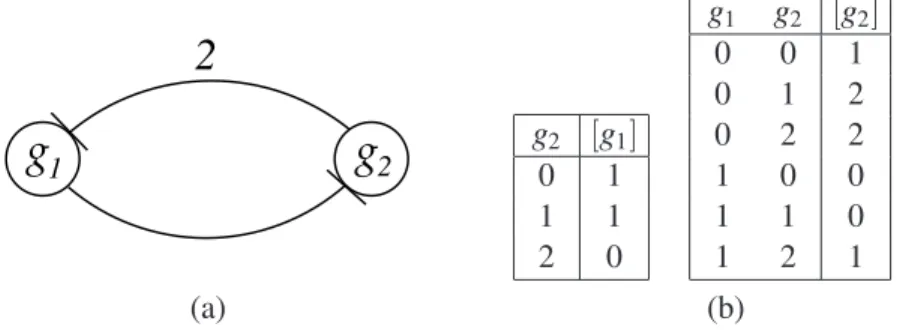
As an example, consider the MVNEx1 defined in Figure 1 which consists of two entitiesg1andg2,
such thatY(g1) ={0,1}andY(g2) ={0,1,2}. The update functions for each entity are defined using
state transition tables (see Figure 1.(b)) where[gi]is used to denote the next state of an entitygi. It can
be seen that entityg1 inhibitsg2 and that entity g2 inhibitsg1 but only when it reaches state 2 (this is
represented in Figure 1.(a) by labelling the corresponding edge with a 2). Note that althoughg2∈N(g2)
we have not drawn an edge for this in Figure 1.(a) sinceg2has no regulatory affect on itself and is needed
simply to allow the affect ofg1to be precisely defined.
2
g
g
1 2g2 [g1]
0 1
1 1
2 0
g1 g2 [g2]
0 0 1
0 1 2
0 2 2
1 0 0
1 1 0
1 2 1
(a) (b)
Figure 1: An example MVN Ex1 which consists of two entities g1 and g2, including: (a) network
structure; and (b) the state transition tables representing the corresponding next-state functions.
Aglobal state of an MVNMVwithk entities is represented by a tuple of states(s1, . . . ,sk), where
si∈Y(gi)represents the state of entitygi∈MV. Note as a notational convenience we often uses1. . .skto
represent a global state(s1, . . . ,sk). When the current state of an MVN is clear from the context we allow
gi to denote both the name of an entity and its corresponding current state. The state space of an MVN
MV, denotedSMV, is therefore the set of all possible global statesSMV=Y(g1)× · · · ×Y(gk). The state of
an MVN can be updated eithersynchronously, where the state of all entities is updated simultaneously in a single update step, orasynchronously, where entities update their state independently (see [9]). In the following we focus on the synchronous update semantics since this has received considerable attention from the biological community. Given two states S1,S2 ∈SMV, let S1→S2 represent a synchronous
update stepsuch thatS2 is the state that results from simultaneously updating the state of each entitygi
using its associated update function fgi and the appropriate neighbourhood of states fromS1.
As an example, consider the global state 01 forEx1 (see Figure 1) in which g1 has state 0 andg2
has state 1. Then 01→12 is a single synchronous update step on this state resulting in the new state 12. The sequence of global states throughSMVfrom some initial state is called atrace. Note that in the case
of a synchronous update semantics such traces are infinite. However, given that the global state space is finite, this implies that a trace must eventually enter a cycle, known formally as an attractor cycle
[11, 19]. We make use of this fact to define a finite canonical representation for traces which specifies a trace up to the first repeated state.
Definition 2. Let S0 ∈SMV be a global state for MV. A trace is a list of global states σ(S0) =
i)Si→Si+1, for 0≤i<n;
ii)S0, . . . ,Sn−1are unique states; and
iii)Sn=Sifor somei∈ {0, . . . ,n−1}. ✷
The set of all tracesTr(MV) ={σ(S)|S∈SMV}therefore completely characterizes the behaviour of
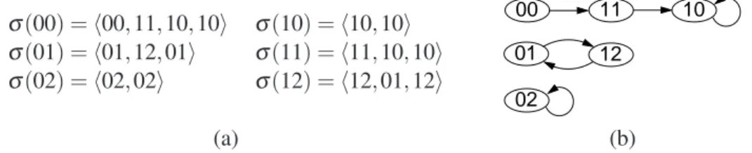
an MVN model under the synchronous semantics and is referred to as thetrace semanticsofMV. In our running example,Ex1 has a state space of size|SEx1|=6 and so (under a synchronous update
semantics)Tr(Ex1)consists of the six traces presented in Figure 2.(a) below.
σ(00) =h00,11,10,10i σ(10) =h10,10i
σ(01) =h01,12,01i σ(11) =h11,10,10i σ(02) =h02,02i σ(12) =h12,01,12i
00 11 10
01
02
12
(a) (b)
Figure 2: The trace semantics forEx1: (a) the set of formal traces; and (b) a graphical representation of the traces.
As mentioned above, each trace leads to a cyclic sequence of states known as an attractor cycle
[11, 19]. For example, in Figure 2.(b) we can see thatEx1 has three attractors: 10→10 and 02→02 known aspoint attractors; and 01→02→01 which is an attractor cycle of period 2 [11].
Given a trace σ =hS1, . . . ,Sni ∈Tr(MV) for an MVNMVwe let att(σ)denote the attractor cycle
that must occur in traceσ, i.e. att(σ) =hSk, Sk+1, . . . ,Sni, for some 1≤k<nand Sk =Sn. We let
ATT(MV)denote the set of all attractors forMV, i.e.
ATT(MV) ={att(σ)|σ ∈Tr(MV)}.
Attractor cycles are very important biologically where they are seen as representing different biolog-ical states or functions (e.g. different cellular types such as proliferation, apoptosis and differentiation [10]). Thus, the identification and analysis of attractor cycles for MVNs is an important subject which has warranted much attention in the literature (for example, see [11, 19, 8]).
3
An Abstraction Theory for MVNs
In this section we develop a notion of abstraction for MVNs by considering what it means for one MVN to abstractly implement the behaviour of another. This is based around the idea of showing that the trace semantics of one MVN is consistent with the trace semantics of a more complex MVN under an appropriate mapping of states.
We begin by defining how an entity’s state space can be simplified using a mapping to merge states.
Definition 3. LetMVbe an MVN and letgi ∈MVbe an entity such thatY(gi) ={0, . . . ,m}for some
m>1. Then astate mappingφ(gi)for entitygiis a surjective mappingφ(gi):{0, . . . ,m} → {0, . . . ,n},
where 0<n<m. ✷
used. Note we only consider state mappings with a codomain larger than one, since a singular state entity does not appear to be of biological interest.
As an example, consider entityg2∈Ex1 (see Figure 1) which has the state spaceY(g2) ={0,1,2}. It
is only meaningful to simplifyg2∈Ex1 to a Boolean entity and so one possible state mapping to achieve
this would be:
φ(g2) ={07→0,17→0,27→1},
which merges states 0 and 1 into a single state 0, and translates state 2 into 1.
Clearly, there are a number of different possible state mappings which can be applied to reduce a node’s state space from mton states, for 1<n<m. The complete set of all such state mappings is
denotedMS(m,n) ={φ |φ :{0, . . . ,m−1} → {0, . . . ,n−1}and φ is sur jective}. For example, the mapping setMS(3,2)consists of the following six mappings:
(1) {07→0,17→0,27→1} (4) {07→1,17→1,27→0} (2) {07→0,17→1,27→1} (5) {07→1,17→0,27→0}
(3) {07→0,17→1,27→0} (6) {07→1,17→0,27→1}
In order to be able to consider simplifying several entities at the same time during the abstraction process we introduce the notion of a family of state mappings as follows.
Definition 4. LetMV= (G,Y,N,F)be an MVN with entities G={g1, . . . ,gk}. Then anabstraction
mappingφ forMVis a family of mappingsφ =hφ(g1), . . . ,φ(gk)isuch that for each 1≤i≤kwe have
φ(gi)is either a state mapping for entitygior is the identity mappingIgi:Y(gi)→Y(gi)whereIgi(s) =s,
for alls∈Y(gi). Furthermore, forφ to be well–defined we insist that at least one of the mappingsφ(gi)
is a state mapping. ✷
Note in the sequel given a state mapping φ(gi) we let it denote both itself and the corresponding
abstraction mapping containing only the single state mappingφ(gi).
An abstraction mapping can be lifted and applied to the trace semantics of an MVN as follows.
Definition 5. An abstraction mappingφ =hφ(g1). . .φ(gk)ifor MVcan be used to abstract a global
states1. . .sk ∈SMV by applying it pointwise, i.e. φ(s1. . .sk) =φ(g1)(s1). . .φ(gk)(sk). We can lift an
abstraction mappingφto a traceσ(S0) =hS0, . . . ,Sni ∈Tr(MV)by applyingφto each global state in the
trace as follows
φ(σ(S0)) =hφ(S0), . . . ,φ(Sn)i.
However,φ(σ(S0))may contain contradictory steps and thus not represent a meaningful abstracted trace.
We say an abstracted traceφ(σ(S0))isvalid iff there does not exist two identical statesφ(Si) =φ(Sj),
for somei,j∈ {0, . . . ,n−1}, such thatφ(Si+1)6=φ(Sj+1). Ifφ(σ(S0))is a valid abstracted trace then
we need to ensure it is in the canonical form introduced in Definition 2. We do this by removing any repeating tail that may have been introduced by the abstraction mapping, i.e. choose the smallest k, 0<k≤nsuch thatφ(S0), . . . ,φ(Sk−1)are unique states andφ(Si) =φ(Sk), for somei∈ {0, . . . ,k−1}.
(Note whenever we talk about a valid abstracted trace we will assume it is in its canonical form.) We can liftφto the trace semantics of a modelMV:
φ(Tr(MV)) ={φ(σ(S))|σ(S)∈Tr(MV)andφ(σ(S))is valid}.
Continuing with our running example, φ(g2)can be applied as an abstraction mapping to the trace
semantics Tr(Ex1) (see Figure 2) resulting in the abstracted trace semantics φ(g2)(Tr(Ex1)), shown
below in Figure 3, in which the states ofg2have been reduced accordingly.
φ(g2)(σ(00)) =h00,10,10i φ(g2)(σ(10)) =h10,10i
φ(g2)(σ(01)) =h00,11,00i φ(g2)(σ(11)) =h10,10i
φ(g2)(σ(02)) =h01,01i φ(g2)(σ(12)) =h11,00,11i
Figure 3: The trace semanticsφ(g2)(Tr(Ex1))resulting from abstractingTr(Ex1)usingφ(g2).
Note thatφ(g2)(Tr(Ex1))is non–deterministic in the sense that we have two different traces
begin-ning with the same state 00 (i.e. starting in state 00 we have a non-deterministic choice between two abstracted traces,h00,10,10i andh00,11,00i). This occurs as we are viewing the more complex set of behaviours captured byTr(Ex1)from a simpler perspective.
To illustrate how invalid abstracted traces arise consider an MVN with two entities that has the following trace σ(00) =h00,11,01,02,02i. When σ(00) is abstracted with the standard abstraction mappingφ(g2) ={07→0,17→0,27→1}the result is the following
φ(g2)(σ(00)) =h00,10,00,01,01i.
However, it can be observed that this is not a valid trace according to Definition 5 because global state 00 can lead to two different states and will therefore be omitted from the abstracted trace semantics.
We are now ready to define what it means for one MVN to be an abstraction of another.
Definition 6. Let MV1= (G1,Y1,N1,F1) and MV2= (G2,Y2,N2,F2) be two MVNs with the same
structure, i.e. G1=G2 and N1(gi) =N2(gi), for all gi∈MV1. Letφ be an abstraction mapping from
MV2 to MV1. Then we say that MV1 abstracts MV2 under φ, denoted MV1✁φMV2, if, and only if,
Tr(MV1)⊆φ(Tr(MV2)). ✷
An abstraction MV1✁φMV2 indicates that the model MV1 consistently abstracts the behaviour of
a more complex modelMV2 by reducing the state space of those entities identified in the abstraction
mappingφ. Note alternatively, we could considerMV2to be arefinementofMV1in the sense thatMV2
consistently extendsMV1with the addition of further states. Such a notion of refinement is useful as it
provides a framework for the incremental development of MVN models.
As an abstraction example, consider the MVNEx2 defined in Figure 4 which has the same structure asEx1 (see Figure 1) but is a Boolean model. Then clearly, given the abstraction mappingφ(g2)
intro-g2 [g1]
0 1
1 0
g1 g2 [g2]
0 0 1
0 1 1
1 0 0
1 1 0
σ(00) =h00,11,00i
σ(01) =h01,01i σ(10) =h10,10i σ(11) =h11,00,11i
Figure 4: State transition tables definingEx2 and its associated trace semanticsTr(Ex2).
duced earlier, we can see thatTr(Ex2)⊆φ(g2)(Tr(Ex1))holds and soEx2 is an abstraction ofEx1, i.e.
In special cases, an abstraction may exactly capture the behaviour of the original MVN model under the given abstraction mapping. We distinguish this stronger case with the notion of anexact abstraction.
Definition 7. Let MV1 and MV2 be two MVNs such that MV1✁φMV2 for some abstraction
map-pingφ. Then we say thatMV1 exactly abstracts MV2under φ, denoted MV1=φ MV2, if, and only if,
Tr(MV1) = φ(Tr(MV2))and for everyσ∈Tr(MV2), the abstracted traceφ(σ)is valid. ✷
Exact abstractions are interesting as they indicate redundant states (normally corresponding to en-tity thresholds) which have no affect on the qualitative behaviour of an MVN. Subsequently, an exact abstraction provides a simpler representation of an MVN whilst preserving all its behaviour under the given abstraction mapping.
It is natural to consider whether every (non–Boolean)1 MVN has an abstraction. In other words, do there exist MVNs which contain regulatory interactions which are too subtle to be represented in a sim-pler state domain. This is an interesting question since it provides insight into the need for non-Boolean MVN models. Unsurprisingly, it turns out that abstractions do not always exist, as formalized in the following theorem.
Theorem 8. Not every non–Boolean MVN has an abstraction.
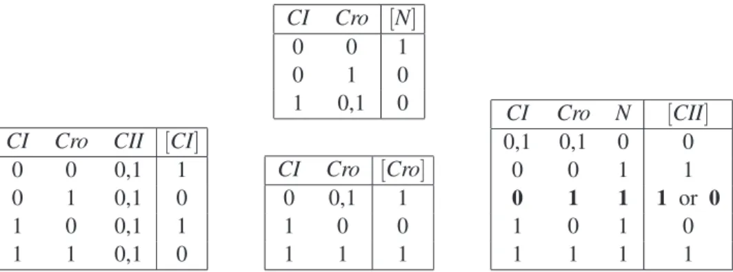
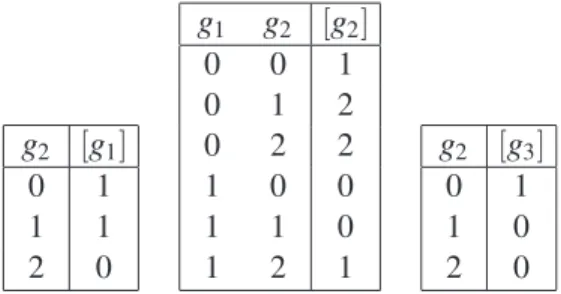
Proof. We simply construct a non–Boolean MVN which we show has no abstractions. Let Ex3 be
defined by extending Ex1 (Figure 1) with a third Boolean entity g3 which is inhibited wheneverg2 is
in a state greater than or equal to 1. The complete definition forEx3 is given in Figure 5. We can see
g2 [g1]
0 1
1 1
2 0
g1 g2 [g2]
0 0 1
0 1 2
0 2 2
1 0 0
1 1 0
1 2 1
g2 [g3]
0 1
1 0
2 0
Figure 5: The state transition tables definingEx3 (used to prove Theorem 8).
thatg2∈Ex3 now acts in two subtly different ways: on one handg1 is inhibited wheng2=2; and on
the other hand, g3 is inhibited wheng2≥1. We can show that no abstraction exists for this model by
exhaustively considering each possible abstraction mappingφ(g2) and showing that for every possible
candidate abstraction modelMVAwe haveTr(MVA)6⊆φ(g2)(Tr(Ex3)). ✷
This is an important result which, although centered around the relationship assumption formalized by our abstraction theory, provides insight into the expressive power of MVNs and in particular, motivates the need for multi-valued modelling techniques.
One of the main motivations for defining an abstraction theory is to allow simplified models of an MVN to be identified to aid the analysis process. This therefore raises the question of what properties of an abstraction are preserved by the original MVN and we end this section by considering this question.
We begin by introducing a notion of corresponding states and traces.
Definition 9. Let MV be an MVN with an abstraction MVA under a given abstraction mapping φ,
i.e. MVA✁φMV. LetSA∈SMVA be some global state of abstractionMVA andS∈SMV be a global state
of the original modelMV. Then we say thatSA and S correspond with respect toφ, denotedSA✁φS, if, and only if,SA=φ(S).Furthermore, given tracesσA∈Tr(MVA)andσ ∈Tr(MV)we sayσAand σ
correspond with respect toφ, denotedσA✁φσ, if, and only if,φ(σ)is valid andσA=φ(σ). ✷
Let S1
∗
→S2 denote the fact that global state S2 ∈SMV is reachable from global state S1∈SMV in
the modelMV. We now clarify the relationship between reachability properties in an abstraction and its corresponding original MVN model.
Theorem 10. LetMVA✁φMV for some mapping abstraction φ and let SA1,SA2 ∈SMVA. If S
A
1
∗
→SA2
inMVAthen there must exist statesS1,S2∈SMVsuch thatSA1✁φS1,SA2✁φS2, andS1→∗ S2inMV.
Proof. Since SA
1
∗
→SA
2 there must exist a traceσ(SA1)∈Tr(MVA) containing SA2. From Definition 6,
we know thatTr(MVA)⊆φ(Tr(MV))must hold. Therefore there must exist a stateS1∈SMV such that
σ(SA
1)✁φσ(S1), i.e. φ(σ(S1)) =σ(S1A). From this it is straightforward to see that there must exist the
required stateS2in traceσ(S1)such thatS2A✁φS2andS1→∗ S2. ✷
In other words, reachability properties of abstractions have corresponding reachability properties in the original MVN. However, since abstractions normally capture less behaviour than the original model, there are limitation on what can be deduced from an abstraction. It turns out that determining reachability in a model using an abstraction is a semi-decidable property: (i) By Theorem 10 we know that if one state is reachable from another in an abstraction then a corresponding reachability property must hold in the original model; (ii) However, if one state is not reachable from another in an abstraction then a corresponding reachability property in the original MVN may or may not hold and more analysis will be required.
The final result we present is important as it shows that the attractor cycles found in an abstraction are preserved by the original MVN.
Theorem 11. LetMVA✁φMVfor some abstraction mappingφ. Then
ATT(MVA)⊆φ(ATT(MV)).
Proof. Letτ∈ATT(MVA)then we need to show that τ ∈φ(ATT(MV)). By definition we know there
must exist a traceσA∈Tr(MVA) such thatatt(σA) =τ. SinceMVA✁φMVwe know there must exist
a trace σ ∈Tr(MV) such thatφ(σ) is valid and σA=φ(σ). It follows that τ =φ(att(σ))and so by
definition we know thatτ∈φ(ATT(MV))as required. ✷
4
Identifying Model Abstractions
In the previous section we defined a formal notion of what it means for one MVN to be a correct ab-straction of another. Given an MVNMVand an abstraction mappingφ we can therefore define the set
AS(MV,φ)of all abstractions ofMVunderφ, i.e.
Finding abstractions, i.e. members ofAS(MV,φ), is clearly an important task given that they provide a means of simplifying the analysis of a model and can help address the well-known problem of state space explosion. However, in practice, the brute force derivation of this refinement set becomes intractable for all but the smallest MVN. Specifically, if we havekentities each withnstates, then we have a worst case upper bound of(nnk)k possible candidate models to consider for any abstraction mapping. For instance,
there are(223)3=16777216 possible Boolean networks consisting of just three entities! The rest of this
section considers techniques for efficiently identifying abstractions and provides a basis for automating this task. Initial ideas for implementing these techniques are presented in [2].
We begin by considering how an abstraction mapping can be applied to an MVN to produce a set of potential abstraction models.
Definition 12. Let φ =hφ(g1), . . . ,φ(gk)i be an abstraction mapping for an MVN MV. For each
entitygi∈MVwe can abstract the next-state function fgi :Y(gi1)× · · · ×Y(gin)→Y(gi)to a (possibly)
non-deterministic next-state function
φ(fgi):φ(gi1)(Y(gi1))× · · · ×φ(gin)(Y(gin))→φ(gi)(Y(gi))
by applyingφto its definition in the obvious way. We say thatMVAresults from applyingφto MViff: (1)MVAhas the same entities and neighbourhood structure asMV;
(2) The state space of each entitygi∈MVAis the setφ(gi)(Y(gi));
(3) For eachgi∈MVAits next-state function fMV
A
gi :φ(gi1)(Y(gi1))× · · · ×φ(gin)(Y(gin))→φ(gi)(Y(gi))
is a deterministic restriction ofφ(fgi).
We defineφ(MV)to be the set of all such MVNs, i.e.
φ(MV) ={MVA |MVAresults from applyingφtoMV}
The trace semantics ofφ(MV)is then defined byTr(φ(MV)) =SMVA∈φ(MV)Tr(MVA) ✷
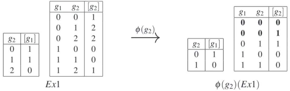
To illustrate this idea, consider applying the abstraction mapping φ(g2) ={07→0,17→0,27→1}
to the example MVNEx1 introduced in Section 2 (see Figure 1). The resulting abstracted next-state functions are presented in Figure 6. The setφ(g2)(Ex1)will contain two candidate abstractions in which
the state space forg2 is reduced to{0,1} and whose next-state functions are given by the two possible
interpretations (highlighted in bold) for the abstracted state transition table forg2given in Figure 6.
g2 [g1]
0 1
1 1
2 0
g1 g2 [g2]
0 0 1
0 1 2
0 2 2
1 0 0
1 1 0
1 2 1
φ(g2)
−→
g2 [g1]0 1
1 0
g1 g2 [g2]
0 0 0
0 0 1
0 1 1
1 0 0
1 1 0
Ex1
φ
(g2)(Ex1)Figure 6: The (non–deterministic) state transition tables for φ(g2)(Ex1) which result from applying
An interesting observation arises by noting that for a given modelMVand abstraction mapping φ, the trace semantics of the abstracted MVNTr(φ(MV))is not in general the same as the abstracted trace semanticsφ(Tr(MV)). In fact, it turns out that an important relationship exists between the two, in that
Tr(φ(MV))will always contain at least the traces ofφ(Tr(MV)), as shown by the following theorem.
Theorem 13. Letφ=hφ(g1), . . . ,φ(gk)ibe an abstraction mapping forMV. Then we have
φ(Tr(MV))⊆Tr(φ(MV)).
Proof. Letσ =hS0, . . . ,Sni ∈Tr(MV)be an arbitrary trace, then we need to show that ifφ(σ)is a valid
abstracted trace thenφ(σ)∈Tr(φ(MV)). LetSi→Si+1be an arbitrary state step inσ. AssumingMVhas
kentities then this state step can be broken up intok componentsSi→Sij+1, for j=1, . . . ,k. Applying
the abstraction mapping to each component givesφ(Si)→φ(gj)(Sij+1). Clearly, by Definition 12 there
must existMVA∈φ(MV)whose next-state functions reproduce each of these abstracted component steps and so is able to reproduce the complete abstracted state stepφ(Si)→φ(Si+1). Sinceφ(σ)is a valid
abstracted trace it follows that we must be able to findMVA∈φ(MV)which is able to reproduce all the abstracted state stepsφ(Si)→φ(Si+1), fori=0, . . . ,n−1. Thus, we knowφ(σ)∈Tr(MVA)and so by
Definition 12 we haveφ(σ)∈Tr(φ(MV))as required. ✷
From this result, it follows that any abstraction of an MVNMVmust be contained within the set of potential abstractionsφ(MV)as formalized in the corollary below.
Corollary 14. Given two MVNsMV1andMV2we have that
MV1✁φMV2 =⇒ MV1∈φ(MV2).
Proof. By Definition 6 we knowTr(MV1)⊆φ(Tr(MV2))and so by Theorem 13 we haveTr(MV1)⊆
Tr(φ(MV2)). It therefore follows by Definition 12 thatMV1∈φ(MV2). ✷
Corollary 14 provides an important necessary condition for an MVN to be an abstraction of another for a given abstraction mapping. It gives us a way of restricting the models that need to be considered when iterating through possible candidate abstractions for an MVN; we simply apply the abstraction mapping to the MVN in question and then consider each possible deterministic model that results from this application. This observation results in an exponentially smaller search space and provides the basis for a more efficient abstraction finding algorithm.
To illustrate the above ideas let us consider finding all the abstractions forEx1 underφ(g2), i.e.
cal-culating the abstraction setAS(Ex1,φ(g2)). Using the results from Corollary 14, we begin by abstracting
the state transition tables forEx1 using the given abstraction mapping (shown previously in Figure 6) and identifying the potential abstractions contained inφ(g2)(Ex1). We can see that the behaviour ofg2
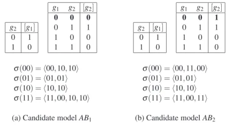
is non-deterministic wheng1=0 andg2=0. As such, we have just two possible candidate modelsAB1
andAB2to consider, shown respectively by Figure 7.(a) and Figure 7.(b) (where the rules highlighted in
bold are the only ones that differ).
In order to verify whetherAB1and AB2 are indeed abstractions according to our theory, we check
if their trace semantics are contained withinφ(g2)(Tr(Ex1)). By considering Figure 3 and Figure 7 we
can observe thatAB1 is not an abstraction according to Definition 6, sinceTr(AB1)6⊆φ(g2)(Tr(Ex1));
g2 [g1]
0 1
1 0
g1 g2 [g2]
0 0 0
0 1 1
1 0 0
1 1 0
g2 [g1]
0 1
1 0
g1 g2 [g2]
0 0 1
0 1 1
1 0 0
1 1 0
σ(00) =h00,10,10i σ(01) =h01,01i
σ(10) =h10,10i σ(11) =h11,00,10,10i
σ(00) =h00,11,00i σ(01) =h01,01i
σ(10) =h10,10i σ(11) =h11,00,11i
(a) Candidate modelAB1 (b) Candidate modelAB2
Figure 7: The state transition tables and trace semantics for candidate modelsAB1andAB2.
the same MVN asEx2 which was introduced as an abstraction in the previous section.) Thus, we have shown that the refinement set AS(Ex1,φ(gi)) = {AB2}.
It can be observed that exact refinements occur precisely when the translated MVN has a singleton set of candidate abstraction models, as shown by the following theorem.
Theorem 15. Letφbe an abstraction mapping for some MVNMV. Then we know the following:
(1) ifφ(MV) ={MVA}is a singleton set, thenMVA=φ MV;
(2) ifφ(MV)is not a singleton set, then no exact abstraction forMVcan exist underφ.
Proof. To prove (1), we observe that if φ(MV) ={MVA} is a singleton set then for each gi ∈MV
the abstracted next-state functionφ(fgi) must be deterministic. This implies that all abstracted traces
φ(σ), for σ ∈Tr(MV)must be valid. Furthermore, by Definition 12 and Theorem 13 it follows that
Tr(MVA) =φ(Tr(MV))as required.
To prove (2), note that ifφ(MV)contains more than one potential abstraction model then there must exist at least one abstracted next-state function φ(fgi) which is non–deterministic. This implies there
must exist at least one abstracted global state which leads to two or more different traces. Clearly, either some of these abstracted traces are invalid orφ(Tr(MV))must contain more traces than any single abstraction model could capture. Therefore, there cannot exist an exact abstraction forMV. ✷
5
Illustrative Biological Examples
In this section we illustrate the theory and techniques developed in the previous sections by investigating the existence of abstractions for two published MVN models for the genetic regulatory network control-ling the lysis–lysogeny switch in the bacteriophageλ [17, 5]. We begin with a brief introduction to the bacteriophageλ (see [14] for a more detailed introduction).
in the λ DNA synthesize a repressor which blocks expression of other phage genes including those involved in its own excision. As such, the host cell establishes an immunity to external infection from other phages, and the phageλ is able to lie dormant, replicating with each subsequent cell division of the host.
5.1 The Two Entity Core Regulatory Model
A simple MVN model of the core regulatory mechanism for the lysis–lysogeny switch was proposed in [17]. This model, which we denote as PL2, is presented in Figure 8 and is based on the cross– regulation between two regulatory genes, CI (the repressor gene) and Cro. It can be seen that Cro
inhibits the expression ofCI and at higher levels of expression, also inhibits itself. The geneCIinhibits the expression ofCrowhile promoting its own expression. The full synchronous trace semanticsTr(PL2)
for this MVN is presented in Figure 8.(c). We can see from the state transition graph in Figure 8.(d) that
PL2has three attractor cycles, where the attractor cycle 10→10 represents the lysogenic cycle since the repressor geneCIis fully expressed and 01→02→01 represents the lytic cycle.
2
Cro
CI
σ(00) =h00,11,00i σ(10) =h10,10i
σ(01) =h01,02,01i σ(11) =h11,00,11i σ(02) =h02,01,02i σ(12) =h12,01,02,01i
(a) Network structure (c) Trace semantics
CI Cro [CI]
0 0 1
0 1 0
0 2 0
1 0 1
1 1 0
1 2 0
CI Cro [Cro]
0 0 1
0 1 2
0 2 1
1 0 0
1 1 0
1 2 1
00 11
01 02 12
10
(b) State transition tables (d) Graphical representation of traces
Figure 8: Formal definition and trace semantics for the MVN modelPL2of the core regulatory mecha-nism for the lysis-lysogeny switch in bacteriophageλ (taken from [17]).
In order to identify an abstraction for PL2 we begin by selecting an appropriate state mapping φ(Cro):{0,1,2} → {0,1}for the only non-Boolean entityCro. We use our understanding of the be-haviour ofCroto define the following state mapping
φ(Cro) ={07→0,17→1,27→1}.
CI Cro [CI]
0 0 1
0 1 0
1 0 1
1 1 0
CI Cro [Cro]
0 0 1
0 1 1
1 0 0
1 1 0
σ(00) =h00,11,00i
σ(01) =h01,01i
σ(10) =h10,10i σ(11) =h11,00,11i
Figure 9: Abstraction modelAPL2forPL2and associated trace semanticsTr(APL2).
φ(Cro)(σ(00)) =h00,11,00i φ(Cro)(σ(10)) =h10,10i
φ(Cro)(σ(01)) =h01,01i φ(Cro)(σ(11)) =h11,00,11i φ(Cro)(σ(02)) =h01,01i φ(Cro)(σ(12)) =h11,01,01i
Figure 10: The tracesφ(Cro)(Tr(PL2))resulting from abstracting the traces ofPL2usingφ(Cro).
It can be seen that the abstractionAPL2acts as a good approximation to the behaviour of the original MVNPL2and in particular, we can see that the abstraction has captured all three attractor cycles that were present inPL2.
5.2 The Four Entity Regulatory Model
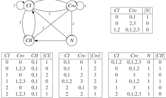
The core regulatory model presented above was extended in [17] to take account of the actions of two further regulatory genes, CIIand N. The resulting four entity MVN modelPL4is presented in Figure 11 (note that the state transition tables presented use a shorthand notation where an entity is allowed to be in any of the states listed for it in a particular row). This MVN is more detailed than PL2and
3
Cro CI
CII N
2 2
2
3 2
CI Cro [N]
0 0,1 1
0 2,3 0
1,2 0,1,2,3 0
CI Cro CII [CI]
0 0 0,1 1
0 1,2,3 0,1 0
1 0 0,1 2
1 1,2,3 0,1 0
2 0 0,1 2
2 1,2,3 0,1 1
CI Cro [Cro]
0,1 0 1
0,1 1 2
0,1 2 3
0,1,2 3 2
2 0,1 0
2 2 1
CI Cro N [CII]
0,1,2 0,1,2,3 0 0
0 0,1,2 1 1
0 3 1 0
1 0,1,2 1 1
1 3 1 0
2 0,1,2,3 1 0
Figure 11: An extended MVN modelPL4 of the control mechanism for the lysis-lysogeny switch in bacteriophageλ (taken from [17]).
not reproduce its trace semantics here. Instead, we simply note thatPL4has the following three attractor cycles (where the first corresponds to the lytic cycle and the remaining two to the lysogenic cycle)
0300→0200→0300, 1000→2100→1000, 2000→2000
We begin by looking to abstract the non-Boolean entities CI and Croby defining appropriate state mappings. After considering the model, we define the following state mappings
φ(CI) ={07→0,17→1,27→1}, φ(Cro) ={07→0,17→1,27→1,37→1}.
which we use to define the abstraction mapping φ =hφ(CI),φ(Cro),ICII,INi. Again, following the
approach presented in Section 4 we first apply this abstraction mapping toPL4resulting in the setφ(PL4)
of candidate abstraction models. By analysingφ(PL4)we are able to establish that there are 256 possible candidate abstraction models (we have 4 choices forCI, 4 choices for Cro, 8 choices for CII, and 2 choices forN). After investigating these candidate models we were able to identify two abstractions for
PL4underφ, denotedAPL41✁φPL4andAPL42✁φPL4, which are presented in Figure 12. Interestingly,
both abstractions appear to capture the key behaviour ofPL4in the sense that both contain the attractor cycles 0100→0100 and 1000→1000 which correspond to those present inPL4.
CI Cro CII [CI]
0 0 0,1 1
0 1 0,1 0
1 0 0,1 1
1 1 0,1 0
CI Cro [N]
0 0 1
0 1 0
1 0,1 0
CI Cro [Cro]
0 0,1 1
1 0 0
1 1 1
CI Cro N [CII]
0,1 0,1 0 0
0 0 1 1
0 1 1 1 or 0
1 0 1 0
1 1 1 1
Figure 12: The transition tables for the two abstractions APL41 and APL42 identified for PL4 under
φ, where all the transition tables are the same except forCIIwhere 011→1 for abstractionAPL41 but
011→0 for abstractionAPL42.
6
Conclusions
We illustrated the abstraction theory and techniques developed by considering two examples based on published MVN models of the genetic regulatory network for the lysis-lysogeny switch in phage λ [17, 5]. We considered a simple two entity model and then an extended model that contained four entities (two of which were non-Boolean). In both cases we were able to identify meaningful Boolean abstractions which captured the key attractor cycles contained in the original models.
Further work is now needed to build on the ideas presented in Section 4 to develop tool support for automatically checking and identifying abstractions. Initial ideas for such tool support have been presented in [2] and work is on going to develop efficient algorithmic solutions to support the abstraction process. Other researchers have considered abstracting MVNs by reducing the number of regulatory entities while preserving important model dynamics (see for example [13, 20]). It would be interesting to consider combining such an approach with the abstraction theory we have developed here. Finally, we note that extending the abstraction theory to asynchronous MVN models is an interesting but challenging area of future work. In particular, ways of coping with the non-deterministic choices inherent in the dynamic behaviour of asynchronous models will be needed.
Acknowledgments. We would like to thank the EPSRC for supporting R. Banks during part of this
work. We are also very grateful to Maciej Koutny, Hanna Klaudel, and Michael Harrison for their help and advice during the preparation of this paper. Finally, we would like to thank the anonymous referees for their helpful comments.
References
[1] T. Akutsu, S. Miyano and S. Kuhara, Identification of genetic networks from small number of gene expression patterns under the Boolean network model,Proc. of Pac. Symp. on Biocomp., 4:17–28, 1999.
[2] R. Banks.Qualitatively Modelling Genetic Regulatory Networks: Petri Net Techniques and Tools. Ph. D. Dissertation, School of Computing Science, University of Newcastle upon Tyne, 2009.
[3] S. Bensalem, Y. Lakhnech, and S. Owre. Computing Abstractions of Infinite State Systems Compositionally and Automatically. In:Proc. of the 10th Int. Conference on Computer Aided Verification, Lecture Notes In Computer Science 1427, pages 319–331, Springer-Verlag, 1998.
[4] J. Bower, and H. Bolouri.Computational Modelling of Genetic and Biochemical Networks, MIT Press, 2001. [5] C. Chaouiya, E. Remy, and D. Thieffry. Petri Net Modelling of Biological Regulatory Networks.Journal of
Discrete Algorithms, 6(2):165–177, 2008.
[6] E. M. Clarke, O. Grumberg, and D. E. Long. Model Checking and Abstractions. ACM Transactions on Programming Languages and Systems, 16(5):1512 - 1542, 1994.
[7] H. de Jong. Modeling and simulation of genetic regulatory systems: a literature review.Journal of Computa-tional Biology, 9:67–103, 2002.
[8] B. Drossel, T. Mihaljev, and F. Greil. Number and length of attractors in a critical Kauffman model with connectivity one.Physical Review Letters, 94(8), 2005.
[9] I. Harvey and T. Bossomaier. Time Out of Joint: Attractors in Asynchronous Random Boolean Networks. In: P. Husbands and I. Harvey (eds.),Proc. of ECAL97, pages 67–75, MIT Press 1997.
[10] S. Huang and D. Ingber. Shape-dependent control of cell growth, differentiation, and apoptosis: Switching between attractors in cell regulatory networks.Experimental Cell Research, 261(1):91–103, 2000.
[11] S. Kauffman.The origins of order: Self-organization and selection in evolution.Oxford University Press, New York, January 1993.
[13] A. Naldi, E. Remy, D. Thieffry, and C. Chaouiya. A Reduction of Logical Regulatory Graphs Preserving Essential Dynamical Properties. In:Proc. of CMSB ’09, Lecture Notes in Bioinformatics 5688, pages 266 -280, Springer-Verlag, 2009.
[14] A.B. Oppenheim, O. Kobiler, J. Stavans, D. L. Court, and S. L. Adhya. Switches in bacteriophageλ devel-opment.Annual Review of Genetics, 39:4470–4475, 2005.
[15] R. Rudell and A. Sangiovanni-Vincentelli. Multiple-Valued Minimization for PLA Optimization. IEEE Transactions on Computer-Aided Design, CAD-6, 1987.
[16] M. Schaub, T. Henzinger, and J. Fisher. Qualitative networks: A symbolic approach to analyze bio-logical signaling networks.BMC Systems Biology, 1:4, 2007.
[17] D. Thieffry and R. Thomas. Dynamical behaviour of biological regulatory networks - II. Immunity control in bacteriophage lambda.Bulletin of Mathematical Biology, 57:277–295, 1995.
[18] R. Thomas and R. D’Ari.Biological Feedback, CRC Press, 1990.
[19] R. Thomas, D. Thieffry and M. Kaufman. Dynamical Behaviour of Biological Regulatory Networks - I. Biological Role of Feedback Loops and Practical use of the Concept of Loop-Characteristic State.Bulletin of Mathematical Biology, 57:247–276, 1995.
![Figure 8: Formal definition and trace semantics for the MVN model PL2 of the core regulatory mecha- mecha-nism for the lysis-lysogeny switch in bacteriophage λ (taken from [17]).](https://thumb-eu.123doks.com/thumbv2/123dok_br/18280906.345583/12.918.138.756.431.726/figure-formal-definition-semantics-regulatory-lysogeny-switch-bacteriophage.webp)