A modified Ekman layer model
Jaak Heinloo and Aleksander Toompuu
Marine Systems Institute, Tallinn University of Technology, Akadeemia tee 15A, 12618 Tallinn, Estonia; heinloo@phys.sea.ee, alex@phys.sea.ee
Received 26 April 2010, accepted 3 March 2011
Abstract. A modification of the Ekman layer that is able to systematically account for the effects of curvature of the velocity fluctuation streamlines is developed, using the description of turbulent motions. These effects are accounted for through the average vector product of the velocity fluctuations and the local curvature vector of their streamlines at each flow field point. It is shown that this approach enables quantifying the impact of several phenomena (such as the Stokes drift or the incessant generation of vortices with a prevailing orientation of rotation, intrinsic to surface-driven geophysical flows) on the formation of the Ekman layer. The outcome of the suggested modification is compared with the relevant data measured in the Drake Passage.
Key words: Ekman layer, turbulence, modelling.
INTRODUCTION
The Ekman layer velocity data have shown three types of systematic deviations from the situation described by the classical Ekman theory (Ekman 1905). The angle determined between the surface wind stress and the surface drift velocity differs in general from the angle obtained by the classical Ekman solution (Cushman-Roisin 1994). The observed current seems turning less with depth than predicted by the Ekman theory (Weller 1981; Price et al. 1986, 1987; Richman et al. 1987; Wijffels et al. 1994; Chereskin 1995; Schudlich & Price 1998; Chereskin & Price 2001; Lenn & Chereskin 2009), and a large component of shear in the downwind direction near the surface shows no turning (Richman et al. 1987). Attempts have been made to overcome the inconsistency between the recorded data and Ekman theory by using numerical modelling including the depth-varying eddy viscosity (Madsen 1977; Huang 1979) and by complementing the physical background of the Ekman layer description with dynamic processes like the buoyancy flux, Stokes drift, etc. (Coleman et al. 1990; Price & Sundermeyer 1999; Zikanov et al. 2003).
In the current paper the Ekman boundary layer is discussed from the point of view of a modified model based on the turbulence mechanics suggested by Heinloo (2004), called the theory of rotationally anisotropic turbulence (the RAT theory). The RAT theory comple-ments the conventional turbulence mechanics by accounting for the curvature effects of the velocity fluctuation streamlines on the formation of the average flow properties. The complementation allows for a systematic description of the role of some phenomena
intrinsic to the flows with nonzero vorticity in the average flow velocity properties, disregarded within the conventional turbulence mechanics. When applied to the Ekman layer modelling, the curvature effects result in the following. While the classical Ekman model explains the vertical profiles of velocity depending on the wind stress and on one parameter specifying the Ekman depth, the applied RAT theory suggests that the vertical profiles of velocity are formed under the impact of two conditions at the surface (one of which determines the wind stress and the other is interpreted as reflecting the wave conditions) and governed by three parameters with the dimension of length. One parameter describes the effect of the Stokes drift (Phillips 1977) and two other parameters characterize the vertical profile of velocity below the layer influenced by the Stokes drift. It is shown that the modified model embraces the above-discussed deviations of the observed velocity distributions from the classical Ekman solution by one single analytical solution and agrees with data on the Ekman current measured in the Drake Passage (Lenn & Chereskin 2009).
MODEL SETUP
Theoretical background
. ′ = v ×k
Ω (1)
In Eq. (1) (and henceforth) the angular brackets denote statistical averaging, v′ = −v u denotes the fluctuating constituent of the flow velocity, v is the actual flow velocity, u= v and
s ∂ =
∂
e
k (2)
is the local curvature vector of the v′ streamline. In Eq. (2) e=v′ ′v (v′=|v′|) is the unit vector in the direction of v′ and s is the length of the v′
streamline. The norm of the curvature vector k can be expressed as
, k
s φ ∂
= =
∂
k (3)
where ∂φ denotes the turn of v′ over the distance ∂s. Using Eqs (2) and (3), we can rewrite Eq. (1) in the form
d , dt
φ
= n
Ω (4)
where n= ×e k k is the unit vector in the direction of Ω and dϕ dt≡ ∂v′ ϕ ∂s. From the definition of Ω it follows that if there is a prevailing direction of the turn of the velocity fluctuation at a certain location, then Ω does not vanish at this location. Introduction of this variable complements the kinematic characterization of the turbulent motion and makes it possible to describe turbulent flow fields in a much more detailed manner compared to classical approaches. Turbulent flows in which Ω≠0 are called rotationally anisotropic.
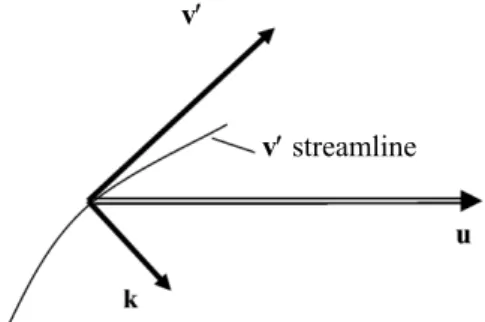
Fig. 1. Representation of the flow field: u, average velocity; v′, velocity fluctuation; k, curvature vector of the velocity fluctuation streamline.
Consider now the dynamical flow characteristic M corresponding to Ω, defined as
, ′
= ×
M v R (5)
where R=k k2
denotes the local curvature radius-vector of the velocity fluctuation streamline. Substitution of the latter relation into Eq. (5) gives
2 2d
, d
R R
t φ ′
= × =
M v k (6)
where R=|R| 1 .= k From Eq. (6) it follows that the quantity M has the meaning of the average angular momentum with R=R2k
in the role of the random moment arm. The defined Ω and M allow us to introduce the effective moment of inertia J as follows:
.
J
=
M Ω (7)
The quantity J determines the characteristic spatial scale of the rotationally anisotropic turbulence constituent contributing to Ω and M. It is easy to see that for the turbulent flows with Ω≠0 the turbulence energy (understood here as the energy of velocity fluctuations)
2 1
2
K= v′ can be naturally decomposed as follows:
0 1
, 2
K= M⋅ +Ω K (8)
where the first term on the right side describes the energy of the rotationally anisotropic part of motion and 0 1
2 ,
K = M′⋅Ω′ where M′=v′×R−M and ,
′=v′× −k
Ω Ω is the residual part of the turbulence energy due to the non-orientated fluctuations. Notice that for the non-vanishing M and/or Ω, the energy described by the first term on the right side of Eq. (8) does not vanish. Therefore, it is natural to expect that systematically anisotropic local rotation characterized by Ω contributes to the dynamical and energetic processes and thus plays a role in forming the average properties of the flow.
The description of turbulent flows with M, Ω≠0 should be based on the conservation laws of average momentum, angular momentum M and energy K0. The component form of the balance equations expressing the first two of these laws can be expressed as
, d
, dtui ij j fi
ρ =σ +ρ (9)
, d
, dtMi mij j eijk jk mi
ρ = − σ +ρ (10)
where i j k, , =1, 2, 3, eijk is the permutation symbol, ρ is (constant) density of the medium (water), σij denotes v′
the components of the stress tensor, fi denotes the
components of the density of body forces per unit mass, mij denotes the components of the
moment-tensor describing the diffusion of M, mi denotes the
components of the density of body moments other than described by the first two terms on the right side of Eq. (10) and the index after the comma denotes differentiation along the respective coordinate and Einstein summation is assumed. In essence, Eq. (9) is the averaged Navier–Stokes (Reynolds) equation (with an asymmetric turbulent stress tensor) and Eq. (10) is the averaged equation obtained via the vector multiplication of the equation for v′ (derived from the Navier–Stokes equation) from the right by R. The technical details of the derivation of Eqs (9) and (10) can be found in Heinloo (2004).
The version of the RAT theory utilized in the current paper particularizes Eqs (9) and (10) by applying the standard closure technique (Heinloo 2004). In particular, the applied closure specifies the vector σ with components
ijk jk
e σ in Eq. (10) as
4 (γ ),
= −ω
σ Ω (11)
in which 1 2 = ∇ ×
ω u is the vorticity and γ is called the
coefficient of rotational viscosity. The coefficient γ in Eq. (11) couples the Ω-field to the vorticity field. Note that this coefficient allows for a more detailed description of the flow properties compared to classical approaches where the viscosity is characterized by the turbulent (eddy) viscosity coefficient. Equation (11) suggests that whenever there is vorticity in the field, it results in generation of nonzero Ω and vice versa.
The model setup
The modification of the classical Ekman model dis-cussed below utilizes Eqs (9) and (10) within the closure introduced in Heinloo (2004). We consider the upper layer of the ocean in the Northern Hemisphere with a constant water density in the right-hand Cartesian coordinate system ( , , ),x y z with the coordinate z
directed downwards and z=0 at the ocean surface. The ocean is forced by the constant wind stress τ= −( τ, 0, 0) directed along the x-axis (τ >0), and
x y
[u ( ),z u ( ), 0].z =
u (12)
For the resulting flow in the coordinate system rotating with the angular velocity, 0
(0, 0, f 2),
= −
ω where f
is the Coriolis parameter, and for the applied closure, Eqs (9) and (10) can be written as follows:
2
0 2
( ) 2 2 0,
z
µ γ+ ∂ + γ∇ × + ρ × =
∂ u Ω u ω (13)
2
2 4( ) 2 0.
J z
ϑ ∂ − γ κ+ + γ∇ × =
∂ Ω Ω u (14)
Equations (13) and (14) differ from the respective equations derived in Heinloo (2004) by the presence of the Coriolis term in Eq. (13). Here (in addition to J and γ explained above) µ is the coefficient of turbulent shear viscosity quantifying the transfer of energy from the average flow to the energy of the non-orientated turbulence constituent 0
,
K κ is the coefficient quantifying the energy transfer from 1
2M⋅Ω to
0
K and ϑ is the coefficient of diffusion of the angular momentum M. It follows from Eqs (13) and (14) that only the horizontal components of Ω are coupled to the flow velocity, therefore, similar to the flow velocity (Eq. (12)), we shall assume that Ω=[Ωx( ),z Ωy( ), 0].z For γ =0 Eq. (13) reduces to the equation of the classical Ekman model and Eq. (14) to an additional equation interpreted as describing the effect of the Stokes drift. In what follows we assume that γ ≠0, consequently, the effect of the Stokes drift is coupled with the motions described by the classical Ekman model.
The solution of Eqs (13) and (14) is assumed to satisfy the following boundary conditions:
lim , 0,
z→∞u Ω= (15)
0
( ) 2 (0) , (0) (0).
z
c z
µ γ γ
=
∂
+ + ⋅ = =
∂
u
Ω τ Ω ω
E (16)
In Eqs (16) E is the Levi-Civita tensor with components ,
ijk
e 1
2
= ∇ ×u
ω is the vorticity and c is a constant, 0< <c 1. The second condition in Eqs (16) simply means that Ω and ω are collinear at the boundary
0.
z= Consequently, the first condition in Eqs (16) can be rewritten as
s 0
, z z µ
=
∂ = −
∂
u
τ (17)
where µs =µ γ+ (1−c)≥µ. All flow-specific coefficients as well as J in Eqs (13) and (14) are treated as constants.
DISCUSSION
Solution for the flow velocity
Defining u!=ux+iuy and Ω Ω= x+iΩy,
! where i is the
2
2
( ) u 2 i i f u 0,
z z
Ω
µ γ+ ∂ + γ ∂ + ρ = ∂
∂
! !
! (18)
2
2 4( ) 2 0,
u
J i
z z
Ω
ϑ ∂ − γ κ Ω+ + γ∂ = ∂ ∂
! !
! (19)
lim , 0, z→∞u Ω =
! ! 0 z s u z τ µ = ∂ = − ∂ ! and 0 (0) . 2 z c u i z Ω = ∂ = ∂ !
! (20)
The solution of Eqs (18)–(20) for u! is expressed as
1( ) 2( ),
u!=u z! +u z!
(21)
where
1 1(0) exp( 1 )
u! =u! λz and
2 2(0) exp( 2 ).
u! =u! λz
(22)
In Eq. (22), λ1 and λ2 are the roots of the biquadratic
equation
4 2
2 2 2 2
1 2
1 1
0,
i i
λ − − λ − =
" " " " (23)
in which ef 2 ( ) 1 1 4 , ( ) J
µ γ κ ϑ µ γ
+ =
+
" 2 2
ef 1 2 1 1 , f f ρ ρ
µ γ µ
= < = +
" " (24)
and 1
ef ( ) .
µ =µ γ κ γ κ+ + −
Only the values of λ1 and
2
λ with negative real parts are compatible with the boundary conditions stated in Eq. (15) and are applied hereafter. The velocity constituents u!1(0) and u!2(0) are
specified as
1 2
1 2 2
s 1 2
exp ( 4)
(0) B i
u τ λ λ π
µ λ λ
− + =
−
! (25)
and
2 1
2 2 2
s 1 2
exp ( 4)
(0) B i ,
u τ λ λ π
µ λ λ
− =
−
! (26)
where 1
s 2( ef ) 0.
B=µ" µ " − >
Equations (21)–(26) represent the vertical dis-tribution of the average flow velocity depending on
1
s ,
τµ− 1
s ef
µ µ −
and on three characteristics of turbulence properties of the medium "<"2<"1 with the dimension
of length.
Properties of the vertical structure of velocity
Consider the solution of Eq. (23) for λ12 and 2 2 λ in the following representation:
2 2
1 1 exp(i )
λ = λ ψ and 2 2
2 2 exp[ (3i 2 )],
λ = λ π −ψ (27)
where 0≤ ≤ψ π 2, 2 2
1 1
|λ | |= λ | and 2 2
2 2
|λ | |= λ | , while 1
1 2 2
|λ λ|| | (= "" )− and
1 2
|λ | |> λ | . Using Eq. (27), we have for λ1 and λ2
1 1 exp(i )
λ = −λ ϕ
and
2 2 exp[ (3i 4 )] 2 exp[ i( 4)],
λ = λ π −ϕ = −λ − ϕ π+
where 0≤ =ϕ ψ 2≤π 4. When denoting the e-folding scales for u!1 and u!2 by
11 1 1 1 1 0 Re cos h
λ λ ϕ
= − = >
and
21
2 2
1 1
0,
Re cos( 4)
h
λ λ ϕ π
= − = >
+
and the respective rotation scales of u!1 and
2
u! by
12 1 1 1 1 0 Im sin h
λ λ ϕ
= − = >
and
22
2 2
1 1
0,
Im sin( 4)
h
λ λ ϕ π
= = >
+
the expressions for u!1 and u!2 in Eq. (22) can also be
rewritten as
1 1
11 12
2 2
21 22
(0) exp exp ,
(0) exp exp .
z z
u u i
h h
z z
u u i
h h = − − = − ! ! ! ! (28)
In the following we interpret the velocity constituents
1
u! and
2
Let us emphasize the following properties of the solution given by Eqs (21) and (28).
1. For γ= c=0 and 12 12
E (2 ) (µ ρf) ,
−
<< =
" " where
E
" is the Ekman depth in its classical sense,
we have 1
1 ,
λ = −"− 1
2 (i 1) E,
λ = − "−
1(0) 0,
u! =
1 2
2(0) ( ) exp ( 4),
u! =τ ρ µf − iπ
21 22 E
h =h =" and the solution given by Eqs (21) and (28) reduces to the classical solution for the Ekman boundary layer
E E
exp exp .
4
z z
u i
f
τ π
ρ µ
= − +
!
" " (29)
2. The integral volume transport in the Ekman layer,
0
,
i udz
f
τ ρ
∞
=
∫
!coincides with the transport following from the classical Ekman’s theory.
3. Due to
1 2
s 1 2
1 exp ( 4)
(0) (0) (0) B i ,
u u u τ π
µ λ λ
+
= + = −
+
! ! !
the angle between the surface wind stress and the surface drift velocity in general differs from π 4 predicted by the classical Ekman solution. In particular, for "<<"E (considered as the most
typical) we have u!(0)≈ −τ µ" s(1+Bexp (iπ 4))
determining the angle between the surface wind stress and surface drift velocity between 0 (the Stokes drift situation) and π 4 (the classical Ekman situation).
4. The e-folding scale of u!2 exceeds the e-folding
scale of u!1 (h21>h11), i.e., the characteristic vertical
extent of the Ekman drift layer is larger than the characteristic vertical extent of the Stokes drift layer. 5. Due to the opposite signs of the arguments of
the exponent −i z h12 and i z h22 in Eq. (28), the
velocity constituents u!1 (the Stokes drift velocity
constituent) and u!2 (the Ekman drift velocity
constituent) rotate with depth in opposite directions. 6. While the e-folding scale of the Ekman drift velocity
constituent u!2 exceeds its rotation depth scale
21 22
(h >h ), the rotation scale of the Stokes drift velocity constituent u!1 exceeds its e-folding scale
11 12
(h <h ).
7. While the scales h21 and h11 both decrease, h22 and
12
h increase for decreasing ϕ (so that for ϕ=0 we have h12=h22). Therefore, the properties of
the Ekman and Stokes layers are in general interdependent.
Although the discussed solution was derived for the Northern Hemisphere, it holds also for the Southern Hemisphere (where the y-axis is reversed to form the left-hand coordinate system ( , , )).x y z
Comparison with the observed data
Properties 1–7 demonstrate that the derived solution is sufficiently flexible to mimic the observed velocity distributions (cited in the Introduction) that diverge from the vertical structure predicted by the classical Ekman solution. In agreement with Cushman-Roisin (1994), the modification includes the situation with the angle between the wind and the surface drift velocity vectors different from π 4. Figure 2 exemplifies this situation on the velocity spiral of the non-dimensional
velocity 1
s( ) u
µ τ" − !
calculated for 1 s ef 0.07, µ µ − =
10 m, = "
1=60 m
" and
2=50 m.
" The surface velocity is veering by 18.3° to the right of the wind direction. On the basis of the observed data it has been stated in several investigations (Weller 1981; Price et al. 1986, 1987; Wijffels et al. 1994; Chereskin 1995; Schudlich & Price 1998; Price & Sundermeyer 1999; Chereskin & Price 2001; Lenn & Chereskin 2009) that the rotation scale of velocity profiles exceeds the
e-folding scale of the velocity norm. The suggested
Fig. 2. Velocity spiral for the modelled non-dimensional velocity µs(τ")
−1ũ, corresponding to µ
sµef−1 = 0.07, " = 10 m,
"1 = 60 m and "2 = 50 m (Vx = µs(τ")
−1
Reũ and Vy = µs(τ")
−1
modified solution includes this effect. As an example, in case of the velocity spiral shown in Fig. 2, the e-folding and the rotation scales of the velocity are 15 and 24 m, respectively.
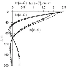
Figure 3 presents the data of the flow velocity relative to the reference level at z=98 m (circles) collected in the Drake Passage (adopted from Lenn & Chereskin 2009) together with the corresponding velocity distributions calculated from Eqs (21) and (28) (solid curves) and the Ekman solution calculated from Eq. (29) (dashed curves). The modelled velocity distribution is calculated for 1
s ef 0.77, µ µ− =
14 m, = "
1=32 m,
"
2=31 m,
" 1 1
s 0.115 s
τµ− = −
and the Ekman velocity distribution for "E=44 m,
1
2 1
( f ) 0.032 m s .
τ ρ µ − = −
It can be seen in Fig. 3 that, firstly, the modified solution fits better the observed data than the Ekman solution. Secondly, the e-folding scale of the Ekman layer ("E) predicted by the Ekman solution exceeds the
characteristic e-folding scale (max{ ,"1 "2}) predicted by the modified solution. Thirdly, the classical Ekman solution matches the observed data in Fig. 3 rather well, therefore the rotation scale of the vertical distribution of velocity is close to its e-folding scale. This conclusion, however, contradicts Lenn & Chereskin (2009), where, based on the same data set, the rotation scale of the vertical distribution of velocity has been estimated to exceed its e-folding scale by 2–3 times. The indicated contradiction follows from a specific feature of Lenn & Chereskin (2009) analysis. Their analysis was applied to
Fig. 3. The depth-dependence of the velocity components Re(ũ – Ũ) and Im(ũ – Ũ), where Ũ is the velocity at the reference level z = 98 m, calculated according to the suggested model for µsµef
−1
= 0.77, " = 14 m, "
1 = 32 m, "2 = 31 m,
τµs
−1
= 0.115 s−1 (solid curves) and according to the Ekman model for "E = 44 m, τ(ρfµ)−½ = 0.032 m s−1 (dashed curves)
compared with data (circles) adopted from Lenn & Chereskin (2009).
the velocity data from which the velocity at the assumed reference level of z=98 m had been subtracted. The resulting velocity equals to zero at the selected reference level. As a consequence, the e-folding scale becomes dependent on the reference level depth and no more characterizes the underlying physical process.
CONCLUSIONS
The Ekman layer studies (Huang 1979; Davis et al. 1981; Weller 1981; Price et al. 1986, 1987; Richman et al. 1987; Weller et al. 1991; Cushman-Roisin 1994; Wijffels et al. 1994; Chereskin 1995; Schudlich & Price 1998; Price & Sundermeyer 1999; Chereskin & Price 2001; Lenn & Chereskin 2009) have shown that the observed vertical distributions of velocity in the ocean Ekman layer often deviate from the distribution predicted by the Ekman theory. The suggested modified Ekman model explains the observed deviations from the point of view of the turbulence mechanics in Heinloo (2004) accounting for the curvature effects of the velocity fluctuation streamlines on the formation of the average flow properties. The curvature effects are accounted for through the average vector product of the velocity fluctuations and the local curvature vectors of their streamlines at all points of the flow field. This approach makes it possible to systematically account for phenomena (such as the Stokes drift or the generation of rotationally anisotropic part of the motion) affecting the structure of the Ekman layer. It is shown that the additional included effects can explain the observed deviations from the Ekman theory and agree with the data measured in the Drake Passage adopted from Lenn & Chereskin (2009).
Acknowledgements. The authors thank the anonymous referee whose critical comments helped to modify the style of the paper and to bring the presentation to the commonly accepted standards.
REFERENCES
Chereskin, T. K. 1995. Direct evidence for an Ekman balance in the California Current. Journal of Geophysical Research, 100, 18261−18269.
Chereskin, T. K. & Price, J. F. 2001. Ekman transport and pumping. In Encyclopedia of Ocean Sciences (Steele, J., Thorpe, S. & Turekian, K., eds), pp. 809−815. Academic Press.
Coleman, G. N., Ferziger, J. H. & Spalart, P. R. 1990. A numerical study of the turbulent Ekman layer. Journal of Fluid Mechanics, 213, 313−348.
Davis, R., deSzoeke, R., Halpern, D. & Niiler, P. 1981. Variability in the upper ocean during MILE. Part 1: The heat and momentum balances. Deep-Sea Research, 28A, 1427−1451.
Ekman, V. W. 1905. On the influence of the Earth’s rotation on ocean currents. Arkiv för Matematik, Astronomi och Fysik, 2, 1−53.
Heinloo, J. 2004. The formulation of turbulence mechanics. Physics Review E, 69, 056317.
Huang, N. E. 1979. On surface drift currents in the ocean. Journal of Fluid Mechanics, 91, 191−208.
Lenn, Y.-D. & Chereskin, T. K. 2009. Observations of Ekman currents in the Southern Ocean. Journal of Physical Oceanography, 39, 768−779.
Madsen, O. S. 1977. A realistic model of the wind-induced Ekman boundary layer. Journal of Physical Oceanography, 7, 248−255.
Phillips, O. M. 1977. Dynamics of the Upper Ocean. Cambridge University Press, 336 pp.
Price, J. F. & Sundermeyer, M. A. 1999. Stratified Ekman layers. Journal of Geophysical Research, 104(C9), 20467−20494.
Price, J. F., Weller, R. A. & Pinkel, R. 1986. Diurnal cycling: observations and models of the upper ocean response to diurnal heating, cooling, and wind mixing. Journal of Geophysical Research, 91, 8411−8427.
Price, J. F., Weller, R. A. & Schudlich, R. R. 1987. Wind-driven ocean currents and Ekman transport. Science, 238, 1534−1538.
Richman, J. G., deSzoeke, R. A. & Davis, R. E. 1987. Measurements of near-surface shear in the ocean. Journal of Geophysical Research, 92, 2851−2858. Schudlich, R. R. & Price, J. F. 1998. Observations of seasonal
variation in the Ekman layer. Journal of Physical Oceanography, 28, 1187−1204.
Weller, R. A. 1981. Observations of the velocity response to wind forcing in the upper ocean. Journal of Geophysical Research, 86, 1969−1977.
Weller, R. A., Rudnick, D. L., Eriksen, C. C., Polzin, K. L., Oakey, N. S., Toole, J. W., Schmitt, R. W. & Pollard, R. T. 1991. Forced ocean response during the Frontal Air–Sea Interaction Experiment. Journal of Geophysical Research, 96, 8611−8638.
Wijffels, S., Firing, E. & Bryden, H. L. 1994. Direct observations of the Ekman balance at 10° N in the Pacific. Journal of Physical Oceanography, 24, 1666−1679.
Zikanov, O., Slinn, D. N. & Dhanak, M. R. 2003. Large-eddy simulations of the wind-induced turbulent Ekman layer. Journal of Fluid Mechanics, 495, 343−368.