Minimizing makespan of a resource-constrained scheduling problem: A hybrid greedy and genetic algorithms

(1)

International Journal of Industrial Engineering Computations 6 (2015) 503–520

Contents lists available at GrowingScience

International Journal of Industrial Engineering Computations

homepage: www.GrowingScience.com/ijiec

Minimizing makespan of a resource-constrained scheduling problem: A hybrid

greedy and genetic algorithms

Aidin Delgoshaei*_{, Mohd Khairol Mohd Ariffin, B. T. Hang Tuah Bin Baharudin and Zulkiflle Leman}

University Putra Malaysia, Department of Mechanical and Manufacturing Engineering, Faculty of Engineering, 43400 UPM, Serdang, Kuala Lumpur, Malaysia

C H R O N I C L E A B S T R A C T

Article history:

Received January 16 2015 Received in Revised Format April 10 2015

Accepted May 10 2015 Available online May 14 2015

Resource-Constrained Project Scheduling Problem (RCPSP) is considered as an important project scheduling problem. However, increasing dimensions of a project, whether in number of activities or resource availability, cause unused resources through the planning horizon. Such phenomena may increase makespan of a project and also decline resource-usage efficiency. To solve this problem, many methods have been proposed before. In this article, an effective backward-forward search method (BFSM) is proposed using Greedy algorithm that is employed as a part of a hybrid with a two-stage genetic algorithm (BFSM-GA). The proposed method is explained using some related examples from literature and the results are then compared with a forward serial programming method. In addition, the performance of the proposed method is measured using a mathematical metric. Our findings show that the proposed approach can provide schedules with good quality for both small and large scale problems.

Keywords: Project Scheduling Resource-constrained Backward Approach Makespan Genetic Algorithm

1. Introduction

Classic Resource-constrained project scheduling problem, which is dealt with scheduling the project activities considering time and resource constraints, is generalized for minimizing completion time of the project (makespan) (Kelley, 1963). Normally, In RCPSP, activities are scheduled by considering two types of constraints:

I) The executive priority relations between activities which are expressed by relation matrix II) The availability resources level for executing activities

As a consequence, final solution must be feasible in both priority and resource level. During the last few decades, several researches have addressed the RCPSP models by considering varied objectives, constraints and solution solvers using either optimizing or heuristic approaches (Demeulemeester, 2002; Kolisch & Hartmann, 1999). In this manner, a peer review on RCPSP models, objective functions, constraints and limitations and some approaches was prepared by Hartmann and Briskorn (2010). They

* Corresponding author.

(2)

mostly focused on objectives such as minimizing�_��, minimal and maximal time lags and net present value (NPV).

Traditionally, classical RCPSP models are developed for minimizing �_��(Patterson et al., 1989; Talbot, 1982). But, during the last 2 decades, scientists have developed more RCPSP problems considering varied objectives. Mainly, authors tackle RCPSP with four optimization criteria: 1)�_�� minimization, where an attempt has been accomplished to minimize the total elapsed time among time horizon of the project. 2) NPV maximization has been developed to maximize profit of the project while positive and/or negative cash flows were taken into consideration (RCPSP-CF) (Delgoshaei et al., 2014; Seifi & Tavakkoli-Moghaddam, 2008; Sung & Lim, 1994; Ulusoy et al., 2001; Yang et al., 1993) .3) Cost minimization where declining of total cost of the project is the main objective of the problem (Laslo, 2010). 4) Optimizing robustness of solutions. For this purpose a trade-off between quality-robustness and solution-robustness in RCPSP has been accomplished while safety times (spread time buffers throughout the project time horizon) in project scheduling were taken into consideration (Van de Vonder et al., 2005). Afterward, a similar research was accomplished focusing on resource constraint impacts (Van de Vonder et al., 2006). RCSPs can be developed using single objective function or multi –objective functions. In this manner, a time dependent cost structure for minimizing completion time by using extra resources which cause faster execution of activities was developed by Achuthan and Hardjawidjaja (2001). Afterward, 2 more versions of resource-constraint multi project scheduling problem were developed in a way that in first version, the activity durations are considered fixed but in second one, a project duration function is used to decrease the amount of resource allocating (Lee & Lei, 2001). Effects of the serial and parallel scheduling schemes while using multi- and single-project approaches were analysed later (Lova & Tormos, 2001). It was found that using parallel scheduling schemes and multi-project approach could provide a basis for managers to minimize mean multi-project delay or multi-multi-project duration increasing. Hence, Kim et al. (2005) proposed a hybrid of GA with fuzzy logic controller (FLC-HGA) to solve the resource-constrained multiple project scheduling problem (RC-MPSP). The proposed approach worked based on using genetic operators with fuzzy logic controller (FLC) through initializing the revised serial method with precedence and resources constraints. Afterward, an attempt has been accomplished for minimizing�_��, as well as maximizing solution robustness by increasing float time maximization (Abbasi et al., 2006). In another study, a two-stage algorithm was developed for RCPSP while minimize�_��, considered as an acceptance threshold for the second stage and then, in next stage, a set of 12 alternative robust predictive indicators was employed to maximize robustness of the project (Chtourou & Haouari, 2008). Ke and Liu (2010) focused on project scheduling problem while fuzzy activity duration times were taken into consideration. They used fuzzy concepts for minimizing�_�� in an integrated fuzzy-based GA.

(3)

In this article, a new method for rescheduling RCPSP to improve�_��, using unused resources where all resources were considered pre-emptive is executed. For this purpose, we developed a backward method by employing a hybrid greedy search and GA, which was formulated as a non-linear mixed integer programming (NL-MIP) model.

2. Materials and Methods

The mathematical model, proposed in this paper, is developed in a way that activities can be split through planning horizon where time horizon is divided to � slots to be proper for tracking the rescheduling process. It should be emphasized that, the proposed model is developed as single activity mode to make investigating of the proposed method easier.

The assumptions of the model are defined as follow:

1. Model is presented in AON (Activity on Node) structure. 2. Resources are renewable.

3. The renewable resources have limited capacities.

4. Activities are allowed to move only in their free float time. 5. Activity splitting is allowed.

6. All movements have been considered in both backward and forward modes respecting to the precedence relations.

7. Initial scheduling of activities will be performed using forward serial programming. 8. Rescheduling over �_�� is prohibited.

Input arguments and variables for the proposed model are defined as:

Inputs

� ∈ ��

� ∈[1, … ,�] ��

Parameters

�� Maximum amount of resource type k

��,� Required amount of resource r for performing activity i in each time slot �� Executive duration of activity i

�� Time horizon

�� Precedence vector for activity i

Binary Variables

��,��

1 if activity � executed in time slot �

0 ��ℎ��

Integer Variables

��: Start time of activity i Mathematical Model

The proposed model in this research is a pertinent version of Peteghem and Vanhoucke (2010) where greedy selection of activities for using unscheduled resources is taken into consideration.

��: � � �.�_�,� ��

�=1 �

�=1

(1)

subject to

(4)

��≥ ��,�.��=1�ℎ��.��,��; ∀�,� ∈ � (3)

� � ��,� �

�=1 .�_�,� ��

�=1

≤ �� ; ∀� ∈ �

(4)

��,�.��≤ �; ∀� ∈ � ,� ∈ �� (5)

��,�.��=��; ∀� ∈ � ,� ∈ �� (6)

��: �� (7)

��,�: �� (8)

For the proposed model, minimization of �_��by considering renewable resources is considered as the main objective. Using � as a part of objective function (�_�_,_�.�) helps model use backward movements for minimizing �_�� as early scheduling of activities causes lower amounts for t and consequently lower value for the objective function.

First constraint in this model is defined as determination of initial start of each activity, which helps model start from a feasible solution. Second constraint ensures the feasibility of the activities precedence relations. Using the term ��_�=1�ℎ ��.�_�,�� helps activities start not earlier than their predecessors last

execution day. It is important to know that using standard definition of early start of activities (��_� =

��+�� ℎ�� ∈ ��) is not suitable for applying for allowed activity splitting RCPSPs and may cause

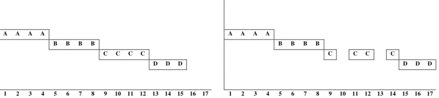
wrong results. To explain more, suppose it is decided to calculate the early start of activity � in 2 modes where in the first mode the activity splitting is forbidden while in the second mode it is allowed (Fig. 1).

A A A A A A A A

B B B B B B B B

C C C C C C C C

D D D D D D

1 2 3 4 5 6 7 8 9 10 11 12 13 14 15 16 17 1 2 3 4 5 6 7 8 9 10 11 12 13 14 15 16 17

Fig. 1. Comparing Different Styles of Calculating ES with and without Activity Splitting (Left to Right)

In the left Gantt of Fig. 1, while splitting is not allowed, ��_�will be calculated correctly by using the standard formula (��_� = ��_�+�_�). But, as seen, calculating early start of activity D while activity splitting is allowed (right figure) will not be 13 das anymore since activity C is split two times in days 10 and 13 and therefore it cannot be finished earlier than day 14. Consequently, activity D cannot be started sooner than the day 15. Therefore, to prevent such error, the above formula is modified for calculating ES of each activity considering the real planning dates, Eq. (9):

�� ≥ ��=1�ℎ ��,�.��; ∀ (�,�) ∈ � (9)

(5)

3. The Proposed Method

Genetic algorithms (GA) are iterative search procedures that work based on the biological process of natural selection and genetic inheritance, which maintain a population of a number of candidate members over many simulated generations. Hopefully, good characteristics of the population members that will be retained over the generations can maximize a pre-determined fitness function.

In general, the main steps of the proposed greedy-based GA procedure are (Fig. 2):

Step 1) Create an initial population,

Step 2) Use selecting operator to update tournament list, Step 3) Run greedy algorithm as crossover operator of GA:

• Run Selecting operator (Crossover)

• Run Feasibility check operator

• Run Solution check operator

Step 4) Calculate mutation probability function, Step 5) Run mutation operator (if needed),

Step 6) Terminate the searching process if stopping criteria are met, otherwise go to Step 2.

Fig. 2. Structure of the Proposed GA-based Method

3.1 Population Size

Generally metaheuristic algorithms quickly respond to small size or relaxed resource RCPSPs but while large scale problems are taken into account choosing appropriate population size for such algorithms plays essential rule to solve experiments. For this purpose a GA coding operator is developed which suggests the suitable, but not necessarily the best, population size according to the equation below:

��(��_�)

�� ;∀ � (10)

Eq. (10) consists on the largest frequency of the resource demands. The genetic algorithm maintains a collection (population) of solutions in each generation until the end of the searching process.

3.2 String Representation

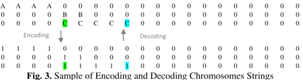
The proposed GA requires a unique solution string representation scheme. In this study, authors applied binary representative scheme which seems appropriate to present strings of solutions. The encoding of solutions in the proposed procedure is ‘one-to-one’, which refers to solutions that are represented by � (activity number) binary strings as chromosomes. Chromosomes contain sets of � genes where each gene is a binary digit in its nature:

��(_�,�,�,�,�) = �

1; if activity � performs in date � 0; else

(11)

Start

Generate Initial Population

Feasible Solution N

Selecting Operator G=1

G=G+1

Y

Cross over Operator

Feasible Solutions

Mutation Operator

Mutation

Stopping Criteria

Finish Y

Y N

Pass

Reject

(6)

where� demonstrates population size and � presents generation. Fig. 3 shows an example of encoding and decoding chromosome strings:

A A A A 0 0 0 0 0 0 0 0 0 0 0 0 0 0 0 0

0 0 0 0 B B 0 0 0 0 0 0 0 0 0 0 0 0 0 0

0 0 0 0 C C C C C 0 0 0 0 0 0 0 0 0 0 0

1 1 1 1 0 0 0 0 0 0 0 0 0 0 0 0 0 0 0 0

0 0 0 0 1 1 0 0 0 0 0 0 0 0 0 0 0 0 0 0

0 0 0 0 1 1 1 1 1 0 0 0 0 0 0 0 0 0 0 0

Fig. 3. Sample of Encoding and Decoding Chromosomes Strings

3.3 Initial Solution Generator

During the first stage, the proposed approach provides � (pop-size) initial time networks which are both precedence- and resource-feasible but are scheduled in maximum time horizon that is defined as upper bound (��_�_,_�) for the problem. Note that each solution in this stage contains a set of chromosomes that meet priority requirements:

��,� = ∑��=1max �� (�)�� (12)

Using upper bound strategy in this step will guarantee precedence- and resource-feasibility for initial solutions and at the same time it can be considered as a good threshold for measuring efficiency of the solutions in final stage.

��_��_�� (: , : ,�,�)

A ₁ ₁ ₁ ₁ ₀ ₀ ₀ ₀ ₀ ₀ ₀ ₀ ₀ ₀ ₀ ₀ ₀ ₀ ₀ ₀ ₀ ₀ ₀ ₀ ₀ ₀ ₀ ₀ ₀ ₀ ₀ ₀

B ₀ ₀ ₀ ₀ ₀ ₀ ₀ ₀ ₀ ₀ ₀ ₀ ₀ ₀ ₀ ₀ ₁ ₁ ₀ ₀ ₀ ₀ ₀ ₀ ₀ ₀ ₀ ₀ ₀ ₀ ₀ ₀

C ₀ ₀ ₀ ₀ ₀ ₀ ₀ ₀ ₁ ₁ ₁ ₁ ₁ ₀ ₀ ₀ ₀ ₀ ₀ ₀ ₀ ₀ ₀ ₀ ₀ ₀ ₀ ₀ ₀ ₀ ₀ ₀

D ₀ ₀ ₀ ₀ ₁ ₁ ₁ ₁ ₀ ₀ ₀ ₀ ₀ ₀ ₀ ₀ ₀ ₀ ₀ ₀ ₀ ₀ ₀ ₀ ₀ ₀ ₀ ₀ ₀ ₀ ₀ ₀

E 0 0 0 0 0 0 0 0 0 0 0 0 0 0 0 0 0 0 0 0 0 1 1 1 0 0 0 0 0 0 0 0

F 0 0 0 0 0 0 0 0 0 0 0 0 0 0 0 0 0 0 0 0 0 0 0 0 1 1 1 1 0 0 0 0

G ₀ ₀ ₀ ₀ ₀ ₀ ₀ ₀ ₀ ₀ ₀ ₀ ₀ ₁ ₁ ₁ ₀ ₀ ₀ ₀ ₀ ₀ ₀ ₀ ₀ ₀ ₀ ₀ ₀ ₀ ₀ ₀

H ₀ ₀ ₀ ₀ ₀ ₀ ₀ ₀ ₀ ₀ ₀ ₀ ₀ ₀ ₀ ₀ ₀ ₀ ₀ ₀ ₀ ₀ ₀ ₀ ₀ ₀ ₀ ₀ ₁ ₁ ₀ ₀

I ₀ ₀ ₀ ₀ ₀ ₀ ₀ ₀ ₀ ₀ ₀ ₀ ₀ ₀ ₀ ₀ ₀ ₀ ₁ ₁ ₁ ₀ ₀ ₀ ₀ ₀ ₀ ₀ ₀ ₀ ₀ ₀

J 0 0 0 0 0 0 0 0 0 0 0 0 0 0 0 0 0 0 0 0 0 0 0 0 0 0 0 0 0 0 1 1

��_��_�� (: , : ,�,�)

A ₁ ₁ ₁ ₁ ₀ ₀ ₀ ₀ ₀ ₀ ₀ ₀ ₀ ₀ ₀ ₀ ₀ ₀ ₀ ₀ ₀ ₀ ₀ ₀ ₀ ₀ ₀ ₀ ₀ ₀ ₀ ₀

B ₀ ₀ ₀ ₀ ₀ ₀ ₀ ₀ ₀ ₀ ₀ ₀ ₀ ₁ ₁ ₀ ₀ ₀ ₀ ₀ ₀ ₀ ₀ ₀ ₀ ₀ ₀ ₀ ₀ ₀ ₀ ₀

C ₀ ₀ ₀ ₀ ₀ ₀ ₀ ₀ ₁ ₁ ₁ ₁ ₁ ₀ ₀ ₀ ₀ ₀ ₀ ₀ ₀ ₀ ₀ ₀ ₀ ₀ ₀ ₀ ₀ ₀ ₀ ₀

D 0 0 0 0 1 1 1 1 0 0 0 0 0 0 0 0 0 0 0 0 0 0 0 0 0 0 0 0 0 0 0 0

E 0 0 0 0 0 0 0 0 0 0 0 0 0 0 0 0 0 0 0 0 0 0 1 1 1 0 0 0 0 0 0 0

F ₀ ₀ ₀ ₀ ₀ ₀ ₀ ₀ ₀ ₀ ₀ ₀ ₀ ₀ ₀ ₀ ₀ ₀ ₁ ₁ ₁ ₁ ₀ ₀ ₀ ₀ ₀ ₀ ₀ ₀ ₀ ₀

G ₀ ₀ ₀ ₀ ₀ ₀ ₀ ₀ ₀ ₀ ₀ ₀ ₀ ₀ ₀ ₁ ₁ ₁ ₀ ₀ ₀ ₀ ₀ ₀ ₀ ₀ ₀ ₀ ₀ ₀ ₀ ₀

H ₀ ₀ ₀ ₀ ₀ ₀ ₀ ₀ ₀ ₀ ₀ ₀ ₀ ₀ ₀ ₀ ₀ ₀ ₀ ₀ ₀ ₀ ₀ ₀ ₀ ₁ ₁ ₀ ₀ ₀ ₀ ₀

I 0 0 0 0 0 0 0 0 0 0 0 0 0 0 0 0 0 0 0 0 0 0 0 0 0 0 0 1 1 1 0 0

J 0 0 0 0 0 0 0 0 0 0 0 0 0 0 0 0 0 0 0 0 0 0 0 0 0 0 0 0 0 0 1 1

Fig. 4. Samples of Using Upper-bound in Forward Serial Programming

Fig. 4 that is retrieved from optimizing process of an experiment, shows two members in a generation for an example contains 10 activities. It can be seen, activities are scheduled in a serial mode among time horizon without time overlapping. This will avoid resource over allocating in time networks that will remain through optimization process.

Tournament List and Fitness Function

The selection operator is defined to select parents from the population in generations. Individual's selection procedure operates as follows:

• Time-based selecting operator which is developed to select those activities that have positive free slack after scheduling by forward serial programming in first stage. Such activities can move backward or forward respecting to the precedence matrix and without affecting the critical path(s).

a) Suppose activity X has been scheduled to start at ES_t. � ∈ �_� are the defined as predecessors of activity X.

b) FS_X = min �∈��(LFi).

c) If FS_X > 0 then Tournamet. list_i = X.

(7)

Note that population size operator will select individuals in the way that population size remained fixed through the optimizing process.

3.4. Crossover Operator

The main genetic operator is the crossover, which has the role of combining pieces of information from different individuals in the population. In this article, crossover operator will perform as a greedy algorithm. To explain crossover operator, we must first explain Precedence Constraint Posting (PCP) that is considered as an effective strategy for minimizing �_�� (Lombardi & Milano, 2012; Policella et al., 2007). In PCP, sets of initial precedence constraints or precedence operators are amplified through solving process to prevent resource over-allocating. In this research we used greedy algorithm for creating PCP (

Table 1). Normally, greedy algorithms must have at least (but not last) the following 3 steps: selecting operator, feasibility check and solution check.

I) Selecting operator (backward movement): when an activity is selected randomly for crossing over, the first step is to find maximum available backward movement which is a maximum of��_�_{∈��}_�. As a result, procedure finds the maximum possible time slots for backward movements called ��_�. Activity slots are scheduled for backward movements for ��_� members from minimum member sequentially.

II) Feasibility Check: the resource availability operator is employed to check the availability of slot backward movement using the equation:

∑�−1�=1��,� ≤ �� − ��,� �� ∈ �� (13)

III) Selecting operator (forward movement): the function of this operator is avoiding resource confliction among activities during a backward move where such transferring causes resource over-allocation. For this manner, if the resource availability constraint does not satisfy for each member of ��_� then PCP operator will find the nearest forward neighbor (time slot) to set the activity.

Solution Check: in this step the value of the solution will be checked using fitness function. In this research we considered �_�� as fitness function that can be calculated as sum of time slots of activity execution of all activities:

� � ��,�.

�

�=1 ��

�=1 �

(14)

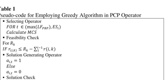
Table 1

Pseudo-code for Employing Greedy Algorithm in PCP Operator

 Selecting Operator

�� ∈(max (��_��),��_�)

��

 Feasibility Check For�_�

��(�,�)≤ ��− ∑ �1�−1 (�,�)

 Solution Generating Operator ��,�= 1

�� ,�= 0  Solution Check

(8)

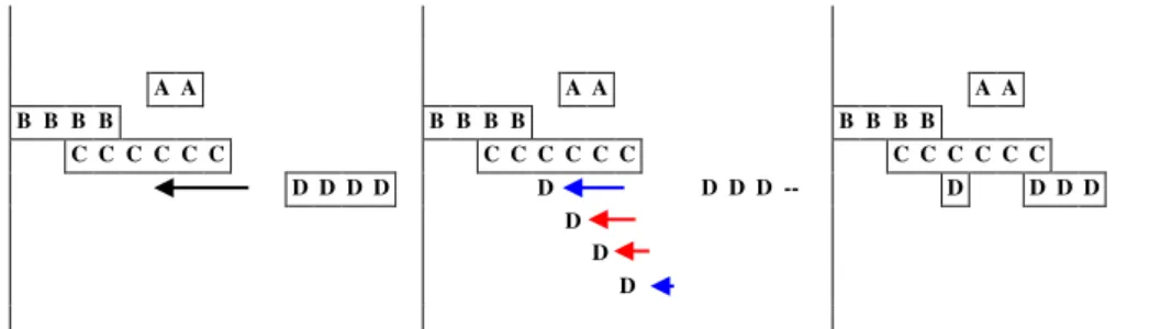
defined as a predecessor of activity�. The resource availability for backward movement (see black arrow in left Gantt of figure 5) is enough to let activity � being started at (��_�+ 1)∈��_�, but for the next two coming days since the all resource capacity is filled by activity �, the backward operator will not let activity � to continue until activity � is finished (see Fig. 5, the middle Gantt). Hence, forward Operator seeks for the first possible time to schedule activity � which is��_�+ 1. This phenomena causes a split in activity � (see Fig. 5, the right Gantt) but will demonstrate using remain resource among ��_� which will cause increasing usage of remained resource during planning horizon.

A A A A A A

B B B B B B B B B B B B

C C C C C C C C C C C C C C C C C C

D D D D D D D D -- D D D D

D D

D

Fig. 5. Opportunity for Backward Movement (Left Gantt); Activity D is Not Allowed Shift Back to LF(B)+2 (Middle Gantt); Activity “D” Rescheduled to LF(A)+1 instead (Right Gantt)

3.5 Mutation Operator

The mutation operator is used to rearrange the structure of a chromosome which possibly is helpful for escaping from local optimum or crowding phenomena. In this article, a single bit string mutation is used to rearrange the position of two gens in a chromosome and to swap their contents. The probability function of mutation operator is formulated as below:

�� =�� , ��

(�)

max (��(�₁),��(�₂))� (15)

where �_��(�) is the total makespan for a new chromosome and �_��(�₁) & �_��(�₂) are the achieved makespan for parents and � is a parameter between 0 and 1.

This equation prevents GA to leave a certain solution space area even if the hybrid algorithm cannot find good solutions inside the area. Consequently, if crossover operator does not improve the new born chromosome the chance of using mutation operator will increase. Such typical function can help us pass local optimum traps. The developed mutation operator, replaces the ��ℎ gene in the string (Fig. 6):

A A A A A A A A A

B B B B B B B B B

C C C C C C C C C

D D D D D D D D D

E E E E E E E E E

1 2 3 4 5 6 7 8 9 10 11 12 13 14 15 16 17 1 2 3 4 5 6 7 8 9 10 11 12 13 14 15 16 17 1 2 3 4 5 6 7 8 9 10 11 12 13 14 15 16 17

Solution 1 Solution 2 Solution 1 (After Mutation)

Fig. 6. A typical Bit string Mutation Operator

(9)

3.6 Stop Criteria

The searching process will be terminated if at least one of these conditions happens:

I) The maximum number of generations is reached.

II) Activities are scheduled in a way that there are no further opportunity for using remain resources during time horizon which means no improvements are possible.

It is important to consider the steady condition of the designed algorithm while solving experiments. For example, if two activities, which are scheduled simultaneously and over allocated through their scheduled period, are bounded by a common successor, the program would never meet a steady condition since it got stock into a loop:

|ES(A)−ES(B)| < |�(�)− �(�)| (16)

Fig. 7. A Graphical Sample of Unsteady Condition of RCSP

Fig. 7 shows that under mentioned condition, activity A and B will be over-allocated during the scheduling process. This means that RCSP system will fall into an unsteady state but it will not pass it. The performance of the proposed hybrid is shown in Table 2.

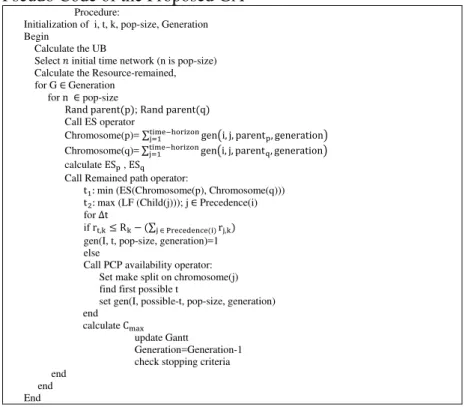
Table 2

Pseudo Code of the Proposed GA Procedure:

Initialization of i, t, k, pop-size, Generation Begin

Calculate the UB

Select � initial time network (n is pop-size) Calculate the Resource-remained, for G ∈Generation

for n ∈ pop-size

Rand parent(p); Rand parent(q)

Call ES operator

Chromosome(p)= ∑time−horizon_j=1 gen�i, j, parentp, generation�

Chromosome(q)=∑time−horizongen�i, j, parentq, generation�

j=1 calculate ES_p , ES_q

Call Remained path operator:

t1: min (ES(Chromosome(p), Chromosome(q)))

t₂: max (LF (Child(j))); j∈ Precedence(i) for ∆t

if rt,k≤Rk−(∑j∈Precedence(i)rj,k)

gen(I, t, pop-size, generation)=1 else

Call PCP availability operator: Set make split on chromosome(j) find first possible t

set gen(I, possible-t, pop-size, generation) end

calculate Cmax update Gantt

Generation=Generation-1 check stopping criteria end

end End

Time

B

A.

St Resource

Resource

ES (A) ES (B) LF (A) LF (B)

(10)

3.7. Using Taguchi method for estimating input parameters

In this research a Taguchi method is used using Minitab®17 in order to survey impacts of input parameters of the proposed hybrid method on completion time of the developed model and also estimate appropriate values for setting the input parameters. For this purpose a �₉ (3^4) orthogonal optimization design is employed (Fig. 8). Table 3 shows the factors and their level in use for the proposed hybrid method.

Table 3

The factors and the levels considering for Taguchi method

Factor Level 1 Level 2 Level 3

A)Number of Generations 5 10 15

B) Pop-size 3 6 9

C) Mutation Rate 0.1 0.2 0.3

Results for: Worksheet 1

Taguchi Design

Taguchi Orthogonal Array Design L9 (3^3)

Factors: 3 Runs: 9

Columns of L9(3^4) Array 1 2 3

Fig. 8. Specifications of the used Taguchi method

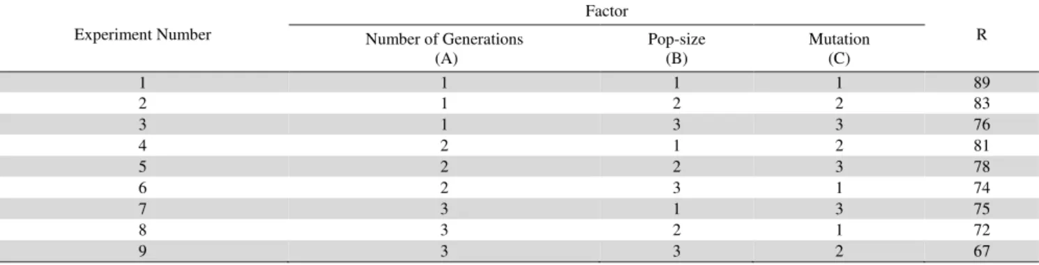
Table 4 shows the experiments designed by Taguchi method. The value R shows the minimum �_�� observed while using the suggested parameters.

Table 4

Results of implemeting the experiments for Taguchi method

Experiment Number

Factor

R Number of Generations

(A)

Pop-size (B)

Mutation (C)

1 1 1 1 89

2 1 2 2 83

3 1 3 3 76

4 2 1 2 81

5 2 2 3 78

6 2 3 1 74

7 3 1 3 75

8 3 2 1 72

9 3 3 2 67

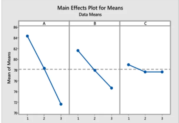
Fig. 9 provides details of analyzing the results of the experiments. As seen, all factors A (the number of generations), B (population size) and C (mutation rate) can improve �_��but with different severity levels. The normal plot of effects that is drawn in Fig. 10 indicates that all factors (the number of generations, population size and mutation rate) have significant impact on the quality of the solutions in the proposed GA but with different values.

Taguchi Analysis: R versus A, B, C Response Table for Signal to Noise Ratios

Smaller is better

Level A B C 1 -38.33 -38.22 -37.64 2 -37.80 -37.79 -37.69 3 -37.06 -37.17 -37.65 Delta 1.27 1.05 0.19 Rank 1 2 3

Response Table for Means

Level A B C 1 82.67 81.67 78.33 2 77.67 77.67 77.00 3 71.33 72.33 76.33 Delta 11.33 9.33 2.00 Rank 1 2 3

Response Table for Standard Deviations

(11)

The downward trend line of factor � in Fig. 11 has a steep slope which reveals the number of generations has the maximum impact while minimizing the�_��. Similarly, number of populations can influence on minimizing �_�� but with less severity. Since the mutation operator has been used rarely, it is obvious that its effects are less than what observed for the other investigated factors. After implementing the method, the regression equation in uncoded Units based on actual values can be determined as:

R = 77.63 - 7.125 A - 2.625 B - 0.8750 C - 0.2070 A×B - 0.1250 A×C - 0.1250 B×C - 0.1250 A×B×C (17)

Fig. 10. The normal plot of the effects between input parameters for the proposed hybrid method

Fig. 11. The main effects plot for showing the impact of levels of input parameters

As seen, in this equation, the interactions between factors can effect on the Y (the expected �_��based on actual values) in a constructive manner. Therefore, for the larger scale experiments the number of generations and the number of population must set maximum and for medium scale problems the focus is on increasing the generation numbers where possible. The mutation rate is considered 0.1 constant for small and medium size problems and for the large scale problems it is considered 0.3.

4. Discussion and Result

To examine and verify robustness of the proposed backward-forward method in improving �_�� in limited time projects while all resources are considered limited and renewable, several problems in small, medium and large sizes are solved by the Matlab® R2009a software on an Intel® Core i7 laptop which is supported by 4 Mb RAM. The Upper bound is considered as time horizon of each problem. To examine the proposed approach, 7 series of numerical examples are designed and solved with 6, 10, 15, 18, 20, 30 and 50 variables. For evaluating the efficiency of proposed model each example is solved under two conditions where all the criteria are considered the same but resource availability. The results, then, checked with results of forward serial programming method (Table 5 and Table 6). At first stage, the initial solutions that are results of using initial solution engine are shown in navy blue time networks. In

Fig. 12.Results of Serial programming, BFSM-GA (Active RCPSP) and BFSM-GA (Relaxed RCPSP)

for Example 11 with 30 variables (Left to Right)

0 -2 -4 -6 -8 -10 -12 -14 -16 99 95 90 80 70 60 50 40 30 20 10 5 1 A A B B C C Factor Name Effect P e rc e n t Not Significant Significant Effect Type C B A

Normal Plot of the Effects (response is R, α = 0.05)

Lenth’s PSE = 0.375 1 2 3

86 84 82 80 78 76 74 72 70 3 2

1 1 2 3

A M e a n o f M e a n s B C

Main Effects Plot for Means Data Means

Activity

(12)

Fig. 13.Results of Serial Programming, BFSM-GA (Active RCPSP) and BFSM-GA (Relaxed RCPSP) for Example 13 with 50 Variables (Left to Right)

Fig. 12 and Fig. 13, results of solving some experimental problems are provided considering 3 status considering results of serial programming, (left Gantts), rescheduling while resource constraints are considered and activity splitting is allowed (middle Gantts) and rescheduling while resource constraints are relaxed (right Gantts). As seen, the proposed approach can effectively reschedule problem to find minimum�_��. But, in second runs, where problems are considered in a way that one or more resources are limited, show how the proposed approach can effectively use remained resources by backward and forward movements which cause activity splitting whenever is needed.

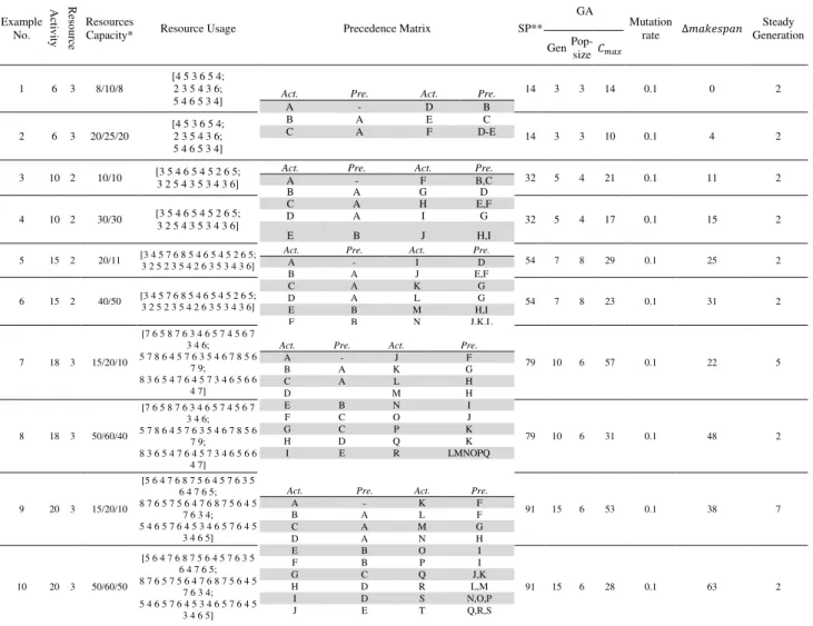
Table 5

Numerical Examples for the Proposed Backward-forward Method

Example No. A ct iv ity R es o u rc e Resources

Capacity* Resource Usage Precedence Matrix SP**

GA

Mutation

rate ∆�� Steady Generation Gen

Pop-size ��

1 6 3 8/10/8

[4 5 3 6 5 4; 2 3 5 4 3 6;

5 4 6 5 3 4] Act. _A Pre. _- Act. _D Pre. _B

B A E C

C A F D-E

14 3 3 14 0.1 0 2

2 6 3 20/25/20

[4 5 3 6 5 4; 2 3 5 4 3 6; 5 4 6 5 3 4]

14 3 3 10 0.1 4 2

3 10 2 10/10 [3 5 4 6 5 4 5 2 6 5; 3 2 5 4 3 5 3 4 3 6]

Act. Pre. Act. Pre.

A - F B,C

B A G D

C A H E,F

D A I G

E B J H,I

32 5 4 21 0.1 11 2

4 10 2 30/30 [3 5 4 6 5 4 5 2 6 5; _{3 2 5 4 3 5 3 4 3 6]} 32 5 4 17 0.1 15 2

5 15 2 20/11 [3 4 5 7 6 8 5 4 6 5 4 5 2 6 5; 3 2 5 2 3 5 4 2 6 3 5 3 4 3 6]

A - I D

B A J E,F

C A K G

D A L G

E B M H,I

F B N J,K,L

G C O M,N

H D

54 7 8 29 0.1 25 2

6 15 2 40/50 [3 4 5 7 6 8 5 4 6 5 4 5 2 6 5;

3 2 5 2 3 5 4 2 6 3 5 3 4 3 6] 54 7 8 23 0.1 31 2

7 18 3 15/20/10

[7 6 5 8 7 6 3 4 6 5 7 4 5 6 7 3 4 6; 5 7 8 6 4 5 7 6 3 5 4 6 7 8 5 6

7 9; 8 3 6 5 4 7 6 4 5 7 3 4 6 5 6 6

4 7]

A - J F

B A K G

C A L H

D M H

E B N I

F C O J

G C P K

H D Q K

I E R LMNOPQ

79 10 6 57 0.1 22 5

8 18 3 50/60/40

[7 6 5 8 7 6 3 4 6 5 7 4 5 6 7 3 4 6; 5 7 8 6 4 5 7 6 3 5 4 6 7 8 5 6

7 9; 8 3 6 5 4 7 6 4 5 7 3 4 6 5 6 6

4 7]

79 10 6 31 0.1 48 2

9 20 3 15/20/10

[5 6 4 7 6 8 7 5 6 4 5 7 6 3 5 6 4 7 6 5; 8 7 6 5 7 5 6 4 7 6 8 7 5 6 4 5

7 6 3 4; 5 4 6 5 7 6 4 5 3 4 6 5 7 6 4 5

3 4 6 5]

A - K F

B A L F

C A M G

D A N H

E B O I

F B P I

G C Q J,K

H D R L,M

I D S N,O,P

J E T Q,R,S

91 15 6 53 0.1 38 7

10 20 3 50/60/50

[5 6 4 7 6 8 7 5 6 4 5 7 6 3 5 6 4 7 6 5; 8 7 6 5 7 5 6 4 7 6 8 7 5 6 4 5

7 6 3 4; 5 4 6 5 7 6 4 5 3 4 6 5 7 6 4 5

3 4 6 5]

91 15 6 28 0.1 63 2

Sp: Steady point (iteration) Act.: Activity Pre.: Predecessor

Activity

(13)

This procedure can decline makespan. Although the approach rearranges activities in order to maximum the usage of remained resources while minimizing �_�� but it is obvious that �_�� can experience its lowest value while resource constraints are relaxed (right Gantts).

Table 6

Numerical Examples for the Proposed Backward-forward Method (Continued from table 5)

No. A ct iv ity R es o u rc e Resources

Capacity* Resource Usage Precedence Matrix SP**

GA

Mutation

rate ∆��

Steady Generation Gen

Pop-size ��

11 30 2 20/25

[5 6 4 7 6 8 7 5 6 4 5 7 6 3 4 6 5 4 7 6 5 6 7 8 5 6 4 7 6 5; 8 7 6 5 7 6 4 5 6 3 4 6 5 4 7 5 6 4 7 6 8 7

5 6 4 5 7 6 3 4]

Act. Pre. Act. Pre. Act. Pre.

A - K E U L-M

B A L F V O

C A M F W P

D A N G X Q-R

E A O H Y ST

F B P H Z N-U

G B Q I AA V-W

H C R J AB X-Y

I D S J AC Z-AA

D T K AD AB-AC

144 15 6 55 0.3 89 9

12 30 2 80/70

[5 6 4 7 6 8 7 5 6 4 5 7 6 3 4 6 5 4 7 6 5 6 7 8 5 6 4 7 6 5; 8 7 6 5 7 6 4 5 6 3 4 6 5 4 7 5 6 4 7 6 8 7

5 6 4 5 7 6 3 4]

144 15 6 36 0.3 108 2

13 50 5 20/30/20

/30/40

[7 6 5 8 7 6 3 4 6 5 7 4 5 6 7 3 4 6 5 7 8 6 4 5 7 6 3 5 4 6 7 8 5 6 7 9 8 3 6 5 4 7 6 4

5 7 3 4 6 5;

6 7 3 4 6 5 7 8 6 4 5 7 6 3 5 8 7 6 3 4 6 5 7 4 5 6 7 3 4 6 5 7 4 6 7 4 6 7 8 5 6 7 8 3

6 5 4 3 5 6;

5 5 3 7 6 3 4 5 7 6 3 5 8 7 4 6 5 7 4 5 6 7 3 4 6 5 7 4 6 7 4 6 7 8 5 7 8 6 4 5 7 6 3 5

4 6 7 8 5 6;

5 7 4 6 7 4 6 7 8 5 6 7 8 3 6 5 4 3 5 4 6 5 7 4 5 6 7 3 4 6 5 7 8 6 4 5 7 6 3 5 8 7 4 6

5 7 4 5 6 4;

8 7 6 3 4 6 5 7 4 5 5 3 7 6 3 4 5 7 6 3 5 8 7 4 6 5 6 7 3 4 6 5 7 4 6 7 4 6 7 8 5 3 5 4

6 5 7 4 5 6]

Act. Pre

. Act. Pre

. Act. Pre. Act. Pre.

A - P H AE T AT AP B A Q I AF U-V AU AP C A R J AG W AV AQ-AR D A S J AH X-Y AW AT-AU E A T K AI Z-AA AX AS-AW-AV F B U K AJ AA

G B V L AK AB-AC H B W M AL AD-AE I C X N AM AF-AG J C Y N AN AH-AI K D Z O-P AO AJ-AK L E AA Q AP AL M E AB R AQ AM N F AC S AR AM O F-G AD T AS AN-AO

207 15 9 79 0.3 128 7

14 50 5 80/90/90

/80/90

[7 6 5 8 7 6 3 4 6 5 7 4 5 6 7 3 4 6 5 7 8 6 4 5 7 6 3 5 4 6 7 8 5 6 7 9 8 3 6 5 4 7 6 4

5 7 3 4 6 5;

6 7 3 4 6 5 7 8 6 4 5 7 6 3 5 8 7 6 3 4 6 5 7 4 5 6 7 3 4 6 5 7 4 6 7 4 6 7 8 5 6 7 8 3

6 5 4 3 5 6;

5 5 3 7 6 3 4 5 7 6 3 5 8 7 4 6 5 7 4 5 6 7 3 4 6 5 7 4 6 7 4 6 7 8 5 7 8 6 4 5 7 6 3 5

4 6 7 8 5 6;

5 7 4 6 7 4 6 7 8 5 6 7 8 3 6 5 4 3 5 4 6 5 7 4 5 6 7 3 4 6 5 7 8 6 4 5 7 6 3 5 8 7 4 6

5 7 4 5 6 4;

8 7 6 3 4 6 5 7 4 5 5 3 7 6 3 4 5 7 6 3 5 8 7 4 6 5 6 7 3 4 6 5 7 4 6 7 4 6 7 8 5 3 5 4

6 5 7 4 5 6]

207 15 9 43 0.3 164 2

Table 7

Solution String of the Experimental Case Studies with and without Activity Splitting

Example NO.

Problem Status

(RC*/RR**) Solution String

1 RC A-B-C-D-E-F

2 RR A-B-C-D-E-F

3 RC A-B-C-D(1)*-E(1)-D(2)F-E(2)-G-H-I-J

4 RR A-B-C-D-E-G-F-I-H-J

5 RC A-B-C-D-E-H-F-G-I-J-K-L(1)-M-L(2)-N-O 6 RR A-B-C-D-E-F-H-I-G-J-K-L-M-N-O

7 RC A-B-C-E-D-I(1)-F-G-H-K-I(2)-L(1)-J-L(2)-O(1)-M-N-O(2)-P-Q-R 8 RR A-B-C-D-E-F-G-H-I-K-J-N-M-P-Q-O-R

9 RC A-B-C-D-G(1)-E-I-F-J-G(2)-H-L(1)-K-L(2)-Q-M-N-R-O-P-S-T 10 RR A-B-C-D-G-E-F-H-I-K-L-M-J-P-O-R-N-Q-S-T

11 RC A-B-C-D-E(1)-F-H-E(2)-I(1)-J(1)-G(1)-K(1)-G(2)-L-M(1)-N-H(2)-I(2)-P-R-V-J(2)-Q-

K(2)-M(2)-R(2)-S(2)-T-U(1)-Y(1)-Z(1)X-U(2)-V(2)-W-Y(2)-Z(2)-X(2)-AB(1)-AA-AB(2)-AC-AD

12 RR A-B-C-D-E-H-F-K-I-J-P-T-N-R-S-V-L-M-Q-W-Y-AA-U-X-Z-AB-AC-AD

13 RC

A-B-C-D-I(1)-F-G-E-H-I(2)-L-M-I(3)-J-P(1)-Q-V-K-R-S(1)-N-T-AB-O-U(1)-X-Y(1)-AE(1)-P(2)-Q(2)-Z-

S(2)-AA-U(2)-AC-V(2)-AI(1)-W-AC(2)-AF-AI(2)-Y(2)-AG-AC(2)-AD-AE(2)-AL-AM-AP-AQ-AR(1)-AI-

AN(1)-AR(2)-AJ-AU-AT(2)-AN(2)-AK-AO(1)-AS(1)-AO(2)-AR-AS(2)-AV-AT(4)-AU(2)-AW(1)-AV(2)-AW(2)-AX

14 RR A-B-C-D-E-F-G-H-I-J-L-M-K-N-O-R-S-T-U-V-P-Q-W-AC-X-Y-AB-AG-AD-AE-AF-Z-AA-AH-AK-AL-AI-AJ-AM-AP-AO-AN-AQ-AR-AT-AU-AS-AV-AW-AX

(14)

Using the proposed backward-forward method, whether the constraint resources are considered relaxed or not, the algorithm started from a high point which was calculated using the upper bound of the problem. The GA, then, experienced a sudden drop until a significant low level of�_�� achieves (Fig. 14 and Fig. 15). The procedure then continued to find better solutions using remained resources. Such procedure provides a high speed of convergence at early stage of solving process. In addition, as shown in red trend lines, problems were designed in a way that one or more resources are limited so that they can significantly affect rescheduling process. In all the cases, using proposed backward-forward method, optimal or semi-optimal solutions were obtained in a reasonable speed of convergence. Table 7 represents the modified schedules for the experiments of table 5 and 6.

Fig. 14. Results of Cmax for Example 11 & 12 (30 variables)

Fig. 15. Results of�_�� for Example 13 & 14 (50 variables)

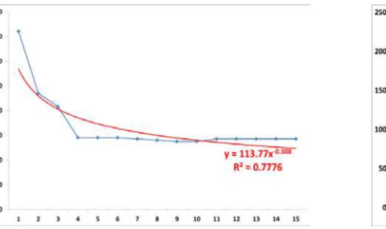
Designing a powerful algorithm depends on setting appropriate initial parameters of the solving method which are population size and generation number and mutation rate. Fig. 16 Shows the power-graphs for all examples, high value of r-square (�2) show high speed of solution convergence that is a consequence of employing backward and forward method which means the proposed method follows a logical way to find the optimal solution (or near optimal solution) and no illogical answer will reveal during the procedure of generation otherwise the amount of �2will significantly dropped.

Fig. 16. Power Graph for Backward-Forward Approach (examples 12 and 14)

30/2/ 20, 25 30/2/ 80, 70

Cmax Cmax

Generation Generation

50/5/ 80, 90, 90, 80, 90

50/5/ 20, 30, 20, 30, 40

(15)

Fig. 17. Comparing the Results of Serial Programming Method and the Proposed Method

Findings in Fig. 17 reveal that in all cases, BFSM can provide better feasible solution strings by moving activities through resource calendar. In addition, while RCPSPs are active which means one or more resources can be over allocated through the planning horizon in some time slots (problems 3, 5, 7, 9, 11 & 13), the amount of makespan saving is significantly less than relaxed RCPSPs where all resource constraints are relaxed (problems 2, 4, 6, 8, 10, 12 & 14).

Fig. 18. Impacts of Activity Splitting Ability on Minimizing Cmax in Studied Cases

Negative slope of graphs shows that using activity splitting ability allows managers to save �_�� significantly. In addition, by increasing number of activities and resources the degree of the slope which reveals speed of the convergence increases (Fig. 18).

Table 8

Results of Computational Experience

Ref. A RE RC Best Results (��) CPU

time

SP BFSM ∆�

Abbasi et al. (2006) 50 1 10 156 55 101 5.351

Shi-man et al. (2012) 8 4 9/20/20/20 51 29 22 0.751

Shi-man et al. (2012) 12 2 6/8 88 55 33 2.141

Wu et al. (2011) 27 3 6/6/6 89 63 26 2.57

For evaluating the performance of the proposed method, we used the performance measure called Makespan improvement that was proposed by Buddhakulsomsiri and Kim (2006):

��=��ℎ�� − ��ℎ��

��ℎ�� (18)

0 50 100 150 200 250

1 2 3 4 5 6 7 8 9 10 11 12 13 14

Cm

a

x

Experiments

Serial Pro. Method

The proposed method

0 20 40 60 80 100 120 140 160

MWS MW(O)S

(16)

Using makespan improvement ratio (Table 9), a supreme improvement can be seen while activity splitting is allowed which means that BFSM-GA can effectively use unfilled resource capacities respecting to activity priorities. Note that for the first problem, since both states of makespan with and without activity splitting reported the same structure, the makespan improvement value reported 0.

Table 9

Results of Comparing BFSM-GA with Serial Programming Method

No. A/R Resource capacity M.W.S M.W(O).S Makespan Improvement

1 6/3 8/10/8 14 14 0.00

3 10/2 10/10 21 32 0.34

5 15/2 20/11 29 54 0.46

7 18/3 15/20/10 57 79 0.278

9 20/3 15/20/10 53 91 0.417

11 30/2 20/25 55 144 0.618

13 50/5 20/30/20/30/40 79 128 0.383

A: Activity R: Resource

M.W.S: Makespan with activity splitting M.W (O).S: Makespan without activity splitting

Table 10

Results of Evaluating the Problems Gained from the Literature Using Proposed Method

No. References M.W.S M.W(O).S Makespan Improvement

1 Abbasi et al. (2006) 156 55 0.647

2 Shi-man et al. (2012) 51 29 0.431

3 Shi-man et al. (2012) 88 55 0.375

4 Wu et al. (2011) 89 63 0.292

In this comparison, results obtained by the competing algorithms have been taken verbatim from opted references from literature (Table 8). Results of the makespan ratio, it can be concluded that almost in all case the proposed method can provide supreme solutions. Using unfilled resources BFSM-GA can save

�� in a range between 27% and 64% depending on precedence matrix and resource availabilities

(Table 9 and Table 10). Moreover, the method is always promised to stay in feasible area through improving�_��. For future work, further attempt is suggest to solve the proposed model in multi-mode state (MRCPSP) using the proposed method.

5. Conclusion

By presenting the mixed backward-forward rescheduling technique, a novel mathematical method was developed to assure that, given the need to assign activities using remained resources through resource calendar while activity spitting is allowed, their combination will be as efficient as possible to minimize the makespan. Our finding show that using hybrid greedy and genetic algorithms for the proposed mixed backward-forward technique, where activity splitting is allowed, will cause noticeable reduction of makespan in classical RCPSPs that is a direct consequence of rising up in remained resources usage through project planning horizon.

Acknowledgment

(17)

References

Abbasi, B., Shadrokh, S., & Arkat, J. (2006). Bi-objective resource-constrained project scheduling with robustness and makespan criteria. Applied Mathematics and Computation, 180(1), 146-152.

Achuthan, N., & Hardjawidjaja, A. (2001). Project scheduling under time dependent costs–A branch and bound algorithm. Annals of Operations Research, 108(1-4), 55-74.

Alcaraz, J., & Maroto, C. (2001). A robust genetic algorithm for resource allocation in project scheduling.

Annals of Operations Research, 102(1-4), 83-109.

Buddhakulsomsiri, J., & Kim, D. S. (2006). Properties of multi-mode resource-constrained project scheduling problems with resource vacations and activity splitting. European Journal of Operational Research, 175(1), 279-295.

Castejón-Limas, M., Ordieres-Meré, J., González-Marcos, A., & González-Castro, V. (2011). Effort estimates through project complexity. Annals of Operations Research, 186(1), 395-406.

Chtourou, H., & Haouari, M. (2008). A two-stage-priority-rule-based algorithm for robust resource-constrained project scheduling. Computers & industrial engineering, 55(1), 183-194.

Delgoshaei, A., Ariffin, M. K., Baharudin, B. H. T. B., & Leman, Z. (2014). A Backward Approach for Maximizing Net Present Value of Multi-mode Pre-emptive Resource-Constrained Project Scheduling Problem with Discounted Cash Flows Using Simulated Annealing Algorithm. International Journal of Industrial Engineering and Management, 5(3), 151-158.

Demeulemeester, E. L. (2002). Project scheduling: a research handbook (Vol. 102): Springer.

Hartmann, S. (2001). Project scheduling with multiple modes: a genetic algorithm. Annals of Operations Research, 102(1-4), 111-135.

Hartmann, S., & Briskorn, D. (2010). A survey of variants and extensions of the resource-constrained project scheduling problem. European Journal of Operational Research, 207(1), 1-14.

Icmeli, O., Erenguc, S. S., & Zappe, C. J. (1993). Project scheduling problems: a survey. International Journal of Operations & Production Management, 13(11), 80-91.

Ke, H., & Liu, B. (2010). Fuzzy project scheduling problem and its hybrid intelligent algorithm. Applied Mathematical Modelling, 34(2), 301-308.

Kelley, J. E. (1963). The critical-path method: Resources planning and scheduling. Industrial scheduling, 13, 347-365.

Kim, K., Yun, Y., Yoon, J., Gen, M., & Yamazaki, G. (2005). Hybrid genetic algorithm with adaptive abilities for resource-constrained multiple project scheduling. Computers in industry, 56(2), 143-160. Kolisch, R. (1996). Serial and parallel resource-constrained project scheduling methods revisited: Theory

and computation. European Journal of Operational Research, 90(2), 320-333.

Kolisch, R., & Hartmann, S. (1999). Heuristic algorithms for the resource-constrained project scheduling problem: Classification and computational analysis: Springer.

Laslo, Z. (2010). Project portfolio management: An integrated method for resource planning and scheduling to minimize planning/scheduling-dependent expenses. International Journal of Project Management, 28(6), 609-618.

Lee, C.-Y., & Lei, L. (2001). Multiple-project scheduling with controllable project duration and hard resource constraint: some solvable cases. Annals of Operations Research, 102(1-4), 287-307.

Lombardi, M., & Milano, M. (2012). A min-flow algorithm for minimal critical set detection in resource constrained project scheduling. Artificial Intelligence, 182, 58-67.

Lova, A., & Tormos, P. (2001). Analysis of scheduling schemes and heuristic rules performance in resource-constrained multiproject scheduling. Annals of Operations Research, 102(1-4), 263-286. Patterson, J., Slowinski, R., Talbot, F., & Weglarz, J. (1989). An algorithm for a general class of

precedence and resource constrained scheduling problems. Advances in project scheduling, 187, 3-28.

(18)

Policella, N., Cesta, A., Oddi, A., & Smith, S. F. (2007). From precedence constraint posting to partial order schedules A CSP approach to Robust Scheduling. Ai Communications, 20(3), 163-180.

Seifi, M., & Tavakkoli-Moghaddam, R. (2008). A new bi-objective model for a multi-mode resource-constrained project scheduling problem with discounted cash flows and four payment models. Int. J. of Engineering, Transaction A: Basic, 21(4), 347-360.

Speranza, M. G., & Vercellis, C. (1993). Hierarchical models for multi-project planning and scheduling.

European Journal of Operational Research, 64(2), 312-325.

Sprecher, A. (2000). Scheduling resource-constrained projects competitively at modest memory requirements. Management Science, 46(5), 710-723.

Sprecher, A., Hartmann, S., & Drexl, A. (1997). An exact algorithm for project scheduling with multiple modes. Operations-Research-Spektrum, 19(3), 195-203.

Sung, C., & Lim, S. (1994). A project activity scheduling problem with net present value measure.

International Journal of Production Economics, 37(2), 177-187.

Talbot, F. B. (1982). Resource-constrained project scheduling with time-resource tradeoffs: The nonpreemptive case. Management Science, 28(10), 1197-1210.

Ulusoy, G., Sivrikaya-Şerifoğlu, F., & Şahin, Ş. (2001). Four payment models for the multi-mode resource constrained project scheduling problem with discounted cash flows. Annals of Operations Research, 102(1-4), 237-261.

Van de Vonder, S., Demeulemeester, E., Herroelen, W., & Leus, R. (2005). The use of buffers in project management: The trade-off between stability and makespan. International Journal of Production Economics, 97(2), 227-240.

Van de Vonder, S., Demeulemeester, E., Herroelen, W., & Leus, R. (2006). The trade-off between stability and makespan in resource-constrained project scheduling. International Journal of Production Research, 44(2), 215-236.

Yang, K. K., Talbot, F. B., & Patterson, J. H. (1993). Scheduling a project to maximize its net present value: an integer programming approach. European Journal of Operational Research, 64(2), 188-198. Yu, L., Wang, S., Wen, F., & Lai, K. K. (2012). Genetic algorithm-based multi-criteria project portfolio

selection. Annals of Operations Research, 197(1), 71-86.