Perturbações em torno de buracos negros e seus duais algébricos

(1)

UNIVERSIDADE DE SÃO PAULO

INSTITUTO DE FÍSICA

Perturbações em torno de Buracos Negros

e seus Duais Algébricos

Andrés Felipe Cardona Jiménez

Dissertação apresentada ao Instituto de Física da Universidade de São Paulo para a obtenção do título de Mestre em Ciências

Orientador: Prof. Dr. Carlos Molina Mendes

Banca Examinadora:

Prof. Dr. Carlos Molina Mendes (EACH/USP) Profa. Dra. Cecília Chirenti (CMCC/UFABC) Prof. Dr. George Matsas (IFT/UNESP)

São Paulo

(2)

FICHA CATALOGRÁFICA

Preparada pelo Serviço de Biblioteca e Informação

do Instituto de Física da Universidade de São Paulo

Cardona Jiménez, Andrés Felipe

Perturbações em torno de buracos negros e seus duais algébricos. São Paulo, 2015.

Dissertação (Mestrado) – Universidade de São Paulo. Instituto de Física. Depto. Física Matemática

Orientador: Prof. Dr. Carlos Molina Mendes

Área de Concentração: Gravitação

Unitermos: 1. Buracos negros; 2. Modos quase-normais; 3. Relatividade (Física)

(3)

UNIVERSITY OF SÃO PAULO

INSTITUTE OF PHYSICS

Perturbations around Black Holes

and their Algebraic Duals

Andrés Felipe Cardona Jiménez

A thesis submitted to the Physics Institute in partial fullfilment of the requirements for the degree ofMagister Scientiarum in Physics

Advisor: Prof. Dr. Carlos Molina Mendes

Examining Committee:

Prof. Dr. Carlos Molina Mendes (EACH/USP) Prof. Dr. Cecília Chirenti (CMCC/UFABC) Prof. Dr. George Matsas (IFT/UNESP)

São Paulo

(4)

To my beloved parents and grandma,

(5)

Acknowledgements

First of all, I would like to express my most sincere gratitude to my thesis advisor, Prof. Dr. Carlos Molina Mendes, for giving me the opportunity to work in this project, for his patience, motivation and continuous support.

Also I would like to thank my family: My parents Maria Elena and Jairo, and my grandmother Lucía, for their unconditional love and for support my decision of studying abroad, even if it meant a lot of worries for them. Without them I wouldn’t have made it this far.

To all my friends from Colombia, Brazil and other nationalities for the good moments shared together. I owe a special thanks to Daniel Morales and Javier Buitrago, for their kindness and for offering me their help when I first arrived at São Paulo.

To the CPG staff and the secretaries at the DFMA for their good attention and help.

(6)

Resumo

Nesta tese, nós estabelecemos algumas correspondências entre a dinâmica de campos escalares clássicos em certos espaço-tempos de fundo e duais algébricos apropriados. Os cenários estu-dados incluem soluções tipo buraco negro com constante cosmológica não nula e os

espaços-tempos conhecidos comogeometrias quase-extremas. Com base em várias propostas na

(7)

Abstract

In this thesis, we establish some correspondences between dynamics of classical scalar fields in certain background spacetimes and appropriate algebraic duals. The scenarios studied include

black hole solutions with non-zero cosmological constant and the spacetimes known as near

extremal geometries. Based on several proposals in the literature, we associate certain elements

(8)

List of Figures

3.1 Behavior ofr(r_∗)in near extremal SdS geometry. . . 30

3.2 Behavior ofr(r_∗)in near extremal wormhole geometry. . . 32

3.3 Behavior ofr(r_∗)of a black hole in compact geometry. . . 35

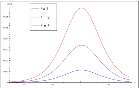
4.1 Effective potential for Schwarzschild-de Sitter spacetime as a function of the radial coordinate. Parametersr1=1,r2=10. . . 45 4.2 Effective potential for near extremal Schwarzschild-de Sitter as a function ofr_∗.

Parameters: r1=1,r2=1.05,ℓ=1. . . 47 4.3 Effective potential for Schwarzschild-Anti de Sitter spacetime as a function of

the radial coordinate for different event horizons in relation withR=1. . . 49

(11)

List of Tables

6.1 Lowest quasinormal modes and frequencies of the Pöschl-Teller potential. . . . 78

(12)

Chapter 1 Introduction

Black holes are one of the more interesting predictions of general relativity and understand-ing their properties is relevant for both astrophysical observations and the formulation of new physical theories. In the framework of general relativity, black holes are understood as compact objects, concentrating the largest amount of energy in the smallest possible volume; and their defining feature is the existence of an event horizon, a surface past which nothing can leave the black hole. In that sense black holes can be thought of as perfect black bodies since they always absorb but never radiate. In semi-classical approaches considering quantum fields on classical spacetime backgrounds, black holes are found to actually evaporate from the emission of thermal radiation with a characteristic temperature, called Hawking temperature, originating from quantum fluctuations at the event horizon. This led to a surprising connection between black hole physics and thermodynamics [1], in which black holes are the systems with the max-imum possible amount of entropy, proportional to the area of the event horizon, but also to some additional conceptual problems regarding the laws of quantum mechanics and the nature of Hawking radiation.

(13)

2

From the study of black hole perturbations we can gain insight on what we should look for in astronomical observations. The study of black hole perturbations goes back to the work of Regge and Wheeler [4] in the 50’s, where they studied the stability of the Schwarzschild black hole under perturbations. A classical treatment of the subject is given by Chandrasekhar [5], where scalar, electromagnetic and gravitational perturbations on the most familiar black hole scenarios are discussed, including the Schwarzschild, Reissner-Nordstrom and Kerr solutions.

An important characteristic of field perturbations are the so called quasinormal modes. After some transient period, perturbations outside the event horizon of a black hole are followed by oscillations with characteristic frequencies. This oscillations are exponentially damped, such that the associated frequencies, known as quasinormal frequencies, are complex. Quasinor-mal modes are important because they depend on the black hole properties, but not so much on the details of the initial perturbation. They can be thought of as resonances of the back-ground spacetime and it should be possible to characterize the nature of the black hole from the quasinormal frequencies. However, the analytic determination of quasinormal frequencies is not always possible. In fact, even for well-known geometries such as the Schwarzschild black hole, exact expressions for quasinormal frequencies are not available, and numerical methods or approximations are usually required. Revisions of the subject are found in Nollert [6], and Kokkotas [7], among other references.

The study of black hole perturbations and quasinormal modes has also acquired relevance for other reasons. A recent line of research in theoretical physics has been the pursue for corre-spondences between otherwise different physical theories, including the gauge/gravity dualities where, in principle, it could be possible to describe gravitational phenomena in terms of some gauge field theory which does not include gravitational interaction [8,9]. This approach is spe-cially meaningful if one of the theories is found to be difficult to solve but the dual theory is well understood. If these correspondences between gauge theories and gravity are valid, it should be possible to relate black hole perturbations with the correlations functions of a gauge theory.

The main feature of gauge field theories is the invariance of the dynamics under continuous local transformations, so every gauge theory is specified by a continuousLie group. Following

this line of thought, in recent works such as Castro el al., [10], Krishnan [11], Chen el al.

[12, 13], among others, it is suggested that in certain spacetimes and under specific limits, the dynamics of scalar fields is invariant under conformal transformations, establishing a direct relation with the quasinormal modes on those scenarios. These works are the base of this thesis and we aim to find further scenarios where we can apply this reasoning.

(14)

3

or a cosmological horizon, and a certain limit where both Killing horizons become arbitrarily close. The advantage of working with these spacetimes is that the scalar dynamics is greatly simplified, and they can be used to approximate more complicated scenarios. Our goal is to es-tablish a correspondence between perturbative quantities (quasinormal modes and spectrum of quasinormal frequencies) of certain geometries and algebraic elements associated with a repre-sentation of a conformal symmetry. In these scenarios, it should be possible to characterize the evolution of classical scalar perturbations with proper algebraic duals related to the invariance of the dynamics under conformal transformations, which in our case will be transformations under the special linear groupSL(2)and its algebrasl(2).

The outline of this thesis is as follows: In chapter 2 we present a review on the basic topics of general relativity, where we focus on how the symmetries of a spacetime are associated with Killing vectors. We introduce the ideas of staticity, stationarity and spherical symmetry, ultimately defining the concept of what a black hole is, with details of the most well known example: the Schwarzschild solution. In chapter 3 we introduce the relevant geometries for our thesis, which include the generalizations of the Schwarzschild solution to spacetimes with non-zero cosmological constant, namely the Schwarzschild-de Sitter and Schwarzschild-Anti de Sitter spacetimes. We also introduce properly the idea of near extremal geometries explored in the present work.

After having introduced the tools to study general relativity and the geometries of interest, in chapter 4 we proceed to discuss how perturbations of fields are treated on a background spacetime, in particular we develop on the dynamics of scalar fields on static and spherically symmetric spacetimes and we define the notion quasinormal modes and frequencies and their relevance for the evolution of a field perturbation.

In the last two chapters we treat the connection between field dynamics and algebra repre-sentations. In chapter 5 we introduce some details on group theory, focusing on Lie groups and representation theory of Lie algebras, and we eventually introduce the groupSL(2)and algebra

sl(2). Finally, in chapter 6 we present the results of our work, where we find a explicit represen-tation of the algebrasl(2)in terms of differential operators, from which we are able to obtain the spectrum of quasinormal frequencies for the near extremal geometries. We also present an-other representation which could be used to model the scalar dynamics in asymptotically Anti de Sitter spacetimes. Final comments and conclusions are presented in chapter 7.

(15)

Chapter 2 General Relativity

Einstein’s general relativity is currently the most widely accepted theory to describe the gravita-tional interaction and is central to the understanding of a great array of astrophysical phenomena such as black holes, gravitational waves, and the expansion of the universe [14], but remarkably, it is the only known interaction still resisting a consistent quantum mechanical description. For-mulated by Albert Einstein in 1915 as an effort to reconcile Newton’s gravitational theory with relativistic dynamics, general relativity treats gravity not as a force but as a consequence of a curved spacetime where matter and radiation act as the source of curvature [15, 16]. General relativity has been tested in the solar system matching with great accuracy with experimental observations, ranging from the correct prediction of perihelion precession of Mercury’s orbit, the deflection of light by massive bodies and the gravitational redshift of light [17].

General relativity is based upon two principles:

• Equivalence principle: Although there is not an unique consensus in the exact formulation

of this principle, at its heart, the equivalence principle states the impossibility for an observer to distinguish locally between an acceleration in his own reference frame and the effects of a gravitational field. The base of this principle is the equivalence between inertial and gravitational mass holding for every body, regardless of size or composition, [16].

• Principle of general covariance: This principle is based on the requirement for all physics

laws to have the same formulation in all reference frames, meaning that there is not such thing as a preferred reference frame. Moreover, special relativity should hold at least locally. The global Lorentz covariance of special relativity becomes a local Lorentz co-variance when gravity is introduced [18].

(16)

2.1 Elements of differential geometry 5

of that, it is not possible to define a real inertial observer able to properly measure effects of the gravitational field, as it will experience the effects of gravity as well [19,20].

2.1 Elements of differential geometry

The mathematical formalism used in general relativity is differential geometry, and spacetime, which is the main object of study, is described as a differentiable manifold. An informal idea of a manifold is a space that locally looks likeRnbut globally may posses a nontrivial structure. To provide a formal definition of a manifold some preliminary concepts are introduced :

• Given a set M, a chart(also called coordinate system) _{U,φ_} is a subsetU ofM along

with a one-to-one map φ :U _→Rn such that_φ_(U) is an open set in Rn, making_U an

open set inM[21,22].

• Anatlasis a collection of charts_{Ui,φi}such that (i) the union of the subsetsUicoversM

and (ii) if two charts overlap,Uα∩Uβ, the map(φα◦φβ−1)takes points inφβ(Uα∩Uβ)⊂

Rnonto an open set_φ_α_(U_α_∩_U_β₎_⊂Rn[21] .

The last requirement means that if two charts overlap in a certain region ofM, there must be

aC∞continuous coordinate transformation between both charts. With this concepts established

a more precise definition of the idea of manifold is the following: A smooth n-dimensional manifold is a set M along with a maximal atlas, that is, an atlas that contains every possible

compatible chart [15,20,22].

In general relativity spacetime is treated as a continuous, connected four dimensional mani-fold. A point in spacetime is called an event, with three spatial and one temporal coordinate. A coordinate system is by no means unique and physical quantities should be independent from a particular choice of coordinates .

To every point pof aM can be associated the set of tangent vectors of every curve passing

throughp. These vectors form a vector spaceV since they can be added together and multiplied

by scalars. The vector spaceV is called tangent space. To every smooth function f :M _→R can be associated a directional derivative with respect to a curveγ passing through p; if such

curve is parameterized by a certainλ _∈R, the directional derivative of _f is given by df

dλ =

dxµ

(17)

where_{∂µ}are partial derivatives with respect to some coordinate chart{xµ}. Since f is taken

to be an arbitrary function, the directional derivative operation is given by

d

dλ =

dxµ

dλ ∂µ, (2.2)

therefore_{∂µ}represent a basis for the vector space of directional derivative operators along

curves through p, and thus, of the tangent spaceTp. This kind of basis is known as coordinate

basis; elements of this basis are in general not normalized to unity nor orthogonal to each other.

If_{∂µ}is a basis for the tangent space at p, any elementV ∈Tpcan be written asV =Vµ∂µ.

According to the chain rule of partial derivatives,_{∂µ}transforms under a change of coordinates

xµ _→xµ′as

∂µ′= ∂x

µ

∂xµ′∂µ, (2.3)

thus, forV to remain invariant under this transformation, the componentsVµ must transform in

the following manner

Vµ′= ∂x

µ′

∂xµV

µ_. _(2.4)

If the components of a vectorV transform as (2.4),V is said to be a contravariant vector. Given

two vector fieldsX,Y, it is defined the Lie bracket[X,Y]as

[X,Y]f _≡X(Y(f))₋Y(X(f)) (2.5)

which in components is

[X,Y]µ =Xν∂νYµ−Yν∂νXµ. (2.6)

To every tangent space it can be associated the cotangent spaceT_p∗ as the set of linear maps

ω :Tp→R. If elements ofTp are identified with directional derivatives of a function f in p,

elements onT_p∗ can be identified with the gradient df of such function. Following the same

argument, just as partial derivatives_{∂µ}with respect to the coordinate functionsxµ constitute

a basis forTp, the gradients{dxµ}of the coordinatesxµ provide a basis for the cotangent space T_p∗.

Any element of T_p∗ can be expanded asω =ωµdxµ. Since under a change of coordinates

xµ _→xµ′gradients transform as

dxµ′= ∂xµ′

∂xµ

dxµ, (2.7)

the componentsωµ must transform as

ωµ′= ∂xµ

(18)

forω to remain unchanged under this transformation. Elements ofT_p∗whose components

trans-form as (2.8) are known as covariant vectors or one-forms.

A generalization of the notion of vectors and dual vectors is the idea of tensor. A tensorT of

rank(k,l)is a multilinear map fromkcopies of the cotangent space andl copies of the tangent

space toR,

T :Tp⊗ ··· ×Tp

| {z }

kcopies

×T_p∗_{× ··· ×}T_p∗

| {z }

lcopies

→R_. (2.9)

In components, an arbitrary tensorT can be written as

T =Tµ1...µk

ν1...νl∂µ1⊗ ··· ⊗∂µkdx

ν1_{⊗ ··· ⊗}_d_xνl_. (2.10)

Tensors are important in general relativity because a tensorial equation valid in a coordinate system will be valid in every other coordinate systems, as implied the principle of general covariance, suggesting that every equation describing physical quantities should be written in terms of tensors.

A tensor of fundamental importance in general relativity is the metric tensor, a symmetric

(0,2)tensor whose components are denoted asgµν. This tensor allows to generalize the notion

of Euclidean distance and scalar product of vectors inRn to arbitrary curved manifolds. For two vectorsV andW the scalar product(V,W)is defined as

(V,W) =gµνVµWν, (2.11)

where the line element dsis defined as

ds2=gµνdxµdxν. (2.12)

The metric tensor allows to determine of the path length between two points in a manifold, therefore providing a generalization of distance. The metric tensor generalizes the idea of vector norm as well, defined as the scalar product of the vector with itself

In general relativity the signature of the metric is(₋,+,+,+)(the signature are the signs of the eigenvalues of the metric). Manifolds with this metric signature are called pseudo-Riemannian or Lorentzian manifolds. In a pseudo-pseudo-Riemannian metric the norm of a vector is not positive-defined, and vectors are classified according to the value of the norm

(V,V) =gµνVµVν

  

 

<0 V is timelike

=0 V is null

>0 V is spacelike

(19)

This classification also applies to curves and surfaces: A timelike/null/spacelike curve is a curve whose tangent vector is timelike/null/spacelike at every point, and a timelike/null/spacelike surface is a surface whose normal vector is timelike/null/spacelike everywhere. The type of curve that a particle follows through spacetime depends on its mass: massive particles move along timelike curves while massless particles move move along null curves [15,16].

Since general relativity generalizes Minkowski spacetime to arbitrarily curved Lorentzian spacetimes, the metric tensor also provides a notion of causality. In Minkowski spacetime a light cone, which is the path that a light beam emanating from a single event and traveling in all directions would take, has the same shape at every spacetime point. The same does not hold for an arbitrarily curved spacetime, instead, in general relativity it is said that two events are causally related if they can be connected by a causal curve, that is, a curve that is null or timelike everywhere.

2.1.1 Curvature

In a curved spacetime a generalization of partial derivatives must be introduced since, in gen-eral, tangent spaces at different points are not equal and thus, a direct comparison of vectors at different points is not plausible. One such generalization is the covariant derivative∇, an operator mapping(k,l)tensors to (k,l+q) tensors. As a generalization of partial derivatives, covariant derivatives should satisfy the properties characterizing a differential operator

1. Linearity: ∇(X+Y) =∇X+∇Y .

2. Leibniz rule: ∇(X_⊗Y) = (∇X)_⊗Y+X_⊗(∇Y) .

The covariant derivative of a contravariant vectorV and a covariant vectorω are respectively (in component notation)

∇_µVν=∂µVν+ΓνµλVλ, (2.14)

∇_µων=∂µων−Γλµνωλ, (2.15)

whereΓν_µλ are called connection coefficients. These coefficients allows us to compare vectors

between tangent spaces of nearby points. It can be shown that the connection coefficients do not transform as tensor components, however, the covariant derivative does have the transformation properties of a tensor [15],

∇_µ′Vν′= ∂x

µ

∂xµ′

∂xν′

∂xν ∇µV

(20)

To every connection can be associated a tensor knows as the torsion tensor

Tλµν =Γλµν−Γλν µ. (2.17)

The connection coefficients are not unique, as they depend on the procedure employed to com-pare vectors at different tangent spaces. Nevertheless for every manifold there is a unique connection such that the covariant derivative of the metric with respect to that connection is zero at every point,∇_µgµν =0, and the associated torsion tensor is zero. This unique, metric

compatible connection, is found to be expressed in terms of the metric components and their first order derivatives

Γσ_µν = 1

2g

σ ρ _∂

µgνρ+∂νgρ µ−∂ρgµν, (2.18)

and it is known as Christoffel connection. In general relativity it is usually assumed a metric compatible connection and a vanishing torsion tensor.

Contrary to the case of partial derivatives, covariant derivatives with respect to different coordinates do not commute; and it is precisely through this non-commutative behavior that the idea of curvature can be quantified. The commutator of covariant derivatives with respect to two different coordinates acting on a vectorV is, in component notation,

[∇_µ,∇_ν]Vρ =Rρσ µνVρ−Tλµν∇λVρ, (2.19)

whereTλµν is the torsion tensor (2.17). The fist term defines a tensor of significant importance

known as the Riemann tensor, a (1,3) rank tensor whose components are given by

Rρσ µν=∂µΓρνσ−∂νΓρµσ+ΓρµλΓλνσ−ΓρνσΓλµσ. (2.20)

If a coordinate system exists such that the components of the metric tensor are coordinate inde-pendent, the Riemann tensor will vanish. Another important tensor, known as the Ricci tensor, is defined from the Riemann tensor by contraction of index

Rµν =Rλµλ ν. (2.21)

The trace of the Ricci tensor is called the Ricci scalar or curvature scalar and it is a quantity that remains invariant under coordinate changes

(21)

In the absence of gravity, that is, in flat spacetime, particles move in straight lines. In curved spacetimes a generalization of straight line is the idea of geodesic, as the path of shortest dis-tance between two points. A pathxµ(τ), whereτ is a parameter of motion, is a geodesic if the

tangent vector dxµ/dτ satisfies

dxµ

dτ ∇µ

dxν

dτ =0, (2.23)

which in terms of the covariant derivative (2.14) is known as the geodesic equation

d2xµ

dτ2 +Γ

µ αβ

dxα

dτ

dxβ

dτ =0. (2.24)

The world line of a particle free from all external, non-gravitational force, is a particular type of geodesic. In other words, a freely moving or falling particle always moves along a geodesic.

2.1.2 Diffeomorphims

Two manifoldsM andN, not necessarily of the same dimension, can be related by some map

ϕ:M_→N, a rule assigning to each element ofMexactly one element ofN. If such map exists,

a linear map between tangent spaces in both spaces is induced. More precisely, for somep_∈M,

a linear map

ϕ∗:TpM_→Tϕ(p)N, (2.25)

from the tangent space ofM at p to the tangent space of N at ϕ(p). If v_∈Tp(M), the vector

ϕ_∗v_∈T_ϕ₍_p₎Nis called the pushforward ofvbyϕ. Vectors as defined by their action on functions as directional derivatives. If there is a function f :N _→Rthe action of_ϕ_∗_von _f is defined to be equivalent to the action ofvon the composition f_◦ϕ∗:M_→R,

(ϕ∗v) (f) =v(f_◦ϕ), (2.26)

where “_◦” indicates composition of maps. Likewise, there is an associated linear map between cotangents spaces, relating dual vectors fromT_ϕ∗₍_p₎(N)to dual vectors inT_p∗(M)

ϕ_∗:T_ϕ∗₍_p₎N_→T_p∗(M), (2.27)

ifω _∈T_ϕ∗₍_p₎N the pullback one formϕ_∗ωµ is defined requiring that for allv∈Tp(M)

(22)

IfMhas coordinates_{xµ_}andN has coordinates_{yα_}the components of a vectorv_∈TpMand

the pushforward vector(φ∗v)_∈T_ϕ₍_p₎N are related by (φ∗v)α =vµ∂y

α

∂xµ, (2.29)

therefore, it is possible to think of a pushforward as a matrix operator of the form

(ϕ∗v)α = (ϕ_∗v)α_µvµ with components given by the Jacobian matrix of the map ϕ between coordinates

(ϕ∗)α_µ =∂y

α

∂xµ. (2.30)

SinceMandN are not necessarily of the same dimension, this pushforward matrix is in general

not invertible.

If a mapϕ:M_→Nbetween two manifoldsMandNisC∞is one-to-one and its inverseϕ−1:

N_→MisC∞, the mapϕis said to be a diffeomorphism. In that caseMandNare necessarily of

the same dimension, and are said to be diffeomorphic. In particular, the pushforward operation turns out to be invertible.

IfMandNare the same manifold, a diffeomorphism induces a change of coordinate system:

Ifxµ :M_→Ris a coordinate function defined on _M it is possible to define a new coordinate system by(ϕ∗x)µ :M_→Rn. This transformation be seen as moving the points of the manifold and evaluate the coordinates at the new points, called active coordinate transformations, con-trary to passive coordinate transformations, where new coordinates are introduced as functions of the previous ones.

2.1.3 Lie derivative

Diffeomorphims also provide another alternative to compare vectors at different spacetime points using the operations of pullback and pushforward, and thus, allowing to define another differential operation. It is required a family of diffeomorphism_{ϕt}parameterized byt∈R.

The action of_{ϕt}on a point pinMwill describe a curvexµ(t)parameterized byt. The action

of _{ϕt} on every point will generate a set of curves covering M entirely. The set of tangent

vectors to each curve at each point defines a vector fieldVµ(x),

dxµ dt =V

µ_. _(2.31)

It is possible to find the variation rate of a tensorT along the vector fieldV as the difference

be-tween the pullback of the tensor from a pointqto pand its original value at point p. Since both

(23)

the tensor along a vector fieldV

L_V_Tµ1µ2...

ν1ν2...=lim

t→0

ϕ_t∗[Tµ1µ2..._ν

1ν2...(ϕt(p))]−Tµ1µ2...ν1ν2...(p)

t . (2.32)

Lie derivative is a mapping from tensor fields(k,l)to(k,l)manifestly independent of the coor-dinate system. This operation is linear and satisfies the Leibniz rule:

L_V_(aT₊_{bS) =}_aL_V_T₊_bL_V_S_, (2.33)

L_V_(T_⊗_{S) = (}L_V_T₎_⊗_S₊_T_⊗₍L_V_S)_. (2.34)

Lie derivative of scalar functions is equivalent to an ordinary directional derivative

L_V _f ₌_V₍_f_{) =}_Vµ_∂_µ_f_. (2.35)

To determine the action of the Lie derivative on tensors it is convenient to chose a coordinate systemxµ= (x1, . . .xn)such thatx1is the parameter along the curves. In that caseV =∂/∂x1

with componentsVµ = (1,0, ...,0). A diffeomorphism by t is equivalent to a transformation xµ _→yµ= (x1+t,x2, ...)and the pullback matrix is

(ϕ_t∗)µν =δµν. (2.36)

In this new coordinate system the Lie derivative becomes

L_V_Tµ1...µk

ν₁...νk=

∂ ∂x1T

µ1...µk

ν₁...νk. (2.37)

For a vector fieldUµ

L_VUµ ₌ ∂

∂x1U

µ_. _(2.38)

This expression is not covariant, but it is equivalent in this coordinate system to the Lie bracket

[V,U]between two vector fieldsV andU

[V,U]µ=Vν∂νUµ−Uν∂νVµ. (2.39)

Since the Lie bracket is a well-defined tensor the Lie derivative of a vector fieldUalong a vector

fieldV is given in any coordinate system by the Lie bracket between both vectors

(24)

In general, for an arbitrary tensorTµ1...µkν1...νkthe Lie derivative can be written as [15]

L_V_Tµ1...µk

ν₁...νk =V

σ₍_∇

σTµ1...µkν₁...νk)

−(∇_λVµ1_)Tλ...µk

ν1...νk−. . .−(∇λV

µk_)Tµ1...λ

ν1...νk

+ (∇_ν₁Vλ)Tµ1...µk

λ...νk+. . .+ (∇νlV

λ_)Tµ1...µk

ν₁...λ.

(2.41)

In particular, the Lie derivative of the metric tensor is

L_V_g_µν ₌_Vσ_∇_σ_g_µν_{+ (}_∇_ν_Vλ_)g_{λ ν}_{+ (}_∇_ν_Vλ_)g_µλ

=∇_µVν+∇νVµ,

(2.42)

where it has been used the fact that∇_σgµν =0 if ∇µ is the covariant derivative associated to

the metric affine connection ofgµν.

2.1.4 Symmetries and Killing vectors

A manifoldM is said to posses a symmetry if under a certain transformation of the manifold

into itself there are quantities remaining invariant. In particular, if the transformation is a dif-feomorphismϕ, a tensorT is invariant if it remains unchanged under the pullback ofϕ

ϕ∗T =T. (2.43)

If the symmetry is generated by a family of diffeomorphismsϕt related to a vector fieldVµ then

the Lie derivative ofT over the flow ofV will be zero

L_V_(T_{) =}0_. (2.44)

This implies that it is always possible to find a coordinate system in which the components of

T are independent of one of the coordinates (the coordinates of the integral curves of the vector

field).

If the metric tensorgµν ofMis invariant under a diffeomorphismϕ, that is,ϕ∗gµν =gµν,

thenϕ is called an isometry. If the isometries are generated by a vector fieldKµ then

L_Kg_µν₌0_, (2.45)

or from equation (2.42)

∇_µKν+∇νKµ=0. (2.46)

(25)

2.2 Einstein’s field equations 14

Killing vectors define a conserved currentJµ=KνTµνsuch that∇µJµ =0 [15]. If a spacetime

has a Killing vector, it is always possible to find a coordinate system in which the metric is independent of one of the coordinates

2.2 Einstein’s field equations

The central idea of general relativity is the association between gravity and spacetime geometry, in particular, the relation between curvature of spacetime and the energy and momentum of any form of matter and radiation present. The content of energy momentum is described by a second rank contravariant tensorTµν known as the energy-momentum tensor, satisfying the

mass-energy conservation condition [16,19],

∇µTµν =0. (2.47)

To establish such relation between matter with curvature it is necessary to find a second rank contravariant tensor built from the metric tensor and its derivatives and satisfying the divergen-less condition. Even though the Ricci tensor is a second rank tensor containing information of curvature, it is not a good choice since, in general, is not divergenless. However, from both the Ricci tensor (2.21) and the curvature scalar (2.22) a tensorGµν satisfying the divergenless

condition∇µGµν =0 is found

Gµν =Rµν−

1

2Rgµν, (2.48)

and it is called Einstein’s tensor. Thus, Einstein’s field equations are formulated as a directly proportional relation betweenGµν andTµν

Rµν−1

2R gµν = 8πG

c4 Tµν, (2.49)

Einstein’s field equation constitute a system of 10 independent non-linear differential equations whose solutions are the components of the metric tensor, representing the gravitational field. This equations reduce to Newton’s gravitation law

∇2Φ=4πGρ, (2.50)

in the limit of weak gravitation field and low motion [16].

Einstein’s equation can be modified to include an additional term proportional to the metric

Rµν−1

2R gµν+Λgµν= 8πG

(26)

2.3 Spherically symmetric and maximally symmetric spacetimes 15

This additional term can be thought of as an additional component of the energy-momentum tensor

T_µν′ =Tµν−

Λc4

8πGgµν, (2.52)

The constantΛis called cosmological constant and it commonly interpreted as the energy den-sity of empty space. A useful form of Einstein’s equation involve taking trace in (2.49)

Rµν=

8πG c4

Tµν−

1 2T gµν

, (2.53)

such that vacuum solutions are obtained by solvingRµν=0. Einstein’s equation can be derived

using a variational method from the Einstein-Hilbert action:

SEH = 1

16πG

Z

d4x√₋g(R₋2Λ) +Smatter, (2.54)

whereSmatter is the action of whatever matter is present content, whose variation with respect

to the metric defines the energy momentum tensor

Tµν=−√2

−g

δSmatter

δgµν

. (2.55)

The Einstein-Hilbert action is the only possible action if invariance under change of coordinates is demanded and involving at most second order derivatives of the metric tensor components [15].

2.3 Spherically symmetric and maximally symmetric

space-times

Given the non-linear character of Einstein’s field equations it is not possible to obtain a general solution. Most known solutions suppose a certain number of symmetries and/or simplifications. Among the most relevant symmetries usually considered are

• Spherical symmetry: In a spherically symmetric spacetime there is no preferred spatial

direction. A coordinate-independent property of spherically symmetric spacetimes is the existence of three spacelike, linearly independent killing vector fields _{Vi}3i=1 satisfying the algebra of the groupSO(3)

[Vi,Vj] =εi jkVk, i,j,k=1,2,3. (2.56)

(27)

• Stationarity: Informally, stationarity means no explicit time dependence. A stationary

spacetime is characterized by possessing a vector field which is globally timelike. In a a coordinate system(t,x1,x2,x3)the associated Killing vector is denoted∂t with

compo-nents_{∂t}µ = (1,0,0,0).

• Staticity: In a non rigurous way, a physical system is static if it does not evolve over

time. A spacetime is static if all of the metric components are time independent and invariant under temporal reflection (crossed terms of the form dtdxi or dxidt are absent).

Static spacetimes are characterized in a coordinate independent way by the existence of a timelike killing vector field orthogonal to a family of spatial hypersurfaces parameterized byt constant. A timelike killing vector xµ is orthogonal to a hypersurface if it satisfies

the following equation

x_[_µ∇_νx_σ_]=0, (2.57)

which is a result following from the well known Frobenius’s Theorem (the braces are a notation indicating an antisymmetric, linear combinations of terms with index permuta-tion) for details see for example appendix B of [19].

In a spherically symmetric and static spacetime the metric tensor can be described by a coor-dinate system(t,r,θ,φ), wheret is a temporal coordinate associated with the timelike Killing

vector defining staticity and(θ,φ)are the usual spherical coordinates parameterizing surfaces

invariant under rotations (surfaces with areaA=4πr2). In this coordinate system the metric

tensor can be casted as

ds2=₋A(r)dt2+ 1 B(r)dr

2₊_r2_d_Ω2_, _(2.58)

where

dΩ2= dθ2+sin2θdφ2, (2.59)

is the line element of the 2-sphere andA(r) andB(r) are functions depending only on r and

should be positive definite in the case of Lorentzian manifolds. It should be noted that the struc-ture of the metric tensor (2.58) is not obtained from solving Einstein’s field equation but rather from considering the most general metric satisfying the conditions of staticity and spherical symmetry [15].

The causal structure of a spacetime is dictated by the behavior of light cones, which can be obtained from the set of radial null curves, that is, curves for which ds2 =0 and θ,φ are constant. For metrics of the form (2.58) such those curves are given by

dt

dr =±

1

p

(28)

which is equivalent to the geodesics of massless particles obtained from solving the geodesic equation (2.24)

dt

dτ =

1

p

A(r)B(r) and

dr

dτ =±1. (2.61)

In Minkowski spacetime dt/dr=_±1, that is, light cones form a angle of 45 degrees at every

point. However, equation (2.60) indicates that if the metric coefficients depend onr the light

cones slope will be different at each point of spacetime. Motivated from this observation, it is convenient to define a new coordinater_∗, called tortoise coordinate, by

dr_∗

dr =

1

p

A(r)B(r), (2.62)

such that the temporal coordinatetand the new tortoise coordinate are related in the form

t=_±r_∗+ constant , (2.63)

implying that for radial null curves dt =_±dr_∗. In the coordinate system (t,r_∗,θ,φ)the metric

(2.58) becomes

ds2=A_(r_∗₎ ₋d_t2₊d_r_∗2₊_r2_(r_∗₎d_Ω2_, (2.64)

whereA_(r_∗_{) =}_A(r(r_∗₎₎. In this particular coordinate system_(t_,_r_∗_,_θ_,_φ₎the metric is

charac-terized by the functionsA_(r_∗₎and_r(r_∗₎.

Another important coordinate systems are based on the advanced timeuand retarded time

v, defined as

u=t₋r_∗, (2.65)

v=t+r_∗. (2.66)

Null geodesics withu constant satisfy dt=dr_∗whereas null geodesics withvconstant satisfy

dt =₋dr_∗. The coordinate systems(u,r,θ,φ) and(v,r,θ,φ)are called ingoingandoutgoing Eddington-Finkelstein coordinates respectively [23]. In the coordinate system (v,r,θ,φ), the metric (2.58) adopts the following form

ds2=₋A(r)dv2+

s

A(r)

B(r)(dvdr+drdv)r

2_d_Ω2_, _(2.67)

while in the coordinate system(u,r,θ,φ)a similar expression is obtained

ds2=₋A(r)du2₋

s

A(r)

B(r)(dudr+drdu) +r

(29)

It is possible to define another coordinate system using both the retarded and advanced times

u,v. From the form of the metric tensor in the coordinates (t,r_∗,θ,φ)given by (2.64) and the

replacements

t= 1

2(u+v), r∗= 1

2(v−u). (2.69)

we get the following expression for the metric

ds2=₋A_(r_∗_(u_,_v))d_ud_v₊_r2_(r_∗_(u_,_v))dΩ2, (2.70) with the particularity that there are no quadratic terms in du or dv. The coordinates (u,v)are

well suited to describe radial null geodesics, since the condition ds2=0 implies that massless particles propagate at eitheruconstant orvconstant, which are null curves.

2.3.1 Maximally symmetric spacetimes

Ann-dimensional manifold with1₂n(n+1)Killing vectors is said to be a maximally symmetric

space, that is, a space with the maximum number of possible isometries. For a maximally symmetric space the curvature is constant everywhere, and the Riemann tensor is [15]

Rµνρσ =

R

n(n₋1) gµρgνσ−gµσgνρ

. (2.71)

Maximally symmetric spaces are characterized locally by the value of the Ricci tensorR,

clas-sified according to whetherRis positive, negative or zero. For Euclidean spacesR=0 corre-sponds toRn,_R_>0 corresponds to_Snand_R_<0 corresponds to an_n-dimensional hyperboloid.

For Lorentzian manifolds the maximally symmetric spacetime with R=0 is Minkowski

space, which in addition to static and spherical symmetries possesses Poincaré invariance under Lorentz boosts and translations. Likewise, the maximally symmetric space with positive cur-vature is known as de Sitter spacetime (dS) and the negative curcur-vature spacetime is called Anti de Sitter spacetime (AdS). These two geometries are solutions to the Einstein’s equation with non-zero cosmological constant (2.51).

de Sitterspacetime is the vacuum solution to Einstein’s field equation with positive

cosmo-logical constant, Λ>0. In four dimensions and it a coordinate system (t,r,θ,φ), the metric tensor of de Sitter spacetime is of the form (2.58) with [24]

A(r) =B(r) =1₋Λr2

(30)

or, equivalently

ds2=₋

1₋r2

a2

dt2+

1₋r2

a2

−1

dr2+r2dΩ2, (2.73)

wherea=p3/Λ is called the de Sitter radius. As a particular feature, the metric component

grr=B(r)−1 becomes singular at r=a andA(r),B(r)<0 for r>a. The domain of validity

of the radial coordinate isr_∈[0,a), in which the functionsA(r)andB(r)are positive defined.

The surfacer=ais said to be acosmological horizon, a surface surrounding any observer and

delimiting the space from which the observer can retrieve information. The tortoise coordinate of de Sitter spacetime is given by

dr_∗

dr =

1₋Λr2 3

−1

. (2.74)

The solution of this equation is

r_∗(r) =

r 3 Λtanh −1 r Λ 3r ! . (2.75)

Thus, the original domain of the radial coordinate r is extended to r_∗ _∈[0,∞). The tortoise coordinater_∗(r)can be inverted analytically, giving functionsr(r_∗)andA_(r_∗₎as a function of

r_∗

r(r_∗) =

r

3

Λtanh r

Λ

3r∗

!

, (2.76)

A_(r_∗_{) =} r

3

Λsech r

Λ

3r∗

!

. (2.77)

The expression for the metric in(t,r_∗,θ,φ)coordinates is ds2=sech2r∗

a

−dt2+dr_∗2+a2tanh2

_r_∗

a

dΩ2. (2.78)

Anti de Sitter spacetime is the maximally symmetric solution of Einstein’s equation with

negative cosmological constant Λ, corresponding to a negative vacuum energy density and

positive pressure. In the coordinate system(t,r,θ,φ) the AdS metric is characterized by the

functions

A(r) =B(r) =1+Λr

2

(31)

whereΛ=₋3/R2<0. In this case the line element is [25]

ds2=₋

1+ r

2

R2

dt2+

1+ r

2

R2

−1

dr2+r2dΩ. (2.80)

The metric tensor is well-defined forr_∈[0,∞). Anti de Sitter resembles Minkowski spacetime

forr_≪Rbut has a different asymptotic behavior nearR. The tortoise coordinate is given by

dr_∗

dr =

1+ r

2

R2

−1

, (2.81)

with solution

r_∗(r) =Rarctan

_r

R

. (2.82)

The tortoise coordinate can be inverted; and the functionsr(r_∗)andA_(r_∗₎are given by

r(r_∗) =Rtan

_r

∗

R

, (2.83)

A_(r_∗_{) =}sec2r∗

R

. (2.84)

The expression for the metric in(t,r_∗,θ,φ)coordinates is

ds2=sec2r∗ R

−dt2+dr_∗2+R2tan

_r_∗

R

2

dΩ2_. (2.85)

The Anti de Sitter spacetime shares very interesting features, and it plays a prominent rule in the AdS/CFT correspondence, first introduced in [26], which has been a very active line of

research over the last decade. For example, even though there is a well defined limitr_→∞,

AdS has the property that a light beam emitted from any point can reach spatial infinity and

(32)

2.3.2 Schwarzschild spacetime

A well studied solution of Einstein’s equations is the Schwarzschild spacetime [27], which is the unique, spherically symmetric and static vacuum describing spacetime outside a spherical object of massM. In coordinates(t,r,θ,φ)the Schwarzschild metric is is given by

A(r) =B(r) =

1₋2M

r

, (2.86)

with corresponding line element

ds2=₋

1₋2M

r

dt2+

1₋2M

r

−1

dr2+r2dΩ2. (2.87)

In this coordinate system the metric tensor presents two divergences: The component grr

be-comes singular at r =2M; it is well known that this divergence is not physical and can be

removed by choosing a more appropriated coordinate system [15]. The other divergence cor-responds to the componentgtt atr=0. This is a physical singularity, since certain coordinate invariant quantities, such as the Kretschmann invariantRµνρσRµνρσ, becomes singular at that

point

RµνρσRµνρσ = 48

G2M2

r6 . (2.88)

Thereforer=0 should not be considered as part of the manifold, even though it can be reached from other points.

Even though r=2M is a regular surface, the coordinate system (t,r,θ,φ) is only mean-ingful for the regionr>2M. A more appropriated coordinate system is given by the tortoise

coordinater_∗, defined by (2.62). For Schwarzschild spacetime the tortoise coordinate is

dr_∗

dr =

1₋2M

r

−1

, (2.89)

which can be integrated to yield

r_∗(r) =r+2Mln

_r

2M−1

. (2.90)

The domain of the radial coordinater_∈(2M,∞)is extended tor_∗_∈(₋∞,∞), with the surface r=2Mpushed tor_∗_{→ −}∞. It is to be noted that equation (2.90) cannot be inverted analytically

to yieldras a function ofr_∗. From the tortoise coordinate (2.90) the retarded and advanced times

are obtained. In the ingoing Eddington-Finkelstein coordinates(v,r)and(u,r)the metric tensor takes the form

ds2=₋

1₋2M

r

(33)

2.4 Black holes 22

while in the outgoing coordinates we have

ds2=₋

1₋2M

r

du2₋(dudr+drdu) +r2dΩ2. (2.92)

In this coordinate systems the divergences of the metric components at r=2M have

disap-peared, showing that the surface is perfectly regular. Nevertheless new observations are ob-tained from these change of coordinates. In Schwarzschild spacetime, null geodesics are the worldlines of massless particles either moving directly towards or away from the central mass. Outgoing radial geodesics are characterized byuconstant, which in the coordinate system(v,r)

translates to

dv

dr =2

1₋2M

r

−1

. (2.93)

Equivalently, ingoing null geodesics are characterized by constantvor by the following

condi-tion in the coordinate system(u,r)

du

dr =−2

1₋2M

r

₋1

. (2.94)

Ast increases we have that for null curves with u constant then r increases while for curves

withvconstantr decreases, meaning that ingoing particles will reachr=0 at some moment.

Outgoing particles at somer>2M will move away from the surfacer=2M, but from (2.93),

it is observed that in the regionr<2M, all future directed paths of null or timelike outgoing

particles are in the direction of decreasing r. Thus particles past this surface cannot reach

spatial infinity. This observation will lead us to the introduce the concept of black hole in the next section.

2.4 Black holes

A prediction unique to general relativity is the idea of black hole, a compact region of spacetime where curvature is high enough to prevent the escape of internal observers out of its interior. Schwarzschild black hole, even though the surfacer=2Mis regular it separates the spacetime

in two regions in only one direction. An hypersurface separating spacetime points that can be connected to infinity by a timelike path from those that cannot is called anevent horizon. The

region bounded by an event horizon and thus casually disconnected from spatial infinity by such surface is what is known as ablack hole[15,23].

(34)

2.4 Black holes 23

hypersurfacesΣdefined by f(x) =constant for some function f(x), the event horizon will be located at the region where the hypersurfaces become null [15].

If a Killing vector field Xµ is null along some null hypersurface Σ, it is said that Σ is a Killing horizon of Xµ. In stationary, asymptotically flat spacetimes every event horizon is a

Killing horizon for some Killing vectorXµ, but in general, not every Killing horizon is an event

horizon. To every Killing horizon there is an associated quantity called surface gravityκ. Since

Xµ is normal to the Killing horizon, it obeys the geodesic equation along the Killing horizon

Xµ∇_µXν =₋κXν. (2.95)

Using Killing’s equation (2.46) and Frobenius’s’ theorem (2.57) a formula that allows to find the value of the surface gravity associated to the Killing horizon can be found [19] (this expression is meant to be evaluated only on the horizon)

κ2=₋1

2 ∇µXν

(∇µXν). (2.96)

In a static, asymptotically flat spacetime, the surface gravityκ is interpreted as the acceler-ation (as seen by a static observer at infinity) needed to keep an object at rest at the horizon of events. In the coordinate system(t,r,θ,φ)the associated Killing vector isXµ= (1,0,0,0), and

the corresponding covariant vector is found by lowering index

Xµ=gµνXν = (−A(r),0,0,0), (2.97)

such that the norm of the killing vector is then given by

XµXµ =−A(r). (2.98)

The Killing horizon will correspond to the surfacer=r+ for whichA(r+) =0. The surface

gravity can be obtained from the covariant derivative ofXµ surface gravity can be obtained

∇_µXν =∂µXν−ΓλµνXλ. (2.99)

The only relevant Christoffel symbol is given by

Γt_rt= 1

2B(r) d

drA(r), (2.100)

and we have that

∇µXν =∇rXt=−

1 2

d

(35)

2.4 Black holes 24

We raise both index of (2.101) to obtain

∇µXν =B(r) (∇_rXt)A(r), (2.102)

and with this the surface gravity reads

κ2= lim r→r+

1 4

B(r) A(r)

_d

drA(r)

2

(2.103)

We use to following equality

s

B(r) A(r)

_d

drA(r)

= d

dr

p

A(r)B(r)₋A(r)d

dr s B(r) A(r) ! , (2.104)

from which we can write

κ = lim r→r+

1 2 d dr p

A(r)B(r)₋A(r) d

dr s B(r) A(r) ! . (2.105)

Taking this into account makes the second term in (2.105) equal to zero, as long as the fraction

B(r)/A(r)is differentiable inr=r+

κ= lim

r→r+ 1 2 d dr p A(r)B(r) . (2.106)

For the Schwarzschild black hole, where the functionsA(r) andB(r) are given by (2.86), the

surface gravity is equal to κ =1/4M. The surface gravity of a black hole is an important

quantity in the analogy between black holes and thermodynamics, where it is defined Hawking temperature as

TH=

κ

2π, (2.107)

(36)

Chapter 3 Geometries of Interest

In this chapter we will introduce the geometries under consideration in this thesis. These geome-tries include the generalizations of the Schwarzschild black hole as a vacuum solution of Ein-stein’s equation when a non-zero cosmological constant is considered, namely Schwarzschild-de Sitter and Schwarzschild-anti Schwarzschild-de Sitter spacetimes. We also introduce a family of geometries known as near extremal solutions which are solutions admitting two different Killing horizons that become arbitrarily close.

3.1 Schwarzschild-de Sitter spacetime

In the last chapter we introduced Schwarzschild spacetime (2.86), which is a spherically sym-metric vacuum solution of Einstein’s Field equation. This solution considers a zero cosmo-logical constant and is asymptotically flat, that is, it has the same behavior as the Minkowski spacetime asr_→∞namely,A(r)_∼1 andB(r)_∼1 in the limitr_→∞.

With the introduction of a non-zero cosmological constant the asymptotically behavior is different. First we introduce Schwarzschild de Sitter spacetime (SdS), describing spacetime outside an object of massM with a positive cosmological constantΛ. The metric of the SdS

spacetime in four dimensions is given by [28]

A(r) =B(r) =1₋2M

r −

r2

a2, (3.1)

wherea2is given in terms of the cosmological constantΛbya2=3/Λ. This metric is asymp-totically de Sitter for large values ofr,

A(r)_∼1₋r2

(37)

3.1 Schwarzschild-de Sitter spacetime 26

There is a maximum value for the cosmological constant to admit a black hole, given by

Λ_ext =1/9M2, (3.3)

ifΛ>Λ_ext this spacetime will posses a naked singularity. If the cosmological constant is such that 0<Λ<Λ_ext, the functionA(r) in (3.1) has three real roots, two positive rootsr₁ andr₂

withr1<r2and a negative rootrM =−r1−r2. In terms of these roots the functionA(r)can be

expressed as

A(r) = 1

ra2(r2−r)(r−r1)(r−rM). (3.4)

The physical parametersManda2can be written in terms ofr1andr2as

a2=r₁2+r₁r₂+r2₂, (3.5)

2Ma2=r2r1(r1+r2). (3.6)

The functionA(r) is positive definite in the domain r1<r<r2, with r=r1 and r=r2 cor-responding to Killing horizons related to the Killing vector _{∂t}µ = (1,0,0,0). The surface r=r1 corresponds to an event horizon of a black hole while r=r2 corresponds to a cosmo-logical horizon in analogy with pure de Sitter spacetime. For each of the Killing horizons it is defined a surface gravity

κ1= (r1−rM)(r₂ 2−r1)

r1a2 , (3.7)

κ2= (r2−r₂1)(r2−rM)

r2a2 , (3.8)

withκ1the surface gravity of the event horizonr1andκ2the surface gravity of the cosmological horizonr2. To obtain the tortoise coordinate for this spacetime we use partial fractions on the

inverse of (3.4),

1

A(r)=

1 2κ1

₁

r₋r1

+ 1

2κ2

₁

r2−r

+ rMa

2

(r2−rM)(r1−rM)

₁

r₋rM

. (3.9)

Integrating we obtain

r_∗(r) = 1

2κ1ln

r r1−1

−₂1_κ 2ln

1₋ r

r2

+ rMa

2

(r2−rM)(r1−rM)

ln

r rM −

1

. (3.10)

The event horizon located at r=r1 is mapped to r∗→ −∞ and the cosmological horizon at

r=r2is mapped tor∗→∞. It is to be noted that (3.10) cannot be inverted analytically, that is,

(38)

3.2 Schwarzschild-Anti de Sitter spacetime 27

3.2 Schwarzschild-Anti de Sitter spacetime

Now we introduce Schwarzschild-Anti de Sitter spacetime, which is the extension of Schwarzschild spacetime considering a negative cosmological constant and a static black hole with massM.

The line element is [29]

ds2=₋A(r)dt2+ 1 A(r)dr

2₊

r2dΩ2, (3.11)

with

A(r) =1₋2M

r +

r2

R2, (3.12)

with R2 given in terms of the cosmological constant Λ by R2 =3/Λ. The function A(r) is

positive in the domain (0,∞) and the metric is asymptotically de Anti de Sitter in the limit r_→∞,

A(r)_∼1+ r

2

R2. (3.13)

The functionA(r)has a real rootr=r+ corresponding to the event horizon of a black hole and

two complex roots. We can write (3.12) as

A(r) =(r−r+)(r

2₊_r

+r+r2++R2)

rR2 . (3.14)

In terms ofr+andR, the mass of the black hole is

2M= (r

2

++R2)r+

R2 . (3.15)

We can also write the surface gravityκ in terms ofr+ andR

κ =1

2

2M r₊2 +

2r+

R2

, (3.16)

or, using (3.15) we have

κ= 1

2

R2+3r₊2 R2r+

. (3.17)

To obtain the tortoise coordinate we use partial fractions on the function 1/A(r),

1

A(r)=

1 2κ

₁

r₋r+−

r

r2+r+r+r2++R2

+ r

2

++R2

r+(r2+r+r+r+2 +R2)

(39)

3.3 Near extremal geometries 28

The integral of (3.18) can be solved analytically giving

r_∗(r) = 1

2κ

ln

r r+−

1

−1₂ln

r2 r₊2 +

r r+

+1+R

2

r2₊

+ 3r

2

++2R2

2r+

2

q

3r₊2 +4R2



tan−1 

_q2r+r+

3r2₊+4R2



−π

2      , (3.19)

whereπ/2 is an integration constant chosen to mapr_→∞tor_∗=0. The event horizon located

atr=r+ is mapped tor∗→ −∞. Unfortunately, (3.19) cannot be analytically inverted, there is

no explicit expression forras a function ofr_∗.

3.3 Near extremal geometries

In general, spacetimes admitting a Killing horizon are said to be extreme geometries if the

Killing horizon has surface gravity equal to zero. Following the same line, near extremal ge-ometriesare spacetimes admitting a Killing horizon with a surface gravity very close but not

exactly zero. We are considering spherically symmetric and static metrics of the form (2.58) where the functionsA(r)andB(r)have one of the following properties

• A(r)andB(r)share two simple rootsr1andr2.

• A(r)has a single simple rootr1andB(r)has two simple rootsr1andr2.

For this class of geometries the functionr(r_∗)should satisfy the following conditions

1. The functionr(r_∗)is such thatr₁<r<r₂for any value ofr_∗.

2. The functionr(r_∗)is continuous andC∞forr1<r∗<r2.

For the metric to be well-defined for any value ofr_∗, and the radial coordinateralways lying

between both Killing horizons.

The near extremal limit will be given when both horizonsr1andr2 get arbitrarily close. To characterize this limit it is useful to define a dimensionless parameterδ in terms ofr₁andr₂

δ = r2−r1

r1 , (3.20)

such that the near extremal limit is characterized by

(40)

3.3.1 Near extremal Schwarzschild de Sitter spacetime

Schwarzschild de Sitter is a common example of a geometry admitting a near extremal limit, and it is in fact the most treated example in the literature [30,31]. We have seen thatSdSspacetime

admits two Killing horizons r₁ and r₂, and that there is a maximum value the cosmological

constant can take for which the geometry admits a black hole. AsΛapproachesΛ_ext, the two horizonsr1andr2be become arbitrarily closed. Defining a dimensionless parameterδ as

δ = r2−r1

r1 , (3.22)

we have thatδ _→0 asΛ_→Λ_ext. Sincer1andr2are simple roots of (3.4), we can writeA(r)as

A(r) =R(r)(r2−r)(r−r1), (3.23)

We expand the functionA(r)in a Taylor series aroundr0= (r1+r2)/2, the midpoint ofr1and

r2,

A(r) =A(r0) +r1 dA(r) dr

r=r0

r₋r0

r1 +r 2 1 2

d2_A(r) d2_r

r=r0

r₋r0

r1

2

+O₍_δ3₎_. (3.24)

Now we develop each term we have. For the zeroth-order term we have

A(r0) =R(r0)(r2−r0)(r0−r1) =R(r0)

r2−r1 2

2

, (3.25)

whereas we obtain that the first order term is zero up to higher order inδ3

r1 dA(r)_d

r

r=r₀

r₋r0

r1

=0+O₍_δ3₎_, (3.26)

and for the second order term we get

r2₁

2

d2_A(r) d2_r

r=r0

r₋r0

r1

2

=₋R(r0)(r−r0)2+O(δ3). (3.27)

With this we write

A(r) =R(r0)(r2−r)(r−r1) +O(δ3), (3.28)

whereR(r0)is a constant given by

R(r0) = 2κ1

(41)

r2

r1

-40 _-20 20 40 r*

rHr*L

Fig. 3.1 Behavior ofr(r_∗)in near extremal SdS geometry.

The near extremal surfaceκ1ofr1, obtained from (3.28) is

κ1= 1

2R(r0)(r2−r1) = 1

2R(r0)r1δ+O(δ

2₎_, _(3.30)

which effectively approaches zero in the near extremal limit. From the simplified expression of

A(r)in (3.28), the tortoise coordinate is found to be

r_∗= 1

2κ1ln

r₋r1

r2−r

+O₍_δ3₎_, (3.31)

and this allows us to obtain an explicit expression for the functionr(r_∗) r(r_∗) = r1e−

κ1r_∗₊_r

2eκ1r∗

e−κ1r_∗₊_eκ1r_∗ +O(δ

3₎_. _(3.32)

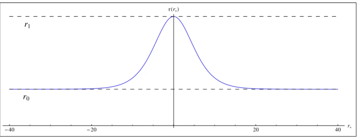
The form of (3.32) is illustrated in figure3.1. It is to be noted that (3.32) is monotonic increas-ing, implying that there are no additional horizons aside fromr1andr2. The function A(r∗),

with the result (3.32), is given by

A_(r_∗_{) =} 2κ1

r2−r1

(r2e−κ1r∗−r1e−κ1r∗) (r2eκ1r∗−r1eκ1r∗)

(e−κ1r_∗₊_eκ1r_∗₎2 +

O₍_δ3₎_, (3.33)

which can be simplified to

A_(r_∗_{) =} (r2−r1)κ1

2 sech

2₍_κ

(42)

3.3.2 Near extremal wormholes

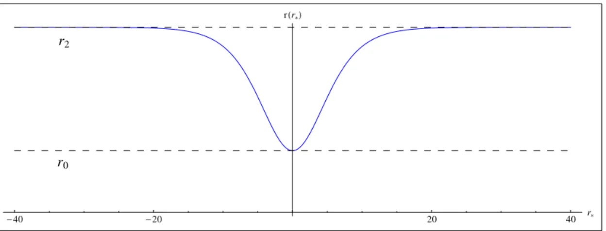
A second case of interest which admits a near extremal limit are the geometries introduced in [32] asnear extremal wormholes. Wormholes are compact spacetimes with non trivial

topolog-ical interiors and topologtopolog-ically simple boundaries, which can be seen as connections between otherwise distant or disconnected parts of the universe [33]. Near extremal wormholes typically appear in spacetimes with a positive cosmological constant, analogous to the near extremal Schwarzschild-de Sitter, and can be interpreted as limits of static and spherically symmetric solutions in world brane scenarios [32].

In the coordinate system(t,r,θ,φ)the near extremal limit of this spacetimes is given by

A(r) =A˜0(r2−r), (3.35)

B(r) =B˜0(r2−r)(r−r0), (3.36)

where ˜A0 and ˜B0 are positive constants which are defined explicitly in [32]. The coordinate system(t,r,θ,φ)is only valid in the regionr0<r<r2, wherer2is a Killing horizon assuming the role of a cosmological horizon. We define again a dimensionless parameterδ in terms ofr2 andr0

δ = r2−r0

r0 , (3.37)

we have that the surface gravity atr=r2is given by

κ =1

2

q

˜

A0B˜0(r2−r0) =1₂

q

˜

A0B˜0r0δ1/2. (3.38)

The near-extremal limit is obtained whenr0→r2, that is, 0<δ ≪1, and the surface gravityκ atr2approaches zero. Now we extend the coordinate system in the regionr0<r<r2by means of the tortoise coordinate(t,r_∗,θ,φ), solving the following integral

r_∗(r) =p_˜1

A0B˜0

Z _dr

(r2−r)p(r−r0)

. (3.39)

The solution of this integral is (based on [34])

r_∗(r) =p_˜ 1

A0B˜0(r2−r0) ln

√

r2−r0−√r−r0 √

r2−r0+√r−r0

, (3.40)

which can be reformulated as

r_∗(r) = 1

2κln

(r2−r0)−(r−r0)

r₋r0+ (r2−r0) +2√r2−r0√r−r0

Perturbações em torno de buracos negros e seus duais algébricos

UNIVERSIDADE DE SÃO PAULO

INSTITUTO DE FÍSICA