The Role of Income Inequality on Fiscal Multipliers
Bruno D. Q. Franco
∗January 7, 2015
Nova School of Business & Economics
University of Maastricht
Master Thesis developed under the advisory of Professors Francesco Franco and Tom van Veen.
Abstract
This paper investigates the role of income inequality on the size of fiscal multipliers during the recent crisis. Using various measures of income inequality, the empirical strategy developed suggests a positive and statistically significant impact of inequality on the size of fiscal multipliers of European economies during 2010-11. The results are robust after controlling for the role of outliers, by adding controls that could be driving the results, testing for different forecast vintages, and using a different source of standardized income inequality data.
Theoretical arguments that may explain the results are presented. Namely the existence of credit constraints to relatively poor households, and the lower propensity to consume of relatively wealthier households.
Keywords: Fiscal policy, forecasting, income inequality, government expenditure, output fluc-tuations.
∗Double Degree Student of Economics at Nova School of Business & Economics and University of Maastricht. Student
1
Introduction
After the 2008 crisis, a significant number of advanced economies were forced to undertake measures
of fiscal consolidation. The high levels of government debt were the main driving force for such necessity.
However, the short-term effects of those government spending cuts or tax hikes on economic activity
(the so-calledfiscal multipliers) were highly uncertain.
A large body of literature has been devoted to study the size of the fiscal multiplier, using
dif-ferent techniques for the fiscal policy identification. Seminal contributions include Blanchard and
Perotti (2002), Mountford and Uhlig (2009), and Ramey (2011). However, different model classes,
identification strategies, and specifications yield far from consensual results.1
More recently, the literature on fiscal multipliers has evolved to allow for state-dependent
multi-pliers, thus rejecting the hypothesis of a permanent, time-invariant multiplier. In fact, the economic
context during the crisis was particularly complex. This, in turn, added to the uncertainty surrounding
the consequences of fiscal consolidation measures. For that contributed the binding zero lower bound
on nominal interest rates, the presence of increased financial frictions, and a greater deal of slack in
the economy, with a greater degree of underutilized resources.
In an influential paper published by the International Monetary Fund (IMF), Blanchard and Leigh
(2013) conclude that real GDP growth forecast errors for 26 European economies were systematically
correlated with fiscal consolidation forecasts during the recent crisis. Specifically, countries with higher
levels of fiscal consolidation forecasts registered, on average, more negative growth forecast errors.
These results imply that professional forecasters systematically underestimated the impact of fiscal
consolidation measures on growth, and suggest multipliers well above 1 earlier in the crisis. Robustness
tests were performed and their baseline results still hold after the control of outliers, the inclusion of
additional variables that are likely correlated with both growth forecast errors and fiscal consolidation
forecasts, and for different forecast vintages.
The main goal of this paper is to investigate the relation between income inequality and the size
of the fiscal multiplier. The methodology follows closely Blanchard and Leigh (2013) by
interpret-ing growth forecast errors as higher-than-normal fiscal multipliers. Such a framework suggests that
higher-than-expected fiscal multipliers caused higher growth forecast errors during 2010-11. Using the
European Union Statistics on Income and Living Conditions (EU-SILC) dataset, we construct various
measures of income inequality for the same 26 European economies.
The empirical strategy used suggests that the countries with higher pre-crisis levels of income
inequality registered, on average, higher growth forecast errors during their fiscal consolidation efforts
for the period 2010-11. According to the framework developed, these results provide evidence of
larger-than-expected multipliers. The obtained coefficients have relevant sizes and are statistically
significant. We also test for a non-linear relation between income inequality and the fiscal multiplier.
The results suggest that income inequality has a higher marginal impact on fiscal multipliers for
higher inequality levels. The baseline results are robust after controlling for the influence of outlier
observations, after adding controls that could cause higher-than-expected growth downfalls and be
related with our regressors, after checking that the relation does not hold for more normal times
(1997-2008), and using a different source of standardized income inequality.
Our estimation results also suggest that the relation between income inequality and the fiscal
mul-tiplier depends on the income definition used to measure inequality. Specifically, the results provide
evidence that the distribution of income among European economies only affected the fiscal
multi-plier in 2010-11 if measured by household disposable income. The relation does not seem to hold if
one accounts for the market (rather than disposable) distribution of income, where market income is
calculated gross of income taxes and social security employee contributions. These results have very
in-teresting implications by suggesting that European governments’ redistributive policies actually ended
up increasing the impact of fiscal policy on real growth.
In section 2 theoretical insights are presented regarding the relation between income inequality and
the size of fiscal multipliers. Specifically, it is possible that countries with higher levels of inequality
had a higher share of liquidity constrained households, and/or a higher share of agents with a higher
marginal propensity to consume. As long as there is a mapping between income inequality and any of
these channels, it is possible that income inequality may affect how contractionary fiscal consolidation
policies are. This section also provides a brief literature review on state-dependent fiscal multipliers.
Thus, complementary to Blanchard and Leigh (2013) findings, our results suggest that forecasters
did not underestimate the impact on growth of fiscal consolidationper se. Instead, they suggest that
forecasters underestimated the consequences of heterogeneity of agents during fiscal austerity.
The remainder of this paper is organized as follows. Section 3 includes an overview of Blanchard
and Leigh’s (2013) work, and describes the empirical procedure developed to test if income inequality
had an impact on fiscal multipliers during 2010-11. The section finalizes with additional testing on
various dimensions: by using different economies and controlling for the impact of possible outliers, by
including additional controls, by assessing whether the relationship holds for more normal times
(1997-2008), and using a different source of standardized income inequality data. Section 5 shows evidence
regarding liquidity constrained households for some euro area countries during 2010, and relates with
the measures of inequality used in our baseline estimation results. The final section concludes.
2
Theoretical Background
Fiscal multipliers are defined as the effect that a fiscal shock (either positive or negative) has on
output. It represents the percentage change in real GDP (or real GDP growth) that follows a fiscal
shock totaling 1 percent of GDP. Despite playing a central role in fiscal policy analysis, there remains
an enormous range of views on its characteristics, namely its size.
Recent literature suggests that fiscal multipliers depend on economies’ circumstances as well as
underlying economic structures and policy regimes (beyond any variation related to the specific fiscal
measure at hand) (Corsetti et al., 2012). Spilimbergo et al. (2009) list a number of conditions
under which multipliers in general (and fiscal multipliers in particular) are larger. Specifically, fiscal
multipliers are larger if a) the fiscal consolidation impacts especially on consumption (rather than on
savings) or mainly reduces the consumption of domestically produced goods (rather than imported
ones), and b) the monetary conditions cannot adapt to offset the negative short-term effects of fiscal
consolidation (e.g., interest rates cannot decrease due to a binding zero lower bound on nominal interest
rates).
An additional circumstance prone to influence the size of the fiscal multiplier, but with the opposite
effect, is the state of public finances. Fiscal multipliers are generally assumed to be lower when
consol-idation is implemented during a rapid deterioration in public finances given the increased credibility
and confidence in sovereign health. The reduction in fiscal multipliers can be achieved through lower
sovereign spreads required by the market.2
The way income is distributed within an economy can, in turn, affect most of the aforementioned
conditions. Specifically, countries with a more unequal distribution of income (i.e., higher income
inequality) will have a higher share of lower income households. Consequently, this group of households
2Consumers’ expectations towards lower future taxation may also increase consumption in the short-run, thus
is likely to have a higher marginal propensity to consumevis-à-vis higher income households.3
In the
context of fiscal consolidation, this factor increases the size of the fiscal multiplier. The reason is that
a higher proportion of agents experience a reduction in their disposable income that was otherwise
targeted to consumption. Thus, the fiscal consolidation episode becomes more contractionary.
Dynan et al. (2004) consistently find that higher-lifetime income households save a larger fraction
of their income than lower-income households using three different sources of micro-data. This result
suggests that the rich do consume a smaller proportion of their income than the poor. Jappelli et al.
(2014) also find a substantial heterogeneity of marginal propensities to consume across income groups.
The authors use the 2010 Italian Survey of Household Income and Wealth and ask consumers how
much of an unexpected transitory income change they would consume. They find that the average
marginal propensity to consume declines sharply with cash-on-hand,4
from around 65 percent in the
lowest cash-on-hand percentile to 30 percent for the richest households.
Additional evidence is provided by Mian et al. (2013) for the U.S. economy after the housing
collapse of 2006 to 2009. They find that after a housing net worth shock, the marginal propensity to
consume varies significantly with income and debt levels. As the authors mention, the results suggest
that the aggregate impact of wealth shocks depends not only on the total wealth lost but also on how
these losses are distributed across the population.
Countries with higher income inequality are also prone to have a higher share of liquidity constrained
households. By having a higher share of lower income agents, it is likely that a higher proportion of
the households either do not possess enough wealth to resort during a negative income shock, or do
not possess enough collateral to borrow from financial institutions (Furman and Stiglitz, 1998). Thus,
during a fiscal consolidation episode, the negative income shock will force liquidity constrained families
to reduce their consumption levels, given their inability to borrow funds and smooth their consumption
path.5
Coenen et al. (2012) find a multiplier between 1 and 1.5 in various policy models that include
liquidity constrained households if monetary policy remains accommodative for 2 years. These results
are roughly twice as large as under normal conditions. Galí et al. (2007) extend the standard new
Keynesian model to allow for the presence of liquidity constrained households. The addition of this
3Differences in the marginal propensity to consume can arise for a number of reasons. Modigliani (1986) suggests
that life-cycle motives are the source of differences in saving behavior across households. Other economists have focused on the role of time preferences, characterizing a class of agents as “impatient” (Iacoviello, 2005, and Eggertsson and Krugman, 2010).
4Cash-on-hand is defined as the sum of household disposable income and financial wealth, net of consumer debt. 5The inability to smooth consumption may also occur if households’ wealth is held in illiquid assets, together with
non-Ricardian element to the model increases the sensitivity of current consumption to current
in-come levels. Thus, the authors find a larger fiscal multiplier in the presence of liquidity constrained
households.
Using a panel of nineteen OECD countries from 1970-2002, Tagkalakis (2008) also finds that fiscal
policy impacts more on consumption during economic recessions. The author purposes that liquidity
constraints are the driving force behind the asymmetric effects of fiscal policy on consumption over
the business cycle.
To the extent that income inequality affects either of the aforementioned channels, income
distribu-tion may affect the size of the multiplier. Furthermore, the economic situation in Europe early in the
crisis was particularly complex, increasing the uncertainty regarding the impact of fiscal consolidation
measures. One particular element to be considered was the binding zero lower bound on nominal
interest rates that rendered the European Central Bank with no (conventional) monetary policy.
Evi-dence from Christiano et al. (2011) show that, using a dynamic stochastic general equilibrium (DSGE)
model, an economy in a liquidity trap can have multipliers above 3. Further evidence is provided by
Woodford (2011) using a new Keynesian DSGE model. The author found that, in the presence of a
zero lower bound,6
multipliers can rise well above 1.
Thus, not only the economic context in general was prone to higher-than-normal multipliers, but
also countries faced different levels of income inequality. Then, it becomes important to investigate
whether those differences in income inequality, in the context of fiscal consolidation, played any role
on the size of the fiscal multiplier.
3
Inequality and Growth Forecast Errors
In this section, we present our model, explain the estimation procedure, describe the inequality
measures used, and present our results. To do that, we start by presenting Blanchard and Leigh’s
(2013) model and their results. After that, we focus on a model that explicitly includes income
inequality as a regressor, and present our baseline estimation results while exploring different relations
between income inequality and the fiscal multiplier.
3.1
Model Specification and Data
Our work investigates whether countries with higher levels of income inequality before the crisis,
6In fact, as mentioned in Woodford (2011), it only matters that the policy rate be at a level that the central bank
jointly with fiscal consolidation measures, had higher-than-forecasted real GDP growth
disappoint-ments. We interpret growth forecast errors as higher-than-expected fiscal multipliers.
In order to study these relations empirically, we start by presenting the parsimonious model
devel-oped in Blanchard and Leigh (2013). We decompose the model in question in order to fully comprehend
its meaning. Furthermore, when performing empirical analysis, this will make coefficient interpretation
clearer, thus allowing us to better understand what the data describes.
The model tries to capture the essence of the forecasting models used by forecasters. It starts by
assuming that real GDP growth can be expressed as the following equation:
4Yi,t:t+1 =mi,t:t+1·Forecast of4Fi,t:t+1|t+δi,t:t+1·Xi,t−2|t +ui,t:t+1, (1)
where∆Yi,t:t+1denotes cumulative (year-over-year) growth of real GDP in economyi -i.e., (Yi,t+1/Yi,t−1 1).
∆Fi,t:t+1|t denotes the change in the general government structural fiscal balance in percent of
poten-tial GDP, and is used as a measure of discretionary fiscal policy.7
Positive values of∆Fi,t:t+1|tindicate
fiscal consolidation, and negative values indicate fiscal stimulus. The resulting forecast is defined as
f{Fi,t+1 Fi,t−1|Ωt}, where f denotes the forecast conditional onΩt, the information set available early
in yeart. Xi,t−2|trepresents other exogenous variables that could affect the real GDP growth during
periodt to t+1, such as government debt, structural fiscal balance, etc.8
It is assumed that fiscal
consolidation forecasts during periodt to t+1 affect real growth through the fiscal multipliermi,t:t+1,
and the exogenous controls affect it viaδi,t:t+1. The last term,ui,t:t+1, is considered to be a zero mean
random disturbance.
If forecasters assumed an economy represented by the model in equation (1) to perform their
forecasts, their forecast in periodt can be represented as the expected value of that equation, given
the information available until that moment,Ωt,
Et[4Yi,t:t+1|Ωt] =mi,tˆ :t+1·Forecast of4Fi,t:t+1|t+δi,tˆ :t+1·Xi,t−2|t, (2)
wheremi,tˆ :t+1 and ˆδi,t:t+1 are the estimated multipliers. Thus, by computing the difference between
the observed and the forecasted real GDP growth,4Yobs
i,t:t+1 Et[4Yi,t:t+1|Ωt], Blanchard and Leigh
7As explained in the World Economic Outlook data appendix, “The structural budget balance refers to the general
government cyclically adjusted balance adjusted for nonstructural elements beyond the economic cycle. These include temporary financial sector and asset price movements as well as one-off, or temporary, revenue or expenditure items. The cyclically adjusted balance is the fiscal balance adjusted for the effects of the economic cycle; see, for example, Fedelino et al. (2009).
(2013) obtain the forecast error of real GDP growth. That is,
Forecast Error of∆Yi,t:t+1 = mi,t:t+1·Forecast of4Fi,t:t+1|t+δi,t:t+1·Xi,t−2|t+ui,t:t+1
( ˆmi,t:t+1·Forecast of 4Fi,t:t+1|t+δi,tˆ :t+1·Xi,t−2|t). (3)
Rearranging the terms in (3) shows that the forecast error of real GDP growth can be represented
as the difference between the actual multipliers and the estimated ones, plus a random disturbance,
Forecast Error of∆Yi,t:t+1 = (mi,t:t+1 mi,tˆ :t+1)·Forecast of4Fi,t:t+1|t
+(δi,t:t+1 δi,tˆ :t+1)·Xi,t−2|t+ui,t:t+1. (4)
Thus, aiming to investigate whether European countries registered higher-than-expected
multipli-ers during the beginning of the crisis, Blanchard and Leigh (2013) test if forecastmultipli-ers systematically
misspecified the impact of fiscal consolidation forecasts and other additional controls impacts’ on real
growth. They interpret systematic forecast errors made by professional forecasters as an indicator of
higher- or lower-than-expected multipliers. The authors propose the following empirical strategy:
Forecast Error of∆Yi,t:t+1=α+β Forecast of4Fi,t:t+1|t+γ Xi,t−2|t +εi,t:t+1. (5)
This equation relates growth forecast errors with fiscal consolidation forecasts and other lagged
controls, plus a random disturbance. The coefficients of fiscal consolidation forecasts and other controls
indicate the average growth forecast error associated with each additional unit of fiscal consolidation
forecasts and other lagged controls, respectively. The β andγ coefficients allow to investigate, for a
given period of time, if countries with higher levels of fiscal consolidation forecasts or other controls,
respectively, were systematically related with positive or negative growth forecast errors
In order to test the above relationship in the beginning of the crisis, growth forecast errors are
calculated for the period 2010-11 as the difference between actual cumulative real GDP
(year-over-year) growth, based on the latest (October 2014 WEO) data, minus the forecast prepared early in the
crisis (April 2010 WEO). The forecast of the change in the structural fiscal balance as a percentage
using all European Union’s 27 member states, plus Iceland, Norway, and Switzerland. However, since
WEO forecasts of the structural fiscal balance are not available for Estonia, Latvia, Lithuania, and
Luxembourg, the sample only includes the remaining 26 European economies.9
If the model was correctly specified and assuming rational expectations, estimation of equation (5)
should yield coefficients not statistically different from zero of fiscal consolidation forecasts and other
lagged controls. The zero coefficients would indicate that forecasters did not consistently over- or
underestimated the value of their forecast during the period 2010-11, which suggest forecast efficiency.
On the other hand, if the obtained coefficients were higher or lower than zero, this would suggest
that forecasters systematically over- or underestimated the contractionary effect of the regressors
in-cluded, respectively. This, in turn, would suggest that forecasters did not efficiently incorporate past
information into their information set (Nordhaus, 1987).
In fact, Blanchard and Leigh (2013) did find statistically significant estimates of β around 1.2
during 2010-11, and no significant estimates ofγ irrespectively of the control used.10
Thus, according
to equation (4), the results provided evidence that the real impact of each additional percentage point
of GDP of fiscal consolidation forecasts on real growth,4Yi,t:t+1, was underestimated by forecasters,
on average, by 1.2points. I.e., the actual fiscal multiplier of the 26 European economies included in
the sample during the early years of the crisis,m2010−11, can be expressed as the sum of the estimated
multiplier,mˆ2010−11, and the average underestimation,
m2010−11= ˆm2010−11+ 1.2. (6)
One should notice that the actual values of the fiscal multiplier, m2010−11 (as well as the ones
estimated by forecasters,mˆ2010−11), cannot be obtained with the framework developed above. In order
to calculate the value ofm2010−11, one needs to obtain a measure of a fiscal shock that is uncorrelated
with other economic developments. This ensures that the estimated coefficient reflects solely the
causal effect of the fiscal policy on growth, and not the response of growth on fiscal policy (through, for
example, automatic stabilizers). In the multipliers literature, this is called the identification problem of
9The 26 European economies included are Austria, Belgium, Bulgaria, Cyprus, Czech Republic, Denmark, Finland,
France, Germany, Greece, Hungary, Ireland, Iceland, Italy, Malta, Netherlands, Norway, Poland, Portugal, Romania, Slovak Republic, Slovenia, Spain, Sweden, Switzerland, and the United Kingdom.
10In fact, the work of Blanchard and Leigh (2013) reports an estimate ofβof
−1.095(t-statistic =−4.29) when no
additional controls are included (i.e., excludingXi,t−2|tfrom (5), since all of these yield non-significant coefficients, and
fiscal policy. The framework does, however, provide evidence of systematic miscalculation of forecasted
fiscal multipliers versus actual multipliers.
As mentioned, the authors investigated the possibility of having other variables - plausibly related
to fiscal consolidation forecasts and lower-than-expected growth - driving the results. The omission of
such variables could bias the analysis toward finding that multipliers were larger than assumed. The
variables in question are the countries’ debt ratio, their fiscal balance, their current account balance,
etc.11
However, given that the authors were interested in the causal effect of each of those variables
on growth forecast errors, and the variables are most likely endogenous in the above specification, the
authors included lagged (i.e., pre-crisis) values in equation (5). Nevertheless, none of the variables
in-cluded produced a statistically significant coefficient, nor they virtually changed the fiscal consolidation
estimation results.
There is, however, a group of controls that could potentially affect the growth forecast errors
that was not considered by Blanchard and Leigh (2013) - measures of income distribution among the
European economies. As mentioned in section 2, there are various channels through which countries
with higher levels of income heterogeneity can have higher multipliers. Specifically, given the multiyear
fiscal consolidation plans undertaken in 2010, it is possible that countries with higher levels of income
inequality registered higher growth forecast errors (in absolute terms) due to its impact on the fiscal
multiplier.
Thus, we now investigate if, in fact, income inequality affected the size of the fiscal multiplier of
European countries during the beginning of the crisis.
3.2
The Role of Inequality on Fiscal Multipliers
We start by describing the income inequality measures used, and then we present the estimation results
of a model that explicitly accounts for income inequality.
3.2.1 Income Inequality Measures and Data
We use the European Union Statistics on Income and Living Conditions (EU-SILC) data in order
to compute various measures of income inequality for the baseline results.12
This dataset contains
11The complete list of variables included as controls by Blanchard and Leigh (2013) is: pre-crisis (2009) debt ratio,
fiscal balance, structural fiscal balance, sovereign CDS, bank CDS, and a dummy for banking crisis as in Laeven and Valencia (2012). Additionally, the authors included the pre-crisis (2009) initial growth forecast, potential growth forecast, and for the 2007 current account balance, net foreign liabilities, household debt, and trading partners fiscal consolidation. 12We only use the EU-SILC dataset in this section because of unavailability of comparable data from other sources,
comparative statistics on income distribution in the European Union, collected via a harmonized
framework among the various member states. This ensures the comparability of inequality measures
across countries. The EU-SILC is also the most complete dataset available for European economies
for the economies and years studied.
In order to have a clear picture about the income distribution, and tackle the inherently difficult
task of measuring inequality, we create diverse measures of income inequality using EU-SILC dataset.
Namely we construct the Quartile ratio (share of top quartile to the first quartile), Quintile ratio, Decile
ratio, 5thPercentile ratio, Palma ratio13
, and the Gini coefficient of equivalised disposable income.14
The various measures of income inequality aim to provide a better description of the income
dis-tribution among the European countries analyzed. Listings 1 and 2 provide the lists of inequality
measures used for years 2008 and 2009, respectively. It also includes the values of other variables used
in the estimation of the baseline results.
3.2.2 The Model With Income Inequality
In order to investigate if inequality affected the size of the fiscal multiplier, we turn to the model
specified in subsection 3.1, and change the specification of the fiscal multiplier to be related with
inequality. After the fiscal multiplier being specified, we modify equation (5) in order to have a
framework that allows us to obtain testable hypothesis about the role of inequality on fiscal multipliers.
We start by specifying a fiscal multiplier, mi,t:t+1, linearly related to inequality. For concreteness,
consider
mi,t:t+1=νi,t:t+1+ρi,t:t+1Income Inequalityi,t−2|t, (7)
where bothνi,t:t+1andρi,t:t+1are constants. This specification for the fiscal multiplier implies that
fis-across countries. Additionally, the dataset only includes 11 inequality observations for the year 2008, and 5 observations for the year 2009 for the sample of countries we are analyzing. Similarly, the Luxembourg Income Study Database (LIS), despite using a harmonized framework that ensures cross country comparability of inequality measures, is only available for a very limited number of economies and years. We do, however, perform a robustness test in section 4 using the Standardized World Income Inequality Database.
13The Palma ratio, named after the work of the economist Gabriel Palma (2011), consists of the ratio of the top
decile to the four bottom deciles. This measures was created after Palma’s observation that while the deciles 5 to 9 (the “middle class”) tend to capture about 50% of national income on a cross countries basis, the other half of national income varies considerably across countries between the richest 10% (top decile) and the poorest 40% (four bottom deciles).
14Unless otherwise specified, Gini measures always refer to the Gini coefficient of equivalised disposable income (i.e.,
obtained using after taxes and transfers data).
cal policy affects real growth through an autonomous component,νi,t:t+1, plus a component dependent
on the income inequality level,ρi,t:t+1. Using this specification, we change equation (4) accordingly to
obtain:15
Forecast Error of ∆Yi,t:t+1 = (ν νˆ)·Forecast of4Fi,t:t+1|t+ (δ δˆ)·Income Inequalityi,t−2|t
+(ρ ρˆ)·Forecast of4Fi,t:t+1|t·Income Inequalityi,t−2|t
+εi,t:t+1. (8)
Note that the fiscal multiplier is assumed to be related with pre-crisis levels of income inequality,
rather than contemporaneous levels. The reason is that income inequality is most likely an endogenous
variable in equation (8). On the one hand, higher income inequality can be theresult of
lower-than-expected growth via, for example, lower redistributive policies. On the other hand, higher income
inequality can be the cause of lower growth through, for example, one of the channels previously
mentioned, such as a higher share of liquidity constrained households. Thus, we follow Blanchard and
Leigh (2013) and deal with this potential endogeneity by lagging the variables. Specifically, we use
both 2008 and 2009 as pre-crisis years of income inequality.16
In order to test whether income inequality had any effect on the size of fiscal multipliers during the
crisis, and following the spirit of the empirical model presented on (5), we perform the following OLS
regression:
Forecast Error of ∆Yi,t:t+1 = α+β Forecast of∆Fi,t:t+1|t +γ Income Inequalityi,t−2|t
+η Forecast of∆Fi,t:t+1|t ·Income Inequalityi,t−2|t
+υi,t:t+1. (9)
This model consists of the estimation of equation (5) using pre-crisis income inequality as a
con-trol, augmented with the interaction between fiscal consolidation and lagged income inequality. The
resulting estimates of β can be interpreted as the average forecast error caused by each additional
15The included controls,X
i,t−2|t, are pre-crisis levels of income inequality. Also, the indexes onνandρare suppressed
in order to make the equations more easily readable.
16In practice, using both 2008 and 2009 for pre-crisis years of inequality translates into using income inequality for
percentage point of GDP of fiscal consolidationwhenIncome Inequalityi,t−2|tis zero. This coefficient
is not very illustrative since episodes of perfect income equality are very atypical.
On the other hand,γ is an estimate of the average forecast error caused by each additional point
of pre-crisis inequalitywhen Forecast of ∆Fi,t:t+1|tis zero. 17
This coefficient allows to investigate if
countries with higher levels of income inequality registered higher-than-expected multipliers during
2010-11 other than through the fiscal multiplier.
Finally, estimates of η measure the average forecast error caused by each additional point of
pre-crisis income inequalityand fiscal consolidation. This is the most interesting coefficient in our
speci-fication since it allows us to test whether countries with higher inequality had, in fact, higher growth
downfalls during their fiscal austerity plans. Negative values of η provide evidence that forecasters
underestimated the impact of inequality on fiscal multipliers.
Given the specification of the fiscal multiplier in equation (7), we can write an expression for the
(average) true fiscal multiplier as:
m2010−11= (νˆ2010−11 β)+ (ρˆ2010−11 η)·Income Inequalityi,t−2|t. (10)
The multiplier can thus be expressed as the sum of the forecasted components, minus their average
estimation “error”. Specifically, the true fiscal multiplier during 2010-11 can be expressed as the sum of
two components: the forecast of the autonomous component of the fiscal multiplier,νˆ2010−11, minus the
β coefficient estimated in equation (9), and the estimated inequality-dependent component,ρˆ2010−11,
minus the estimatedη coefficient, adjusted for the country-specific level of inequality.
Recall that, according to equation (7), we are assuming a fiscal multiplier that depends on income
inequality. I.e., we are assuming that the impact of fiscal policy on real growth may be affected by the
level of income inequality. Thus, the above equation is an extension of equation (6) that separates the
effects that influence the size of the fiscal multiplier into two components. One component,(ˆν2010−11
β), captures the impact of fiscal policy on real growth that does not depend on inequality (i.e., when
income inequality is equal to zero). The other component,(ˆρ2010−11 η), captures the impact of fiscal
17In order to understand this point, one should take the partial derivative of Forecast Error of∆Y
i,t:t+1with respect
to Forecast of∆Fi,t:t+1|tand Income Inequalityi,t−2|t, respectively. Since the partial effect of the Forecast of∆Fi,t:t+1|t
on the Forecast Error of∆Yi,t:t+1(while holding income inequality constant) is given by
∂E(Forecast Error of∆Yi,t:t+1)
∂Forecast of∆Fi,t:t+1|t =β+ηIncome Inequalityi,t−2|t,
the value ofβ can be interpreted as the partial effect of fiscal consolidation on the Forecast Error of∆Yi,t:t+1 when
Income Inequalityi,t−2|t is zero. The same reasoning applies to the partial effect of income inequality on the Forecast
policy on real growth that is dependent on income inequality. Consequently, since this component is
assumed to depend on inequality, we need to adjust for the country-specific level of inequality. Hence,
we multiply it for the level of inequality.
3.3
Baseline Results
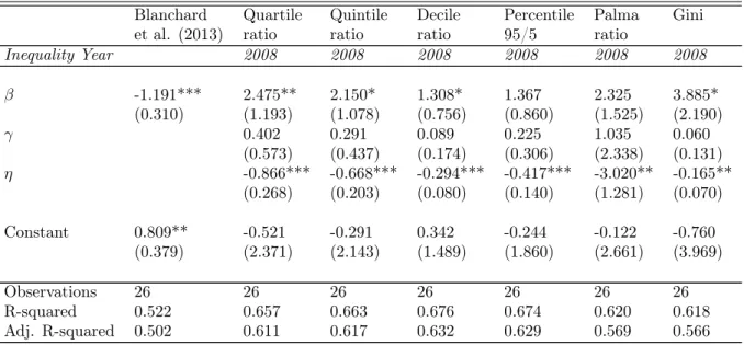
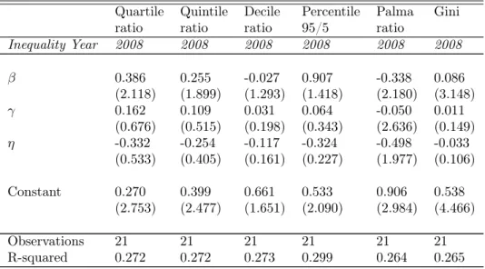
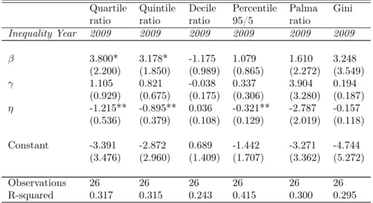
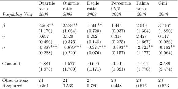
The OLS estimation results for the period 2010-11 are presented in Tables 1 and 2.18
Our empirical
model suggests a statistically significant negative relation between the interaction term (Forecast of
∆Fi,t:t+1|t·Income Inequalityi,t−2|t) and growth forecast errors. The results hold for various measures
of income inequality, with the interaction coefficient varying considerably in size, depending on the
inequality measure used. Regarding statistical significance, the results obtained are highly significant
for most inequality measures used for the pre-crisis year 2008, with mostp-values below 1 percent.
However, before proceeding, it is important to review the meaning of thet-statistics and resulting
p-values of the interaction term. Contrary to the coefficients obtained with Forecast of ∆Fi,t:t+1|tand
Income Inequalityi,t−2|tindividually, one cannot infer about its statistical relevance using its individual
significance. Because income inequality enters the model via an interaction term, its marginal effect on
growth forecast errors are conditional on the fiscal consolidation forecasts. As a result, the marginal
effect of income inequality on growth forecast errors can be significant for substantially relevant values
of fiscal consolidation forecast, even if the coefficient on the interaction term is insignificant.19
Thus,
in order to infer about the relevance of including the interaction term in the model, one should first
calculate the standard error of the marginal impact of income inequality on growth forecast errors.
Alternatively, one could also plot the marginal effect of inequality on growth forecast errors for different
values of fiscal consolidation forecast. This way, it is possible to visually check if the estimated
confidence intervals are above or below zero at any region of the graph. If they are, that provides
evidence that under such values of fiscal consolidation, the marginal impact of inequality on growth
forecast errors is statistically significant at the given confidence level.
As mentioned, the coefficients vary considerably in size, depending on the inequality measure used.
The highest values of the interaction coefficient are obtained using the Palma Ratio, with a coefficient
of 3.020 and 3.282 for the pre-crisis years of 2008 and 2009, respectively. The lowest values of
18Throughout the paper, all forecast errors are computed relative to the latest (October 2014 WEO) dataset. Also,
the reported statistical inference is based on heteroskedasticity-robust standard errors. All the confidence intervals are calculated using the conventional 95% confidence level.
19For a deeper discussion about the interpretation of interaction terms on econometric models, see Brambor et al.
interaction are obtained with the Gini coefficient for the year 2008 (with an estimate of 0.165), and
with the Decile ratio for the year 2009 (estimate of 0.087).
The estimated coefficients of Income Inequalityi,t−2|t, γ, are not significantly different from zero.
These results hold for all the measures of income inequality included, and for both pre-crisis years. As
explained before, the zero coefficient of pre-crisis income inequality on growth forecast errors provides
evidence that its impact on growthwhen there are no fiscal policywas not misspecified. I.e., excluding
the impact via the fiscal multiplier, pre-crisis income inequality does not impact on growth beyond
forecasted.
The coefficients of Forecast of ∆Fi,t:t+1|t display positive but mostly insignificant results. The
statistical significance is dependent on the inequality measure used, and it varies from the 2008 to the
2009 specification. One must, however, recall that this coefficient measures the average forecast error
caused by each additional percentage point of GDP of fiscal consolidationwhenIncome Inequalityi,t−2|t
is zero. Thus, given that episodes of complete absence of income inequality are logically irrelevant, we
find this coefficient very little informative.
Since the marginal impact of income inequality on fiscal multipliers varies with the amount of fiscal
consolidation, we use a graph to depict how much that impact changes for different values of fiscal
consolidation forecasts. Figures 1 and 2 present the marginal effect of pre-crisis income inequality using
both pre-crisis years (2008 and 2009), where the dashed lines represent the 95% confidence interval.
From the graphs it is possible to assert that the marginal impact of pre-crisis income inequality increases
(in absolute terms) the forecast error of real growth the higher the fiscal consolidation measures.
Thus, higher levels of fiscal consolidation are associated with more negative growth forecast errors via
the impact of higher income inequality. According to the framework developed above, this provides
evidence that pre-crisis income inequality increased the size of the fiscal multiplier during 2010-11.
Complementary to Blanchard and Leigh’s (2013) conclusions, by obtaining simultaneously a
neg-ative estimate of the interaction term and a zero coefficient of income inequality, our results suggest
that forecasters did not underestimate the impact on growth of fiscal consolidationper se. Instead,
they suggest that forecasters underestimated the consequences of heterogeneity of agents during
fis-cal austerity. In conclusion, the obtained results provide evidence that, in fact, the distribution of
income within each European country played an important role on how contractionary were the fiscal
consolidation measures during the recent crisis.
inequality - is taken into account, the source of misspecification becomes clearer. Economies with more
heterogeneous agents suffered higher growth forecast errors during their fiscal consolidation efforts.
This, according to our specification, provides evidence of higher fiscal multipliers as a result of income
inequality.
3.4
Is the Relation Between Inequality and Fiscal Multipliers Linear?
We now turn to the specific relation between income inequality and the fiscal multiplier. Until now we
have assumed a linear relation between inequality and the multiplier. This was clear by the specification
presented on equation (7). But is the marginal impact of inequality on the size of the multiplier really
constant (as a result of a linear relationship), or does the marginal impact of income inequality on the
multiplier increase/decrease with the amount of inequality?
In order to test this hypothesis, we start by defining a multiplier related to inequality in a non-linear
fashion, specifically in a quadratic form:
mi,t:t+1=νi,t:t+1+ρi,t:t+1Income Inequalityi,t−2|t +σi,t:t+1Income Inequality 2
i,t−2|t. (11)
whereνi,t:t+1,ρi,t:t+1, andσi,t:t+1are constants. This particular specification relates fiscal policy with
real growth via an autonomous component, a component dependent on inequality, and a newly added
component dependent on squared inequality, aiming to capture its non-linear behavior.
After modifying equation (4) to include this multiplier specification, and still using lagged inequality
as a control, it is possible to empirically test this model according to the following framework:
Forecast Error of ∆Yi,t:t+1 = α+β Forecast of∆Fi,t:t+1|t +γ Income Inequalityi,t−2|t
+η Forecast of∆Fi,t:t+1|t ·Income Inequalityi,t−2|t
+κForecast of∆Fi,t:t+1|t·Income Inequality
2
i,t−2|t
+υi,t:t+1. (12)
The additional interaction term with squared inequality aims to capture decreasing or increasing
zero suggest the existence of non-linear forces between inequality and its impact on the size of the
fiscal multiplier. Specifically, negative values of theκcoefficient indicate that forecasters, on average,
underestimated more than proportionally the impact of higher levels of income inequality on growth
forecast errors. This, in turn, suggests that the marginal effect of income inequality on the size of the
fiscal multiplier increases with the level of inequality. The opposite goes for positive values of theκ
coefficient.
Given this specification, we present how to calculate the marginal impact of income inequality:
∂E(Forecast Error of∆Yi,t:t+1)
∂Income Inequalityi,t−2|t
= γ+η Forecast of∆Fi,t:t+1|t
+2κForecast of∆Fi,t:t+1|t ·Income Inequalityi,t−2|t. (13)
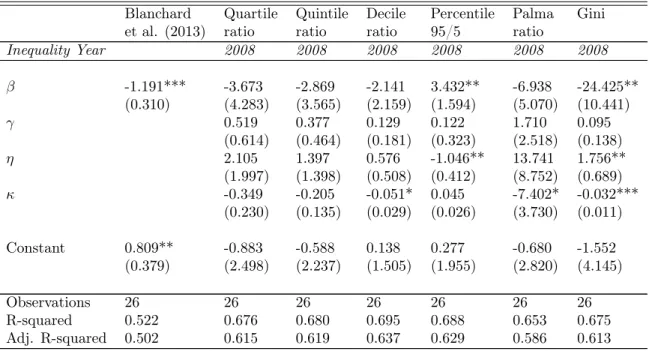
The results of the OLS estimation of equation (12) are presented in Tables 3 and 4. The coefficient
that includes the squared inequality, κ, has a negative sign for the majority of income inequality
measures used. The negative sign provides evidence that income inequality causes marginally
higher-than-expected growth downfalls for higher levels of income inequality. The results, however, display
different levels of statistical significance, depending on the income inequality measure used and, mostly,
on the pre-crisis year of inequality. Nevertheless, recall that one cannot infer about the relevance of
the interaction terms simply by looking at the significance of the coefficients on the interaction terms.
Since, according to our specification, the marginal effect of income inequality on growth forecast
errors - and, thus, on the fiscal multiplier - is dependent upon the levels of income inequality itself and
fiscal consolidation, we present a three-dimensional graph to analyze the obtained results. Figures 3
and 4 present the graphs for the different measures of income inequality and for both pre-crisis years.20
As the graphs depict, higher levels of income inequality jointly with higher levels of fiscal
con-solidation forecasts increase the size of the marginal impact of inequality on growth forecast errors.
The marginal impact of income inequality varies considerably with the inequality measure used. The
results are robust to most income inequality measures used,21
and for both pre-crisis years of income
inequality. In conclusion, these results provide evidence that an increase of one unit of pre-crisis income
20The graphs are constructed to display the marginal effect of income inequality on the growth forecast error according
to reasonable values of fiscal consolidation forecast and income inequality. Those reasonable values are constrained
between the maximum and minimum values of both fiscal consolidation forecasts and income inequality among the 26 European economies studied, and for the years analyzed.
21The exception being the 5th Percentile ratio and Decile ratio for the pre-crisis years 2008 and 2009, respectively.
inequality had a stronger marginal impact on the size of fiscal multipliers the higher the initial value
of income inequality.
But which of the models considered (linear versus non-linear) explains better the data? The
R-squared does not answer this question since the linear model of equation (9) is nested on the non-linear
model of equation (12). This implies that the R-squared of the non-linear model will be necessarily
higher than the R-squared obtained with model (9) given the extra regression term. This way, we look
at the Adjusted R-squared, which penalizes the extra number of regressors, to compare both models.
The Adjusted R-squared between the linear and non-linear models are not very different for both
pre-crisis years of income inequality. Even though it is higher for non-linear models using most income
inequality specifications, the difference cannot be considered very significant. These results, in turn,
suggest that the non-linear component of income inequality adds little information explaining the data.
4
Robustness Tests
We now determine the validity of the obtained results by performing some robustness tests. The
results reported by Blanchard and Leigh (2013) suggest that countries with larger planned fiscal
con-solidation had, on average, larger growth disappointments during 2010-11. These results hold after a)
controlling for different groups of economies and limiting the influence of potential outlier observations,
and b) adding control variables to the equation that could plausibly have both affected the growth
forecast error and been correlated with fiscal consolidation. The authors also find that the relation
does not hold for forecasts made in more normal times (1997-2008), as one would expect.
In our baseline specification developed on subsection 3.2, the results show that countries with
higher levels of pre-crisis income inequality in the context of fiscal consolidation reported, on average,
higher real GDP growth declines during the crisis. This is, according to the framework presented,
evidence that inequality increased the size of the fiscal multiplier during 2010-11. Thus, in order to
determine the validity of our results, we now perform some robustness checks. Specifically, we perform
the same tests as in Blanchard and Leigh (2013), plus an additional test with a different source of
income inequality measures.22
22Ideally, one extra robustness test would be performed - estimation of equation (9) with wealth and consumption
4.1
Using Di
ff
erent Economies and Their Sensitivity to Outliers
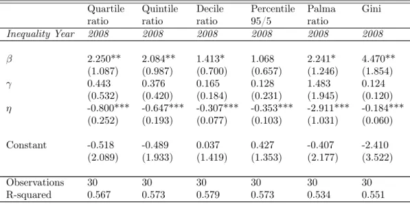
We start by investigating whether the obtained results change if the countries included in the sample
also change. As mentioned earlier, the WEO dataset did not have available forecasts for the structural
fiscal balance available of four EU member states - Estonia, Latvia, Lithuania, and Luxembourg. Thus
we first re-estimate our results replacing those four missing observations with European Commission
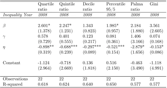
forecasts. The results are presented in Tables 5 and 6.
The estimated coefficients are virtually unchanged, and yield the same conclusions as the baseline
model specified in equation (9). More specifically, the interaction term between pre-crisis income
inequality and fiscal consolidation forecasts is still negative, irrespectively of the income inequality
measure used, and the coefficient of income inequality on growth forecast errors is still statistically
non different from zero. These results provide additional evidence that income inequality affected
growth forecast errors through its impact on the fiscal multiplier.
Then, we test the sensitivity of the results to countries with the largest interaction (in absolute
terms) of fiscal policy change forecast and income inequality. The two countries with the highest
abso-lute values of both fiscal policy change and income inequality are Germany and Greece, irrespectively
of the inequality measure used and the pre-crisis year (2008 or 2009).23
The results are presented in
Tables 7 and 8. As expected, the obtained coefficients of interaction decrease in size. However, the
obtained results still conserve the negative sign of interaction, and the zero coefficient of income
in-equality when there are no fiscal consolidation forecasts. The income inin-equality measure that yield the
highest impact on growth forecast errors (in absolute terms) is still the Palma ratio, with an interaction
coefficient of 1.764 and 1.908 for the pre-crisis years of 2008 and 2009, respectively. The lowest
interaction coefficients are obtained with the Gini measure of inequality. Its estimated coefficients are
0.094 for 2008 and 0.090 for 2009.
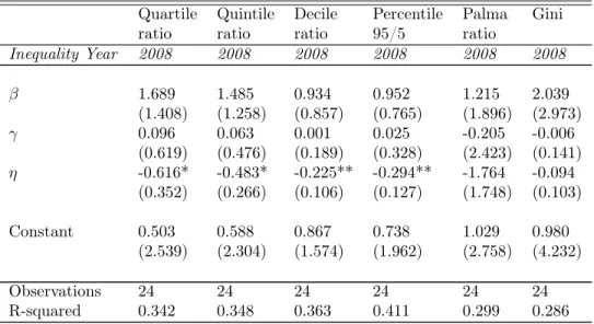
As an additional test, we check the sensitivity of the results by excluding the economies under
IMF assistance programs during 2010-11. Given the nature of IMF assistance programs to lend money
to countries in severe financial trouble, it is likely that those countries had a relatively high fiscal
consolidation forecasts and, perhaps, high levels of income inequality. The countries in question are
Portugal, Greece, Ireland, Iceland, and Romania. In fact, this group of countries registered relatively
higher levels of both fiscal consolidation forecasts and inequality in the beginning of the crisis.
23Denmark is an exception by standing as the country with a higher interaction of forecast of fiscal policy change
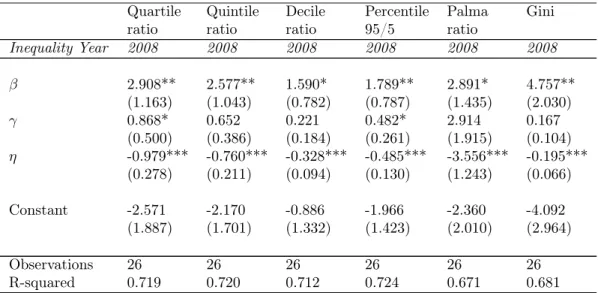
The resulting OLS estimations are presented in Tables 9 and 10. The results hold for all 2008
measures of income inequality, with a negative estimated interaction coefficient, and a zero coefficient
for income inequality individually. However, the estimated coefficients produce positive interaction
coefficients when we include 2009 measures of income inequality. These results suggest that income
inequality levels in European economies (excluding the ones under IMF assistance programs during
2010-11) changed from 2008 to 2009 in a way that rendered its relationship with fiscal multipliers less
clear.
We also re-estimate our results excluding from the sample the four economies classified as “emerging”
in the WEO database. Those economies are Bulgaria, Hungary, Poland, and Romania. See Tables 11
and 12 for the results. Once again, our baseline results are robust to the exclusion of the four emerging
economies of our dataset.
Next, we apply different estimation strategies constructed to resist the influence of potential outliers.
The first method employed is a robust regression, which down-weights observations with larger absolute
residuals using iterative least squares. By down-weighting influential outliers, this estimation procedure
is less influenced by them than ordinary least squares (OLS) estimations. The estimated coefficients
are presented in Tables 13 and 14. We can assert that our baseline conclusions were not being driven by
outliers, given that the estimated coefficients are very similar to the ones estimated using OLS. Then,
the same exercise is performed but using a quantile regression approach. This estimation procedure
minimizes the sum of the absolute residuals about the median, rather than about the mean as in OLS.
This makes the estimates less affected by outliers. The estimation results are presented in Tables 15
and 16. The results still hold using this estimation procedure, with more sizable coefficients being
obtained with pre-crisis year 2008.
As a last robustness check,24
we re-estimate our results using Cook’s distance method. Specifically,
we re-estimate our results deleting observations with a Cook’s distance greater than 4/N, whereN is
the sample size. The results are presented in Tables 17 and 18, and, once again, show that our baseline
results were not being driven by the influence of outliers.
24Given that there are no harmonized inequality data collected for the additional 10 advanced economies listed in
4.2
Controlling for Other Variables
We now test the robustness of our results in a different dimension. Specifically, we test if the obtained
results were being driven by some other factors that could plausibly have affected both the interaction
of inequality with fiscal consolidation and lower-than-expected growth.
In order to test for this, we extend our model developed in subsection 3.2 to include an additional
control variable. This way, if the obtained results still hold after the inclusion of these additional
variables that could possibly affect the interaction of inequality with fiscal consolidation and
lower-than-expected growth, we have evidence that those additional factors were not driving the results.
The control variables included in our specification are all pre-crisis levels (2008 and 2009). The
reason is that we are interested to know if forecasters underestimated the causal effect of some factors
- other than the interaction of inequality with fiscal consolidation forecasts - on growth. However, if
we include those variables during 2010-11 in our estimations, the coefficients obtained do not measure
such causal effect since the variables suffer from endogeneity - i.e., they can simultaneously be the
causeand theresult of lower-than-expected growth. Thus, in order to obtain the causal effect of those
controls on growth, we use pre-crisis values. This way, we ensure that the estimation only captures
the causal effect of controls on growth.
In order to ensure that the variables were included in the forecasters’ information set, we use
the same dataset as the fiscal consolidation forecasts - the April 2010 WEO. We start by including
backward-looking measures of fiscal accounts, such as the pre-crisis government-debt-to-GDP ratio,
pre-crisis fiscal-balance-to-GDP ratio, and the pre-crisis structural fiscal-balance-to-GDP ratio. The
results (not shown) are virtually unchanged when those fiscal measures are included as controls. The
results hold for pre-crisis years 2008 and 2009 of both inequality and controls. The results are also
robust when we include the average five-year sovereign credit default swap (CDS) spread in the first
quarter of 2009 and 2010.
Next, we check whether larger-than-expected financial sector stress are driving the results. Thus
we control for pre-crisis bank CDS spread, and for a dummy variable indicating a systemic banking
crisis, as identified by Laeven and Valencia (2012). The results remain unchanged, thus providing
evidence that financial sector developments were not driving the baseline results.
Lastly, we also control for the trade-weighted fiscal consolidation of other countries (scaled by the
share of exports in GDP, given that fiscal consolidation by trading partner countries may be driving the
in percentage of GDP, and the household-debt-to-disposable-income-ratio. The results to all these
robustness checks suggest that our baseline estimations were not being biased by the exclusion of these
control variables.
4.3
Using Di
ff
erent Forecast Vintages
The work developed until now focused on forecasts produced in early 2010, when a number of large
fiscal consolidation plans were announced. However, as mentioned in Blanchard and Leigh (2013), it
is worth analyzing whether the results also hold for forecasts made in other years. Specifically, it is
important to test if the results hold for forecasts produced in more normal times (1997-2008). Thus
we now investigate whether the interaction term of lagged income inequality and fiscal consolidation
forecasts still has a negative impact on growth forecast errors using forecasts made in more normal
times. As stated before, forecast efficiency requires forecast errors not to be systematically related to
any of the regressors. So, our expectation is that the interaction term coefficient should be around
zero for these different forecast vintages.
The empirical strategy now consists in including a set of two-year intervals during the pre-crisis
decade (1997-2008) together in a panel. We follow Blanchard and Leigh (2013) and write the equation
as:
Forecast Error of ∆Yi,t:t+1 = α+λt+β Forecast of ∆Fi,t:t+1|t+γ Income Inequalityi,t−2|t
+η Forecast of∆Fi,t:t+1|t·Income Inequalityi,t−2|t
+υi,t:t+1. (14)
This equation is simply our equation (9) augmented with a vector of time-fixed effects,λt, wheret
= 1997, 1998, ..., and 2008. Since we are using two-year overlapping intervals, we use the Newey-West
procedure to correct for MA(1) serial correlation. Once again, the exercise is performed for various
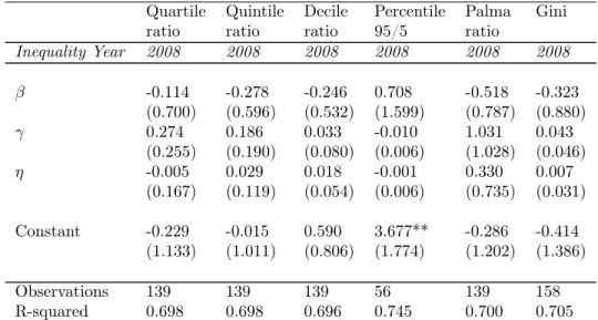
measures of income inequality, and the estimation now includes 139 observations for most income
inequality specifications. Recall that we are using lagged income inequality in order to ensure that
causality runs from inequality to growth forecast errors.
The estimations results are presented in Table 19. As we expected, the coefficient of the interaction
hold for the various measures of income inequality included in the sample, with coefficients varying
from 0.005 using the Quartile ratio to 0.330 using the Palma ratio.
On the one hand, these results suggest that, in fact, during normal times, forecasters did use the
correct model specification in their forecasts. As a result, growth forecast errors were not systematically
related with the interaction of lagged income inequality and fiscal consolidation forecasts during the
pre-crisis decade. One the other hand, given the systematic and consistent growth forecast errors made
by forecasters in the beginning of the crisis (2010-11), this test provides an extra robustness check
that, in fact, the uncertainty regarding the size of the fiscal multipliers was exceptionally high during
that period. As a result, forecasters systematically underestimated the impact of fiscal consolidation
measures on real growth. According to our particular framework, the results suggest that one of the
channels through which fiscal consolidation measures impacted on growth was via the distribution of
income.
4.4
Using a Di
ff
erent Source of Income Inequality Data
We also test the robustness of our results using a different inequality dataset. Specifically, we use
data from the Standardized World Income Inequality Database (SWIID) for the same 26 European
economies. Even though this dataset relies solely on Gini measures of income inequality, it maximizes
the comparability of available data for the broadest possible sample of countries and years (Solt, 2009).
Interestingly, this dataset introduces two different Gini measures - one calculated using household
dis-posable income (similarly to the one we used with the EU-SILC dataset), and another using household
market income (i.e., pre-tax and pre-transfer).
Thus we re-estimate equation (9), but this time using inequality data from the SWIID dataset.
The resulting estimation output is presented in Table 20 for both 2008 and 2009 inequality measures.
The graphs depicting the marginal impact of income inequality on growth forecast errors are presented
in Figures 5 and 6.
The estimated results showed in the first and third columns in Table 20 display a negative relation
between the interaction term and growth forecast errors. These results are obtained with an
interac-tion term composed by the pre-crisis disposable income Gini and fiscal consolidainterac-tion forecasts. The
results hold for both 2008 and 2009 pre-crisis years of income inequality. Additionally, the estimated
coefficients are very similar to the ones estimated with the Gini using EU-SILC dataset. Specifically,
respec-tively. Recall that the results obtained for the Gini coefficient using the EU-SILC dataset (that are also
calculated using disposable income data) are 0.165 and 0.173 for 2008 and 2009, respectively. The
similarity between the magnitude of the estimated coefficients is reassuring and gives more confidence
to the results obtained.
Also, and similarly to the baseline results, the coefficient of income inequality individually is also
not statistically significant for both pre-crisis years of income inequality. Thus, the baseline results are
entirely robust to the use of this harmonized dataset.
Figures 5 and 6 also indicate that the relation between the interaction term and growth forecast
errors breaks down when income inequality is measured by market (rather than disposable) income.
Despite displaying a slightly negative marginal impact of inequality on growth forecast errors for both
pre-crisis years, this impact is not statistically significant. From the figures, it is possible to see that the
estimated coefficients are not significant independently of the amount of fiscal consolidation forecast.
More formal evidence is also presented in the second and fourth columns of Table 20.
In order to better understand the meaning of these results, one needs first to understand how
the Gini (pre-tax and pre-transfer) measures are constructed. According to the Luxembourg Income
Study (LIS) Harmonization Guidelines,25
the market income Gini is constructed using amounts gross
of income taxes and social security employee contributions (but not employer contributions). By
sub-tracting the overall amount of taxes and contributions to the gross income, one obtains the household
disposable income.
On the one hand, our results suggest that themarket distribution of income of European economies
did not affect the fiscal multiplier during 2010-11. That is, the distribution of income accrued to
households before government’s intervention in the market (through income taxes and social security
employee contributions) did not have a mapping with the fiscal multiplier early in the crisis. On
the other hand, according to our baseline results and various robustness tests, the way income was
distributed after government’s intervention (i.e., the distribution of householddisposable income) did
affect the fiscal multiplier. Specifically, European countries with higher levels of household disposable
income inequality registered, on average, higher fiscal multipliers during 2010-11.
This is a very important result. It provides evidence that government’s redistributive policies
25The LIS Harmonization Guidelines are available at
http://www.lisdatacenter.org/wp-content/uploads/our-lis-documentation-harmonisation-guidelines.pdf.
altered the distribution of income in a manner that increased the fiscal multipliers during 2010-11.
I.e., it suggests that fiscal policy itself changed the distribution of income in a way that its impact on
the real economy (i.e., the fiscal multiplier) increased. Thus, according to our results, it is not the
way income is distributed by the market that affected the size of the fiscal multiplier. It is the way
government’s redistribute income that actually increased the fiscal multiplier early in the crisis.
5
Extension
So far we have presented evidence that, early in the crisis, European economies with higher
pre-crisis levels of income inequality registered higher-than-expected growth downfalls during their fiscal
consolidation plans. We interpreted those results as higher levels of income inequality causing
higher-than-expected fiscal multipliers. However, we were intentionally silent about the possible channels
through which income inequality may materialize into higher fiscal multipliers.
In section 2 we presented some possible channels through which that relation may occur. Those
channels included a higher share of households among more unequal countries with a higher marginal
propensity to consume and/or with a binding liquidity constraint. In this section, we briefly present
some data from the Eurosystem Household Finance and Consumption Survey (HFCS). This dataset
contains information about households’ assets and liabilities, income, and indicators of consumption
and credit constraints for 15 euro area countries. The HFCS survey reports their results having 2010
as base year.
From the microdata available, we constructed the proportion of liquidity constrained households
for each country. Following Martin et al. (2014), we defined a liquidity constrained household as
one with liquid assets below two months of its total gross income. These measures were created for
different subgroups of the population. Specifically, we created the proportion of liquidity constrained
households among indebted households, and the total fraction of liquidity constrained in the economy
(i.e., that includes both indebted and not indebted households). The type of debt considered can result
from mortgages and consumer credit.
In order to investigate if, in fact, countries with higher levels of income inequality registered a higher
proportion of liquidity constrained households, we plot various graphs between the two variables. More
specifically, we are interested to know if european countries with higher levels of income inequality
measured during 2008 and 2009 faced a higher proportion of liquidity constrained households during
both variables depends on the definition of liquidity constraints. I.e., if the results vary when using
liquidity constraints restricted to indebted households versus the total fraction of liquidity constrained
households.
Figures 7 and 8 present the graphs relating the proportion of indebted households that face a
liquidity constraint and income inequality. In order to ensure consistency, we plotted the proportion
of indebted liquidity constrained households in 2010 and the various income inequality measures used
in the baseline results for both 2008 and 2009. Additionally, we also included the R-squared obtained
for each linear regression.
A first look at both figures does not seem to suggest a very strong relation between the percentage
of indebted liquidity constrained households and the different measures of income inequality.
Conse-quently, measures of income inequality may not be a good proxy for the share of liquidity constrained
households. However, there is a couple of countries that seem to appear as outliers in this analysis:
Slovenia and Slovak Republic. One possible explanation for the exceptionally high share of liquidity
constrained households in these countries may be their relatively lower financial development.
Hence the fitted line presented, and thus the estimated R-squared, excludes those two countries
from the regression. As Figures 7 and 8 show, there is a positive relationship between the income
inequality level and the proportion of liquidity constrained households among those that are indebted.
The obtained R-squared of around 0.25, nevertheless, suggests that there is a large fraction of liquidity
constraints variation among european economies that is not explained by income inequality. However,
one also needs to take into account the low sample of countries included (only 13 countries given that
we have excluded Slovenia and Slovak Republic).
When the same exercise is performed using the total share of liquidity constrained households
(instead of restricting the sample to indebted agents), the above relationship does not seem to hold.
However, these results (not showed) are not surprising given our definition of liquidity constraints.
Recall that we consider that a household is liquidity constrained if its liquid assets are below two
months of its total gross income. Nevertheless, in practice, a liquidity constraint is binding when
agents cannot borrow as much as they would optimally do. So, despite a household with liquid assets
below two months of its total gross income being considered liquidity constrained in our specification,
it does not mean that in practice the agent will not be able to borrow funds. Thus, it is much more
plausible that agents that already hold debt will face, on average, much more restrictive borrowing