doi: 10.1590/0101-7438.2015.035.03.0489
LAGRANGE MULTIPLIERS IN THE PROBABILITY DISTRIBUTIONS ELICITATION PROBLEM:
AN APPLICATION TO THE 2013 FIFA CONFEDERATIONS CUP
Diogo de Carvalho Bezerra
1*and Leandro Chaves Rˆego
2Received February 15, 2014 / Accepted June 19, 2015
ABSTRACT. Contributions from the sensitivity analysis of the parameters of the linear programming model for the elicitation of experts’ beliefs are presented. The process allows for the calibration of the family of probability distributions obtained in the elicitation process. An experiment to obtain the proba-bility distribution of a future event (Brazil vs. Spain soccer game in the 2013 FIFA Confederations Cup final game) was conducted. The proposed sensitivity analysis step may help to reduce the vagueness of the information given by the expert.
Keywords: Elicitation, linear programming, soccer and sensitivity analysis.
1 INTRODUCTION
“It is notable that the probability that emerged so suddenly is Janus-faced. On the one side it is statistical, concerning itself with stochastic laws of chance processes. On the other side it is epistemological, dedicated to assessing reasonable degrees of belief in propositions quite devoid of statistical background.”
Ian Hacking (1975)
The purpose of a knowledge (or belief) elicitation process is to obtain one or more probability distributions that represent the experts’ beliefs in a random event,π(θ ). A parameterized dis-tribution is usually assumed to facilitate the elicitation process. A method of elicitation of the experts’ knowledge based on linear programming is proposed in Nadler Lins & Campello de Souza (2001) and Campello de Souza (2002). In Nadler Lins & Campello de Souza (2001), em-phasis is given to the dificulty indicators of the elicitation process for the random variable case. Campello de Souza (2002) generalizes the model for the case without a random variable.
*Corresponding author.
The contribution of Lagrange multipliers analysis to the model proposed by Campello de Souza (2002) is an unresolved problem and the main objective of this paper. A set of elicitations on the prediction for the Brazil vs Spain soccer match in the 2013 Confederations Cup is conducted; in terms of probabilistic predictions, the method proposed should be seen as one more option. In general, if the objective was to make a prediction of that particular game, the applied method should be used along with other methods, in the same way that other variables on the outcome of soccer matches should be taken into account. In any case, a presentation of the references on Campello de Souza’s method (2002) and of the existing methods of soccer predictions, as well as the differences and similarities involved is necessary.
Ferreira et al. (2009) states that among the elements of the decision problems there is the knowl-edge gained by the experts through a priori probability distributions, the model presented by Nadler Lins & Campello de Souza (2001) being one of the options to obtain the a priori distribu-tion. Studies by Nadler Lins & Campello de Souza (2001), Silva & Campello de Souza (2005) and Bezerra & Campello de Souza (2011) are applications of elicitation methods of inaccurate probabilities through linear programming in decision problems in medicine in the first two cases, and selection of portfolio in the third one. The application of Campello de Souza’s method for elicitation of prior distributions in the Brazil vs Spain soccer is just an illustration. Thus, the ap-plication is not the main contribution of this article. A general review of elicitation methods, as well as of the model presented in Nadler Lins & Campello de Souza (2001) and its relationship with other methods is presented in Burgman et al. (2006).
Several methods developed in operational research (Data Envelopment Analysis – DEA, Ordinal Methods, Logit Model, Preference Probabilistic Composition) are found in the literature, as well as principles (Home advantage and weak rationality) are used in soccer issues such as: rules for resource distribution, alternative rankings, home advantage evaluation, performance evalua-tion, identification of unexpected results. Studies by Sant’Anna (2008), Sant’Anna et al. (2010), Alves et al. (2011a, b), Sant’Anna and Mello (2012) are examples of the application of such methods in Brazilian and South-American soccer championships.
Among the advantages of the method proposed by Campello de Souza (2002), the fact that it is compatible with other views of probabilistic representation as well as the possibility to answer other soccer questions, such as the question of the alternative ranking, can be highlighted. It is evident that changes in the elicitation questionnaire will be necessary in this case. Studies by Campello de Souza (1983) and Campello de Souza (1986) are classical references regarding the probabilistic preferences with triangle inequalities in order to obtain inaccurate and imprecise preferences, which have been recently proposed in the analysis of conflict stability (Santos & Rˆego, 2014; Rˆego & Santos, 2015).
2 ELICITATION OF IMPRECISE PROBABILITIES VIA LINEAR PROGRAMMING In his book, Treatise on Probability (Keynes, 1979), Keynes supports the hypothesis that, in the long run, we will all be dead and that historical data which would allow making predictions about our future would never exist. Thus, when there is little data or no data, the expert’s a priori knowledge should be used.
A general model that can represent all aspects of random phenomena is still far from being achieved. The method for obtaining probability distribution families proposed by Campello de Souza (2002) and developed in Nadler Lins & Campello de Souza (2001) and Silva & Campello de Souza (2005) becomes an alternative. Burgman et al. (2006) classifies the proposed model in Campelo de Souza (2002), among the imprecise probability models (Walley, 1991).
The elicitation method of the expert’s a priori distribution has as basic assumption the fact that the expert has vague knowledge about the probability distribution of the random event of interest,
π(θ ). It is also assumed that it can make “only a finite number of comparative probabilistic assertions” when answering questions about the likelihood of a random variable to take a value in one of two ranges. The method leads to expressing the expert’s knowledge as families of probabilities distributions, featuring the human being’s natural limitations. Thus, the expert’s knowledge could be represented by a set of probability distributions limited by “a stochastically greater distribution than all other distributions compatible with the answers that have been given”, as well as by a stochastically distribution lower than all others.
Initially, an elicitation questionnaire is proposed. Considering the case where the state of nature,
θ, is a real and continuous parameter, the plausible range forθ should be established, in other words,[θmin, θmax), where the probability that the value ofθ is out of this range is zero. The range is partitioned into 2n subintervals. Then, πj = Pr(θ ∈ [θj−1, θj)) is defined, where
j =1, . . . ,2n−1.
In the method in question, there are three possible statements about the probability mass between two subintervals, ofθj, or possible combinations of subintervals:
First Statement – Comparison of Probabilities: given two subintervals,[θs, θt)and[θu, θv), wheret ≤u, the expert can compare their probability masses, in other words,A1is a set of statements of typeπs+1+πs+2+ · · · +πt ≤πu+1+πu+2+ · · · +πvorπs+1+πs+2+ · · · +πt ≥ πu+1+πu+2+ · · · +πv– (in the case where the expert cannot compare the given subintervals, the corresponding question is left blank).
Second Statement – Odds Ratios of Probability Masses: given two subintervals,[θs, θt)and [θu, θv), wheret ≤u, the expert can establish a lower or upper bound on the odds ratios between the two given intervals; in other words,A2is a set of statements of type
πs+1+πs+2+ · · · +πt πu+1+πu+2+ · · · +πv
≤a or πs+1+πs+2+ · · · +πt
πu+1+πu+2+ · · · +πv ≥a,
Third statement – Difference between Probability Masses: given two subintervals, [θs, θt)
and[θu, θv), where t ≤ u, the expert can establish a lower or upper bound on the dif-ference between the odds ratios of the two given intervals; in other words, A3 is a set of statements of type(πs+1+πs+2+ · · · +πt)−a(πu+1+πu+2+ · · · +πv) ≤ bor (πs+1+πs+2+ · · · +πt)−a(πu+1+πu+2+ · · · +πv)≥b, wherea>0 andb∈ ℜ.
The model consists of solving two linear programming problems, namely, first, solving a maxi-mization problem and, second, a minimaxi-mization one, subject to the same set of constraints obtained from the expert’s survey responses. Mathematically, they are expressed as follows:
max(min)πj 2n
j=1
cjπj (1)
subject to:
(−1)f(r)
⎛
⎝
k(r)
j=t(r) πj−ar
m(r)
j=l(r) πj
⎞
⎠≤br (2)
2n
j=1
πj =1 (3)
πj ≥0,j =1,2, . . . ,2n (4)
wherek(r) <l(r),ar >0,r =1, . . . ,q,q is the number of questions answered by the expert
and f(r)∈ {0,1}and its value depend on ther-th response to the expert’s questionnaire. Depending on the combination of parametersar andbr, the expert’s opinion can be captured in many ways. The two last restrictions are to ensure that one has a probability distribution. Coefficientscj may be placed as the sum of the area of cumulative probability distribution. In this
case, the goal would be to minimize the expected value when solving the maximization problem, and maximize the expected value when solving the minimization problem. This is made possible by consideringcj =2n− j+1. Using the fact thatθj =θ0+j a, wherea =θj−θj−1, it can be shown (Campello de Souza, 2002) that maximizing
2n
j=1
(2n− j+1)πj
is equivalent to minimizing
2n
j=1
θjπj.
optimization problem is empty, it means that the expert was not consistent in his responses. The questions not answered by the expert will not enter the constraints of the linear programming problem.
It is now possible to present the dual model and perform a sensitivity analysis of the elicitation model.
3 THE DUAL MODEL: LAGRANGE MULTIPLIER AND SENSITIVITY ANALYSIS
Another mathematical programming problem known as the dual problem can be set to any math-ematical programming problem with constraints (known as primal problem). The solution to both problems must be the same. The dual problem arises from the use of auxiliary variables, known as Lagrange multipliers, used to incorporate restrictions into the objective function of the problem. Considering the model presented in the previous section, the aim is to obtain the distributions
which provide the maximum and the minimum expected value by makingcj = 2n− j +1.
The choice of the objective function of the problem could be another one, but in this case, the problem can be considered a first order estimation; in other words, there is an attempt to esti-mate the mean of the distribution. However, other objective functions can be used, such as the variance or the entropy of the distribution. Any of these other functions would make the opti-mization problem nonlinear. Another way to incorporate the other quantities into the problem is for the researcher to use them in desired restrictions. Again, the problem would become nonlin-ear. The interpretation of the Lagrange multiplier in the dual problem depends on the choice of the objective function, the linear case being the one analyzed here.
3.1 The Simple Case
The behavior of the model is observed in a case with only two outcomes in which only a single question is answered by the expert. The model could then be written as follows:
max π1,π2
(min π1,π2
)E =c1π1+c2π2 (5)
subject to:
π1−aπ2≤b(or ≥b, depending on the response.) (6)
π1+π2=1 (7)
π1≥0 ,π2≥0 (8)
For the case of maximizing and minimizing the expected value, the values arec1=2 andc2=1. The dual problem can be written as
min λ1,λ2
(max λ1,λ2
)C=bλ1+λ2 (9)
subject to:
λ1+1λ2≥2 (10)
−aλ1+1λ2≥1 (11)
Studying the primal model for the case where b = 0, as there are only two constraints, this problem can be represented as in Figure 1. Considering the case where constraint (6) is of type ≤, since the slope of the objective function is equal to −2, the maximum is obtained at the point where constraint (6) is satisfied in equality, the values that maximize the objective function beingπ1 = a+11 andπ2 = a+a1. Thus, in this case, the value of the Lagrange multiplierλ1is positive. In the second case, where the problem is to minimize the expected value, the optimum is attained at π1 = 0 andπ2 = 1; consequently, λ1 = 0. The dashed line between points
(π1, π2)=
a a+1,
1
a+1
and(π1, π2)=(0,1)represents the feasible set.
When a Lagrange multiplier is zero to any question, the interpretation is that it does not con-tribute at all to obtaining the optimal distribution, being the answer to the corresponding question deductible from the other answers.
π1
π2
a a+1 1
a+1
1
1 feasible set
Figure 1–Simple Linear Programming Model.
3.2 An Interpretation for the Lagrange Multiplier
In Economics, linear programming models are typically used as tools for interpreting economic phenomena. This is a typical case where economic thinking produces scientific knowledge. In most cases, the analogy is made with physics or biology, but it can also be made with economic thinking. The objective function is what is desired. In the case of the firm, the objective function can be understood as the profit of a company, coefficientsar representing the coefficients of a
technological matrix, the value ofbr being the availability of an input, and the interpretation made of the Lagrange multiplier is that it reflects the opportunity cost, in terms of profit, of not having more of one of the inputs.
If b = 0, then coefficient a represents exactly the odds ratios between the two probabilistic masses and, in this case, the expert states no positive value for the difference between the odds ra-tios of the probabilistic masses. However, this does not mean that there is no opportunity cost re-lated to this question. If the inequality constraint becomes an equality constraint, in other words, in the example aboveπ2= 1aπ1, there will be an associated cost, since the expected value will not be higher in case of minimization, or will not be lower in case of maximization for not having a positive value, whichever it is, for the difference between the odds ratios of the probabilistic masses of the two given intervals. If the expert could refine this information by introducing a positive value for the difference between the odds ratios of the probabilistic masses, the model would provide a difference between the maximum and minimum expected values, smaller or equal, increasing the accuracy of his elicited beliefs.
Whenλ=0, this implies that the corresponding answer to the question is informative about the phenomenon and the question is considered active. If the number of active questions is big, it means that there is contribution of a large number of questions in the questionnaire to obtain the distributions.
3.3 The General Case
To favor the presentation of the general case of the dual problem, the inequality will always be considered as≤. Yet, it is easy to see that, regardless of the answer given by the expert, it is possible to transform the constraint into an inequality of this type. The linear programming problem described in (1)–(4) can be put in matrix form to make the presentation of the problem easier. Thus, wherec=(c1, . . . ,cj),πT =(π1, . . . , πj),bT = (b1, . . . ,bq),1 =(1, . . . ,1) and
A= ⎛
⎜ ⎜ ⎝
a11 . . . a1m ..
. . .. ... aq1 . . . aqm
⎞
⎟ ⎟ ⎠
, ai j = ⎧ ⎪ ⎨
⎪ ⎩
(−1)f(i), t(i)≤ j ≤(i);
ai(−1)f(i)+1, l(i)≤ j≤m(i);
0, c.c.
Therefore, the problem proposed in (Campello de Souza, 2002) can be rewritten with its respec-tive dual as follows:
Primal Dual
maxπj F =cπ subject to:
Aπ ≤b 1π=1
π ≥0
minλr,λs G=b
Tλ r+λs subject to:
ATλTr +λs≥cT
λr≥0 andλsFree
minπF =cπ subject to:
Aπ ≤b 1π =1
π≥0
maxλr,λsG=b
Tλ r+λs subject to:
ATλTr +λs ≥cT
λr≤0 andλsFree
3.4 Sensitivity Analysis
The sensitivity analysis of parameters consists of assessing the changes in the defined objective function of the problem, given an infinitesimal change in the values ofar orbr. This paper fol-lows the presentation in (Intriligator, 1971) in the use of the Langrangean function for sensitivity analysis. The Lagrangean function is defined at the optimum point as
L∗=cπ∗−λr∗(Aπ∗−b)−λ∗s(1π∗−1)
or
L∗= 2n
j=1
cjπ∗j − q
r=1
(−1)f(r)λr∗ k(r)
j=t(r) π∗j −ar
m(r)
j=l(r) π∗j −br
−λ∗s
2n
j=1
π∗j −1
.
Then the following proposition can be obtained:
Proposition 3.1.Given an optimal solution(π∗, λr∗, λ∗s)to the problem
maxπj F=cπ
subject to Aπ ≤b 1π=1
π ≥0, if λr=0 for some restriction r, then
∂L∗ ∂br ≥
∂L∗ ∂ar
Proof: Given that
L∗= 2n
j=1
cjπ∗j − q
r=1
(−1)f(r)λr∗ k(r)
j=t(r) π∗j −ar
m(r)
j=l(r) π∗j −br
−λ∗s
2n
j=1
π∗j −1
,
it follows that ∂∂La∗
r = (−1)
f(r)+1λ∗
r
m(r)
j=l(r)π ∗
j and ∂L∗
∂br = (−1)
f(r)λ∗
r. By restriction, we
have that 0≤m(r)
j=l(r)π ∗
j ≤1. Thus,
∂L∗ ∂br
= |λ∗r| ≥ |λ∗r|
m(r)
j=l(r) π∗j =
∂L∗ ∂ar .
The demonstration for the case of minimization is similar. The immediate consequence of the above proposition is that if the goal is to decrease the length of the interval between the minimum and maximum expected values of variableθ, where maxF = E(θ )and minF = E(θ ), then a marginal change inbr, i.e., in the group of the third statements, is more relevant than the same
4 APPLICATION: THE FIFA CONFEDERATIONS CUP 2013
The application of elicitation processes to sports is already well established in the literature Winkler (1971). There are two application examples of elicitation in worldwide soccer matches Walley (1991) and Andersen et al. (2007). In both cases, the methods of elicitation used bets in games to elicit the expert’s opinion. The former is an application for a specific game of the 1982 World Cup (Brazil×Russian) and in the latter the application is to find out whether Brazil would win the 2006 World Cup.
4.1 The Example of a Soccer Game
In Walley (2000), the author presents an example of statements about the possible outcomes of a soccer game to make comparisons between models of imprecise probability. In a soccer game, there are three possible outcomes: victory W, draw, D and defeat, L. Considering an expert making three qualitative judgments about the possible outcomes of the game:
⎧ ⎪ ⎨
⎪ ⎩
‘not winning’ is more likely than winning; winning is more likely than losing; a draw is more likely than losing the game,
To implement the elicitation method proposed by Campello de Souza (2002), it is necessary to define the objective function. Since a random variable which allows for the calculation of the expected value is not defined, some possibilities may be suggested. There are two types of soccer competitions: consecutive points championships, where the winning team is granted three points; a draw gives one point to each team; a defeat, zero to the team beaten. The second type of championship is known as cup or knockout stage confrontation in at least one of its phases and, in this case, only one team remains in the competition, making it a zero-sum game. In the former situation, the objective function can be written asX = 3IW +ID, which gives the number of points scored in a match, whereas in the latter, the objective function can be written as
X =3IW −3IL. The use of the function of the latter situation was chosen for the calculation of the distributions in the experiment. Thus, the linear programming model, according to the method proposed by Campello de Souza (2002), for the example by Walley (2000), can be written as follows:
max(min)(π(W),π(D),π(L))E(X)=3π(W)−3π(L) subject to
π(W)≤π(D)+π(L) π(W)≥π(L) π(D)≥π(L) π(W), π(D), π(L)≥0
As seen in Section 2,E(X)should be maximized as well as minimized in order to obtain the set of probability distributions. First, the experts’ statements must be made sure to be a nonempty set, proving to be consistent. Distributions that maximize (minimize) the expected value are shown in Table 1. Aspects on Lagrange multiplier’s behavior to model constraints were never observed. There are four restrictions to be observed, the first three are related to the expert’s qualitative judgment and the last is the equality constraint to obtain a probability distribution, the Lagrange multiplier being always active on this constraint since it is an equality constraint. For the first three statements, the maximization problem of Lagrange multipliers will be(1.5;0;0). With this result, only the first judgment is being used to determine the maximum E(X). In the minimization problem, the Lagrange multipliers are (0; −3;0); in this case, only the second judgment informs about the probability distribution that minimizesE(X).
Table 1–Lower and upper distribution – Soccer Game. max –π min –π
W 50.00% 25.00% D 50.00% 50.00% L 0.00% 25.00%
E(X) 1.5 0
4.2 The Choice of the Objective Function
Given the possibilities of the kind of competition, an interesting problem arises regarding the choice of the objective function. There are two alternative linear programming problems with respect to the representation of points in consecutive games: the first problem has already been described, considering the values of the points earned by the home team, X =3IW +ID; the
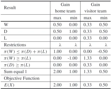
alternative problem is to consider the earnings by the visitor team Y = 3IL +ID. EventsW, DandL are always considered taking the home team in the point of view. Hence, if the home team loses(L), the visitor gets 3 points. As the method indicates minimizing and maximizing the objective function, the same set of probability distributions can be expected to be found, but this is not what happens. It can be said that, despite the fact that both models represent the same situation, the results are different and this problem of choice of the objective function can be considered as an example of the Framing Effect problem (Tversky & Kahneman, 1981). The results for both problems are presented in Table 2.
4.3 Study Design
Table 2–Framing Effect In the Elicitation of Soccer Game.
Result Gain Gain
home team visitor team max min max min
W 0.50 0.00 0.33 0.50
D 0.50 1.00 0.33 0.50
L 0.00 0.00 0.33 0.00
Restrictions λ λ λ λ
π(W)≤π(D)+π(L) 1.00 0.00 0.00 -0.50
π(W)≥π(L) 0.00 -1.00 1.33 0.00
π(D)≥π(L) 0.00 0.00 0.33 0.00
Sum equal 1 2.00 1.00 1.33 0.50 Objective Function
E(X) 2.00 1.00 0.33 0.50
into two phases, a confrontation between Brazil and Spain (World Champion) could already be anticipated to only occur in the finals.
Before the beginning of the 2013 FIFA Confederations Cup, an experiment with undergraduate students of Economics was held. Two groups of students were selected from a total of 23 stu-dents. The first group was characterized as experienced students in the course and, therefore, in probability and game theory, as they were undergraduate seniors. The second group were begin-ner students in the Economics course, who, despite their initial training in probability, did not have any complete training in Economics, as they were undergraduate sophomores. There were nine students in the first group, six men and three women. The second group had eight men and six women.
The experiment was divided into three parts, the questions being presented to the students fol-lowing the type of questions presented in Section 2. Firstly, students responded to probability statements of the first kind; later, of the second type and, finally, of the third kind. It was optional for the students not to answer any or all questions of a particular group. All questions referred to the possible match between Brazil and Spain. The first set of questions were about the following events:W,DandL, where each one represented Brazil’s victory, draw and defeat, respectively. Which one of the following events is more likely to occur:
1. W or (DandL)?
2. (W andD) orL? (The answer may define if the expert believes in the home advantage phenomena (Sant’Anna & Mello, 2012).)
The statements about the odds ratios and differences between probabilistic masses are related to the first five questions and formed the next two parts of the experiment. X = 3IW −3IL was used as the objective function in the linear programming problems. Three linear programming problems were analyzed. The first considered only the first group of statements; the second considered also the second set of statements; finally, the third linear programming problem con-sisted of all groups of statements. Five restrictions regarding the statements were presented in each problem, as well as the necessary condition for the probabilities to add up to one. The re-sponses to each set of statements of the five questions above by the 23 experts are shown in Table 4 in the Appendix. For instance, Expert 1’s answers to the first question in each group of statements are as follows: in the first group of statements, he considered Brazil’s defeat more likely than a draw or a victory; the value of the odds ratios of the probability masses, a1, was equal to 3 in the second group of statements for the same question and, finally, he considered the upper bound for the difference between the odds ratios of the probability masses,b1, equal to 0.1. The interpretation of the answers to the other questions and by the other experts, given in Table 4 in the Appendix, is similar.
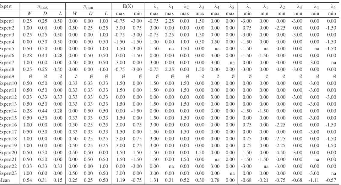
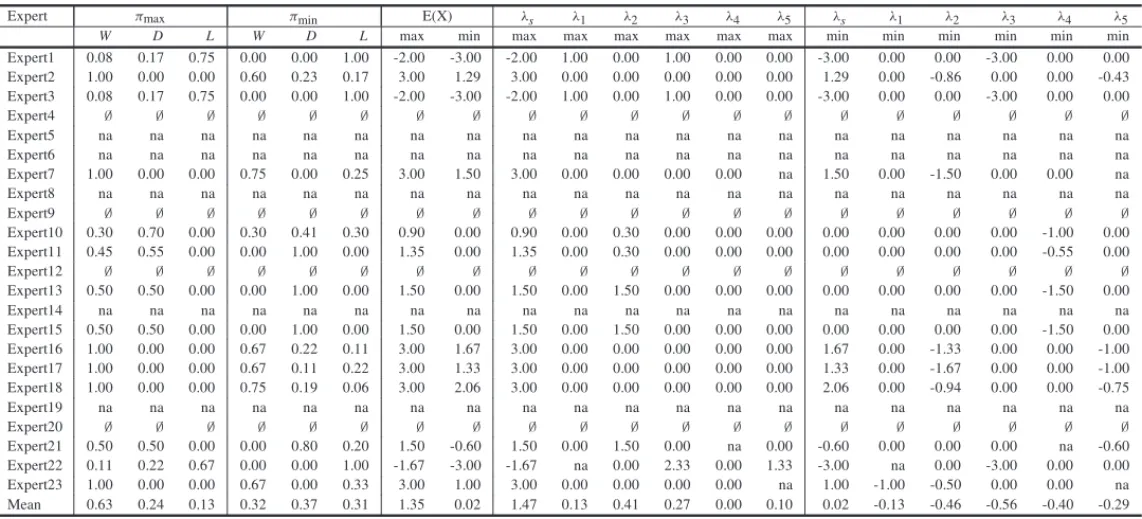
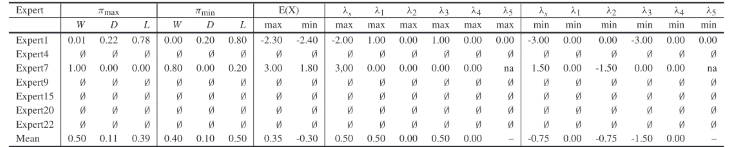
The results of the three linear programming problems are shown in Tables 5, 6 and 7 in the Appendix. As expected, as information is added to the linear programming problem, the length of the interval between the minimum and maximum expected values of points to be obtained seems to decrease. Taking the first expert as an example (one of the few who answered the three types of questions without generating any inconsistency), for the first set of information, the expected score was observed to be between [−0.75; −3.00], considering the odds ratios, the interval shrinks to[−2.00; −3.00]; finally, considering all the questions, the length of the interval gets even smaller[−2.30; −2.40]. Figures 2 and 3 show the distributions that maximize and minimize the expected points in a match by experts 1 and 14, respectively.
Another point to highlight is that the elicitation method shows experts’ inconscistencies regarding their probabilistic knowledge. Knowledge about football is inherent to most Brazilians, but this does not necessarly mean a bias in favor of Brazil’s victory when eliciting Brazilian experts, since at least 9 out of 23 experts had decided for Brazil’s defeat in the fourth question.
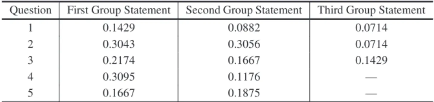
Finally, a question information index is proposed. When the Lagrange Multiplier of a question is active, there is an indication that this question is limiting the growth of expected values and, consequently, the question tells something about the expert’s opinion. Given the experiment with the 23 experts, the proposed index reflects which of the five questions were relevant to the experts elicited family of probability distributions. The information index is defined as:
Iλx =
L
2N (13)
whereLis the number of times the multiplier is nonzero, considering the maximization and min-imization problem, and N is the number of experts who answered questionx. The information index for each question per group of statements is shown in Table 3.
state-(X)
1
X
−3 0 3
0.75
0.50
Maximum Expected Value (solid) Minimum Expected Value (dashed)
Figure 2–Family of Probability Distributions of Expert 1.
(X)
1
X
−3 0 3
0.28 0.72
0.50
Maximum Expected Value (solid) Minimum Expected Value (dashed)
Figure 3–Family of Probability Distributions of Expert 14.
Table 3–Information Index for Each Question by Group of Statements. Question First Group Statement Second Group Statement Third Group Statement
1 0.1429 0.0882 0.0714
2 0.3043 0.3056 0.0714
3 0.2174 0.1667 0.1429
4 0.3095 0.1176 —
ments. On the other hand, the information index of the second question was more stable consid-ering the first and second groups, being above 0.3 in both groups. Thus, if one must choose a single question for the first two groups of statements, question 2 should be chosen.
5 CONCLUSION
The main contribution of this paper is to propose a sensitivity analysis evaluation of the linear programming problem used to obtain families of probability distributions arising from experts’ answers to a questionnaire, enabling a refinement of their knowledge, making it a calibration step. In this calibration step, it was possible to demonstrate that the evaluations of the difference between probabilistic masses are more informative than changes in the odds ratios between two events.
The example of soccer games, besides being recurrent in the literature, allows for an elicitation process, which is easy to apply to different groups of people for the easy exposition of concepts such as odds ratios and differences between probabilistic masses. However, one must have a certain care with the statements of differences between probabilistic masses, since only two experts were able to respond to such statements and generate a nonempty feasible set.
Finally, it is possible to have some alternative applications of the proposed sensitivity analysis in the elicitation process proposed by Campello de Souza (2002) through the elicitation question-naire developed in Nadler & Campello de Souza (2001): the questionquestion-naire can be dynamic and only seek questions which may alter the set of distributions already established so far. This is possible by evaluating whether the Lagrange multiplier would become nonzero in a follow-up question. In this case, the information index for each question would be higher when compared to the corresponding information index of a pre-established questionnaire.
REFERENCES
[1] ALVESAM, RAMOSTG, MELLOJCSDE& SANT’ANNAAP. 2011a. Uso de Racionalidade Fraca na An´alise de Resultados de Futebol: Tac¸a Libertadores da Am´erica de 2010. In: XLIII Simp´osio Brasileiro de Pesqusa Operacional/Encuentro de la RED-M, Ubatuba-SP. Anais do XLIII SBPO. Rio de Janeiro: SOBRAPO, p. 3248-3255.
[2] ALVESAM, MELLOJCSDE, RAMOSG & SANT’ANNAAP. 2011b. Logit models for the proba-bility of winning football games.Pesquisa Operacional(Impresso),31: 459–465.
[3] ANDERSENS, FOUNTAINJ, HARRISONGW & RUTSTROM¨ EE. 2007. Elicinting Beliefs: Theory and Experiments. Working paper 3-2009. Department of Economics – Copenhagen Business School.
[4] BEZERRA& CAMPELLO DESOUZA. 2011. Dirichlet Model Versus Expert Knowledge, 7nd Inter-national Symposium on Imprecise Probabilities and Their Applications, Innsbuch, Austria.
[5] BURGMANM, FIDLERF, MSBRIDEM, WALSHET, & WINTLEB. 2006. Eliciting Expert Judg-ments: Literatura Review Australian Centre of Excellent Analysis – ACERA.
[7] CAMPELLO DESOUZAFM 1986. Two-Component Random Utilities.Theory and Decision, Estados Unidos,21: 129–153.
[8] CAMPELLO DESOUZAFM. 2002. Decis ˜oes Racion´ais em Situac¸˜ao de Incerteza, Editora: Universi-dade Federal de Pernambuco, ISBN 85-7315-178-1.
[9] FERREIRARJP, ALMEIDAFILHOATDE& CAMPELLO DESOUZAFMC. 2009. A decision model for portfolio selection,Pesquisa Operacional. Aug,29(2): 403–417.
[10] INTRILIGATORM D. 1971. Mathematical Optimization and Economic Theory. Prentice-Hall, INC., Englewood Cliffs, N.J.
[11] KEYNESJ.M. 1979. A Treatise on Probability, London: Macmillan.
[12] NADLERLINSGC & CAMPELLO DE SOUZA FM. 2001. A Protocol for the Elicitation of Prior Distributions, 2nd International Symposium on Imprecise Probabilities and Their Applications, Ithaca, New York.
[13] R ˆEGOLC & SANTOSAM. 2015. Probabilistic Preferences in the Graph Model for Conflict Resolu-tion.IEEE T SYST MAN CY-S,45: 595–608.
[14] SANTOSAM & R ˆEGOLC. 2014. Graph Model for Conflict Resolution with Upper and Lower Prob-abilistic Preferencess. In: 14th Meeting on Group Decision and Negotiation, 2014, Toulouse. Pro-ceedings of the 14th Meeting on Group Decision and Negotiation. Toulouse: Toulouse University,1: 208–216.
[15] SANT’ANNAAP. 2008. Rough sets analysis with antisymmetric and intransitive attributes: classifi-cation of brazilian soccer clubs.Pesquisa Operacional,28: 217–230.
[16] SANT’ANNAAP, BARBOZAEU & MELLO JCS. 2010. Classification of the teams in the Brazilian Soccer Championship by probabilistic criteria composition.Soccer and Society,11: 261–276.
[17] SANT’ANNAAP & MELLOJCSDE. 2012. Validating rankings in soccer championships.Pesquisa Operacional(Impresso),32: 407–422.
[18] SILVAAA & CAMPELLO DESOUZAFM. 2005. A Protocol for the Elicitation of Imprecise Proba-bilities,5nd International Symposium on Imprecise Probabilities and Their Applications, Pittsburgh, Pennsylvania.
[19] TVERSKYA & KAHNEMAND. 1981. The Framing of Decisions and the Psychology of Choice. Science, New Series,211(4481): 453–458. (Jan. 30, 1981).
[20] WALLEYP. 1991. Statistical Reasoning with Imprecise Probabilities. Chapman and Hall. Appendix– I: The World Cup Football experiment. ISBN 0-412-28660-2.
[21] WALLEYP. 2000. Toward a unified theory of imprecise probability.International Journal of Approx-imate Reasoing.24: 125–148.
[22] WINKLERRL. 1971. Probabilistic Prediction: Some Experimental Results.Journal of the American Statistical Association.Dec. pp. 675–685.
L A G R AN G E M U LT IPL IER S IN T H E PR O BABI L IT Y D IST R IBU T IO N S EL IC IT A T IO N PR O BL EM
Expert First Group Statement Second Group Statement Third Group Statement
Q1 Q2 Q3 Q4 Q5 Q1 Q2 Q3 Q4 Q5 Q1 Q2 Q3 Q4 Q5
Expert1 L D,L D L L 3.00 3.00 2.00 1.00 2.00 0.10 0.10 0.10 0.10 0.10
Expert2 W,D W W W D 0.75 0.67 0.67 0.75 0.75 – – – – –
Expert3 L D,L D L L 3.00 4.00 2.00 6.00 3.00 – – – – –
Expert4 L D,L D L D 2.00 2.00 3.00 2.00 0.33 0.1 0.1 0.15 0.15 0.15
Expert5 – D,L D – D – – – – – – – – – –
Expert6 W,D D,L D L D – – – – – – – – – –
Expert7 W,D W W W – 0.50 0.33 0.50 0.50 – 0.20 0.20 0.10 0.10 –
Expert8 L D,L D L D – – – – – – – – – –
Expert9 W,D W W L D 0.67 0.50 0.67 0.50 0.50 0.10 0.20 0.25 0.10 0.15
Expert10 W,D D,L D W D 0.43 2.33 1.33 1.00 0.75 – – – – –
Expert11 W,D D,L D W D 0.67 1.22 1.22 0.82 0.67 – – – – –
Expert12 W,D D,L W L D 0.50 2.00 0.50 2.00 0.33 – – – – –
Expert13 W,D D,L D W D 1.00 1.00 1.00 0.50 0.50 – – – – –
Expert14 W,D D,L D L D – – – – – – – – – –
Expert15 W,D D,L D W D 0.50 1.00 1.00 0.50 0.50 2.00 – – 1.00 1.00
Expert16 W,D W W W D 0.33 0.50 1.00 0.50 0.50 – – – – –
Expert17 W,D D,L D W D 2.00 0.50 0.50 2.00 2.00 – – – – –
Expert18 W,D W W W D 0.50 0.33 1.00 0.33 0.33 – – – – –
Expert19 W,D W W W D – – – – – – – – – –
Expert20 W,D W D W D 0.33 0.50 1.00 0.50 1.00 0.15 0.10 – 0.10 –
Expert21 W,D D,L D – D 0.75 2.00 3.00 – 0.25 – – – – –
Expert22 – D,L D L L – 5,00 2.00 3.00 1.50 – 0 1 3 1
Expert23 W,D W W W – 0.50 0.50 0.33 0.50 – – – – – –
DIO
G
O
DE
CA
R
V
A
L
HO
B
E
Z
E
RRA
a
n
d
L
E
A
NDR
O
CHA
V
E
S
R
ˆEG
O
Table 5–Result of First Linear Programming Problem – First Group of Statements.
Expert πmax πmin E(X) λs λ1 λ2 λ3 λ4 λ5 λs λ1 λ2 λ3 λ4 λ5
W D L W D L max min max max max max max max min min min min min min Expert1 0.25 0.25 0.50 0.00 0.00 1.00 -0.75 -3.00 -0.75 2.25 0.00 1.50 0.00 0.00 -3.00 0.00 0.00 -3.00 0.00 0.00 Expert2 1.00 0.00 0.00 0.50 0.25 0.25 3.00 0.75 3.00 0.00 0.00 0.00 0.00 0.00 0.75 0.00 -2.25 0.00 0.00 -1.50 Expert3 0.25 0.25 0.50 0.00 0.00 1.00 -0.75 -3.00 -0.75 2.25 0.00 1.50 0.00 0.00 -3.00 0.00 0.00 -3.00 0.00 0.00 Expert4 0.00 0.50 0.50 0.00 0.50 0.50 -1.50 -1.50 1.00 0.00 1.00 0.50 0.50 0.00 -1.50 0.00 0.00 0.00 0.00 -1.50 Expert5 0.50 0.50 0.00 0.00 0.00 1.00 1.50 -3.00 1.50 na 1.50 0.00 na 0.00 -1.50 na 0.00 0.00 na -1.50 Expert6 0.28 0.44 0.28 0.00 0.50 0.50 0.00 -1.50 0.00 0.00 0.00 0.00 3.00 0.00 -1.50 -1.50 0.00 0.00 0.00 0.00 Expert7 1.00 0.00 0.00 0.50 0.00 0.50 3.00 0.00 3.00 0.00 0.00 0.00 3.00 na 0.00 0.00 0.00 0.00 -3.00 na Expert8 0.25 0.25 0.50 0.00 0.00 1.00 -0.75 -3.00 -0.75 2.25 0.00 1.50 0.00 0.00 -3.00 0.00 0.00 -3.00 0.00 0.00
Expert9 ∅ ∅ ∅ ∅ ∅ ∅ ∅ ∅ ∅ ∅ ∅ ∅ ∅ ∅ ∅ ∅ ∅ ∅ ∅ ∅
Expert10 0.50 0.50 0.00 0.33 0.33 0.33 1.50 0.00 1.50 0.00 1.50 0.00 0.00 0.00 0.00 0.00 0.00 0.00 -3.00 0.00 Expert11 0.50 0.50 0.00 0.33 0.33 0.33 1.50 0.00 1.50 0.00 1.50 0.00 0.00 0.00 0.00 0.00 0.00 0.00 -3.00 0.00 Expert12 0.33 0.33 0.33 0.33 0.33 0.33 0.00 0.00 0.00 0.00 0.00 0.00 3.00 0.00 0.00 0.00 0.00 -3.00 0.00 -3.00 Expert13 0.50 0.50 0.00 0.33 0.33 0.33 1.50 0.00 1.50 0.00 1.50 0.00 0.00 0.00 0.00 0.00 0.00 0.00 -3.00 0.00 Expert14 0.28 0.44 0.28 0.00 0.50 0.50 0.00 -1.50 0.00 0.00 0.00 0.00 3.00 0.00 -1.50 -1.50 0.00 0.00 0.00 0.00 Expert15 0.50 0.50 0.00 0.33 0.33 0.33 1.50 0.00 1.50 0.00 1.50 0.00 0.00 0.00 0.00 0.00 0.00 0.00 -3.00 0.00 Expert16 1.00 0.00 0.00 0.50 0.25 0.25 3.00 0.75 3.00 0.00 0.00 0.00 0.00 0.00 0.75 0.00 -2.25 0.00 0.00 -1.50 Expert17 0.50 0.50 0.00 0.33 0.33 0.33 1.50 0.00 1.50 0.00 1.50 0.00 0.00 0.00 0.00 0.00 0.00 0.00 -3.00 0.00 Expert18 1.00 0.00 0.00 0.50 0.25 0.25 3.00 0.75 3.00 0.00 0.00 0.00 0.00 0.00 0.75 0.00 -2.25 0.00 0.00 -1.50 Expert19 1.00 0.00 0.00 0.50 0.25 0.25 3.00 0.75 3.00 0.00 0.00 0.00 0.00 0.00 0.75 0.00 -2.25 0.00 0.00 -1.50 Expert20 0.50 0.50 0.00 0.50 0.50 0.00 1.50 1.50 1.50 0.00 0.00 1.50 0.00 0.00 1.50 0.00 -4.50 -3.00 0.00 0.00 Expert21 0.50 0.50 0.00 0.00 0.50 0.50 1.50 -1.50 1.50 0.00 1.50 0.00 na 0.00 -1.50 -1.50 0.00 0.00 na 0.00 Expert22 0.33 0.33 0.33 0.00 0.00 1.00 0.00 -3.00 0.00 na 0.00 0.00 3.00 0.00 -3.00 na -3.00 0.00 0.00 0.00 Expert23 1.00 0.00 0.00 0.50 0.00 0.50 3.00 0.00 3.00 0.00 0.00 0.00 0.00 na 0.00 0.00 0.00 0.00 -3.00 na Mean 0.54 0.31 0.15 0.25 0.25 0.50 1.19 -0.75 1.31 0.31 0.52 0.30 0.78 0.00 -0.68 -0.21 -0.75 -0.68 -1.11 -0.57
∅– Empty Feasible Set and na – not answered.
a
O
per
ac
ional,
V
ol.
35(
3)
,
L A G R AN G E M U LT IPL IER S IN T H E PR O BABI L IT Y D IST R IBU T IO N S EL IC IT A T IO N PR O BL EM
Table 6–Result of Second Linear Programming Problem – First and Second Groups of Statements.
Expert πmax πmin E(X) λs λ1 λ2 λ3 λ4 λ5 λs λ1 λ2 λ3 λ4 λ5
W D L W D L max min max max max max max max min min min min min min
Expert1 0.08 0.17 0.75 0.00 0.00 1.00 -2.00 -3.00 -2.00 1.00 0.00 1.00 0.00 0.00 -3.00 0.00 0.00 -3.00 0.00 0.00 Expert2 1.00 0.00 0.00 0.60 0.23 0.17 3.00 1.29 3.00 0.00 0.00 0.00 0.00 0.00 1.29 0.00 -0.86 0.00 0.00 -0.43 Expert3 0.08 0.17 0.75 0.00 0.00 1.00 -2.00 -3.00 -2.00 1.00 0.00 1.00 0.00 0.00 -3.00 0.00 0.00 -3.00 0.00 0.00
Expert4 ∅ ∅ ∅ ∅ ∅ ∅ ∅ ∅ ∅ ∅ ∅ ∅ ∅ ∅ ∅ ∅ ∅ ∅ ∅ ∅
Expert5 na na na na na na na na na na na na na na na na na na na na Expert6 na na na na na na na na na na na na na na na na na na na na Expert7 1.00 0.00 0.00 0.75 0.00 0.25 3.00 1.50 3.00 0.00 0.00 0.00 0.00 na 1.50 0.00 -1.50 0.00 0.00 na Expert8 na na na na na na na na na na na na na na na na na na na na
Expert9 ∅ ∅ ∅ ∅ ∅ ∅ ∅ ∅ ∅ ∅ ∅ ∅ ∅ ∅ ∅ ∅ ∅ ∅ ∅ ∅
Expert10 0.30 0.70 0.00 0.30 0.41 0.30 0.90 0.00 0.90 0.00 0.30 0.00 0.00 0.00 0.00 0.00 0.00 0.00 -1.00 0.00 Expert11 0.45 0.55 0.00 0.00 1.00 0.00 1.35 0.00 1.35 0.00 0.30 0.00 0.00 0.00 0.00 0.00 0.00 0.00 -0.55 0.00
Expert12 ∅ ∅ ∅ ∅ ∅ ∅ ∅ ∅ ∅ ∅ ∅ ∅ ∅ ∅ ∅ ∅ ∅ ∅ ∅ ∅
Expert13 0.50 0.50 0.00 0.00 1.00 0.00 1.50 0.00 1.50 0.00 1.50 0.00 0.00 0.00 0.00 0.00 0.00 0.00 -1.50 0.00 Expert14 na na na na na na na na na na na na na na na na na na na na Expert15 0.50 0.50 0.00 0.00 1.00 0.00 1.50 0.00 1.50 0.00 1.50 0.00 0.00 0.00 0.00 0.00 0.00 0.00 -1.50 0.00 Expert16 1.00 0.00 0.00 0.67 0.22 0.11 3.00 1.67 3.00 0.00 0.00 0.00 0.00 0.00 1.67 0.00 -1.33 0.00 0.00 -1.00 Expert17 1.00 0.00 0.00 0.67 0.11 0.22 3.00 1.33 3.00 0.00 0.00 0.00 0.00 0.00 1.33 0.00 -1.67 0.00 0.00 -1.00 Expert18 1.00 0.00 0.00 0.75 0.19 0.06 3.00 2.06 3.00 0.00 0.00 0.00 0.00 0.00 2.06 0.00 -0.94 0.00 0.00 -0.75 Expert19 na na na na na na na na na na na na na na na na na na na na
Expert20 ∅ ∅ ∅ ∅ ∅ ∅ ∅ ∅ ∅ ∅ ∅ ∅ ∅ ∅ ∅ ∅ ∅ ∅ ∅ ∅
Expert21 0.50 0.50 0.00 0.00 0.80 0.20 1.50 -0.60 1.50 0.00 1.50 0.00 na 0.00 -0.60 0.00 0.00 0.00 na -0.60 Expert22 0.11 0.22 0.67 0.00 0.00 1.00 -1.67 -3.00 -1.67 na 0.00 2.33 0.00 1.33 -3.00 na 0.00 -3.00 0.00 0.00 Expert23 1.00 0.00 0.00 0.67 0.00 0.33 3.00 1.00 3.00 0.00 0.00 0.00 0.00 na 1.00 -1.00 -0.50 0.00 0.00 na Mean 0.63 0.24 0.13 0.32 0.37 0.31 1.35 0.02 1.47 0.13 0.41 0.27 0.00 0.10 0.02 -0.13 -0.46 -0.56 -0.40 -0.29 ∅– Empty Feasible Set and na – not answered.
DIO
G
O
DE
CA
R
V
A
L
HO
B
E
Z
E
RRA
a
n
d
L
E
A
NDR
O
CHA
V
E
S
R
ˆEG
O
Table 7–Result of Third Linear Programming Problem – First, Second and Third Groups of Statements.
Expert πmax πmin E(X) λs λ1 λ2 λ3 λ4 λ5 λs λ1 λ2 λ3 λ4 λ5
W D L W D L max min max max max max max max min min min min min min Expert1 0.01 0.22 0.78 0.00 0.20 0.80 -2.30 -2.40 -2.00 1.00 0.00 1.00 0.00 0.00 -3.00 0.00 0.00 -3.00 0.00 0.00
Expert4 ∅ ∅ ∅ ∅ ∅ ∅ ∅ ∅ ∅ ∅ ∅ ∅ ∅ ∅ ∅ ∅ ∅ ∅ ∅ ∅
Expert7 1.00 0.00 0.00 0.80 0.00 0.20 3.00 1.80 3,00 0.00 0.00 0.00 0.00 na 1.50 0.00 -1.50 0.00 0.00 na
Expert9 ∅ ∅ ∅ ∅ ∅ ∅ ∅ ∅ ∅ ∅ ∅ ∅ ∅ ∅ ∅ ∅ ∅ ∅ ∅ ∅
Expert15 ∅ ∅ ∅ ∅ ∅ ∅ ∅ ∅ ∅ ∅ ∅ ∅ ∅ ∅ ∅ ∅ ∅ ∅ ∅ ∅
Expert20 ∅ ∅ ∅ ∅ ∅ ∅ ∅ ∅ ∅ ∅ ∅ ∅ ∅ ∅ ∅ ∅ ∅ ∅ ∅ ∅
Expert22 ∅ ∅ ∅ ∅ ∅ ∅ ∅ ∅ ∅ ∅ ∅ ∅ ∅ ∅ ∅ ∅ ∅ ∅ ∅ ∅
Mean 0.50 0.11 0.39 0.40 0.10 0.50 0.35 -0.30 0.50 0.50 0.00 0.50 0.00 – -0.75 0.00 -0.75 -1.50 0.00 –
∅– Empty Feasible Set and na – not answered.
a
O
per
ac
ional,
V
ol.
35(
3)
,