Efficiency analysis accounting for internal and external non-discretionary factors

(1)

Efficiency analysis accounting for internal and external non-discretionary factors

A.S. Camanho

a,∗

_{, M.C. Portela}

b

_{, C.B. Vaz}

c

a_{Faculdade de Engenharia, Universidade do Porto, Rua Dr. Roberto Frias, 4200-465 Porto, Portugal}

b_{Faculdade de Economia e Gest˜ao, Universidade Cat´olica Portuguesa, Rua Diogo Botelho, 1327, 4169-005 Porto, Portugal}

c_{Escola Superior de Tecnologia e Gestão, Instituto Politécnico de Bragança, Campus Santa Apolónia, 134, 5301-857 Bragança, Portugal}

Keywords:

Data envelopment analysis Non-discretionary factors Retailing

This paper develops a method based on data envelopment analysis (DEA) for efficiency assessments taking into account the effect of non-discretionary factors.

A typology that classifies the non-discretionary factors into two groups is proposed: the factors that characterize the external conditions where the decision making units (DMUs) operate (external factors), and the factors that are internal to the production process but cannot be controlled by the decision makers (internal factors).

This paper proposes an enhanced DEA model that accommodates non-discretionary inputs and outputs and treats them differently depending on their classification as internal or external to the production process. This generalized model integrates the previous approaches for dealing with non-discretionary variables described in the DEA literature. The model defines the efficient frontier based exclusively on the discretionary variables and internal non-discretionary factors, but the potential peers of each DMU are restricted to other units facing comparable external conditions (represented by the external non-discretionary factors). The peer selection criteria implemented in the DEA model is informed by decision makers' opinion. The applicability of the model developed is illustrated with a real-world assessment of retailing stores.

Introduction

This paper develops a data envelopment analysis (DEA) model for performance assessment that takes into account the effect of non-discretionary (ND) factors. The usefulness of this model is illustrated in the context of the efficiency assessment of food-based stores from a retailing organization operating in Portugal. The stores activity is critically affected by the external conditions in the catchment area, such as population density and number of competitors, so it was important to account for their influence in the performance assess-ment reported in this paper. In addition, floor area is considered the most important resource for retailers, as argued by Desmut and Re-naudin[1]and Campo and Gijsbrechts[2], but it is not controllable by store managers, at least in the short run.

This paper uses a new typology for performance assessments ac-counting for ND factors. The typology classifies these factors into two groups: the factors that characterize the external conditions where the decision making units (DMUs) operate (external factors), and the factors that are internal to the production process but cannot be

∗_{Corresponding author. Tel.: +351 225081639; fax: +351 225081538.} E-mail addresses:[email protected](A.S. Camanho),

[email protected](M.C. Portela),[email protected](C.B. Vaz).

controlled by the decision makers (internal factors). Depending on this classification a ND factor should be modeled differently.

This typology motivated the development of an enhanced DEA model that can accommodate efficiency assessments in the presence of discretionary factors as well as external and internal ND factors. This generalized model integrates most of the previous approaches for dealing with ND variables described in the DEA literature. The model defines the efficient frontier based exclusively on the discre-tionary variables and internal ND factors, but the potential peers of each DMU are restricted to other units facing comparable environ-mental conditions (represented by the external ND factors). The peer selection criteria implemented in the DEA model is informed by de-cision makers' opinion.

This paper is organized as follows. The next section reviews the literature on the treatment of ND factors using DEA models. Section 3 describes the new DEA model that can accommodate assessments with ND factors of different types, corresponding to internal or ex-ternal conditions. Section 4 describes the contextual setting of the retailing activity in Portugal and provides a brief review of the liter-ature on DEA assessments in retailing. It also presents the organiza-tion used as case study and explains the selecorganiza-tion of the inputs and outputs included in the efficiency assessment. Section 5 discusses the results obtained and their implications, and Section 6 concludes the paper.

(2)

ND factors in DEA

The original DEA model by Charnes et al.[3]assumed that all inputs and outputs can be varied at the discretion of managers. These may be called discretionary variables. However, often factors not subject to managerial control may also need to be considered in the performance assessments to ensure fair comparisons, such that DMUs facing unfavorable conditions that they cannot influence are not penalized for producing less output or consuming more inputs than their peers.

We distinguish ND factors into two groups: internal and external factors, as in Thanassoulis et al.[4].

Internal ND factors are those factors that can be considered as

part of the production process and therefore should be considered in the definition of the production possibilities set (PPS). Examples of such ND factors are some outputs in dairy farming subject to fixed production quotas, or some inputs of schools such as pupils' attainment on entry. In these two examples, the inputs and outputs described are not controllable by the decision maker, but they are a part of the production process and should be used to define the production frontier.

External ND factors are those factors that affect the production

process but cannot be considered as a part of it, and therefore they should not be allowed to define the PPS. Examples of such factors are the level of competition or demographic conditions faced by retail outlets, that affect the production process but are not a part of it.

The practical implication of considering a ND factor internal or external to the production process rests on the assumptions concern-ing the convexity axiom for these variables. Convexity is assumed for internal ND factors, whereas it is not assumed for external ND factors. In terms of the returns to scale characteristics of the PPS, the distinction between the internal or external nature of the ND factors has no implications. We assume that ND factors are fixed and there-fore not scale adjustable, implying that the definition of returns to scale is only associated with discretionary factors (see Syrj¨anen[5], for details on the treatment of ND factors for different scale depen-dency conditions).

The distinction between internal and external ND factors is particularly meaningful in cases where the ND factors are continu-ous variables. When ND factors are categorical or nominal variables then it is possible to separate the DMUs into different groups based on the nominal variables. In this case, the DMUs should be assessed within their group whenever there are reasons to suspect that the technology differs between groups. If there is no evidence that the technologies differ for each level of the categorical variable in ques-tion, all DMUs should be assessed against a pooled frontier with all DMUs (which in practice means ignoring the categorical variable).

In cases where the DMUs are assessed within groups, the program efficiency method of Charnes et al.[6]can be used to com-pare group performance. Comparison of different programs can also be conducted through Malmquist indexes, adapted to the situation where different units running under different policies are compared at the same time period (rather than the same unit in different pe-riods of time). Examples of this type of application can be found in Berger et al.[7], Pastor et al.[8]and more recently in Camanho and Dyson[9]. The index developed by Camanho and Dyson[9]uses in-formation regarding all DMUs in the Malmquist index computation, and this index can be further decomposed in two components, one measuring efficiency differences between groups and the other mea-suring the gap between best-practice frontiers. Another approach that can be used to deal with categorical variables is that of Banker and Morey[10]. Their approach removes the convexity constraint from the ND categorical factors and restricts the reference set of the units, such that each DMU is only assessed in relation to a peer set that has the same or worse environmental conditions (measured by

the categorical variables). This model has been extended to the case of continuous variables by Ruggiero[11]and will be detailed later.

This paper addresses the treatment of continuous ND variables. As explained above, these variables can be classified into external ND factors or internal ND factors, depending on whether they are allowed to define the PPS or not. The next two sections address the main routes that can be followed to model internal and external ND factors in DEA models.

Internal ND factors

There are not many options described in the literature for treating internal ND factors. In the particular case of continuous ND internal variables, only the model developed by Banker and Morey[12]can be used. In order to describe the model, we define an input vector x=

(x1, . . . , xm) ∈ Rm+used to produce an output vector y = (y1, . . . , ys) ∈

Rs+in a technology involving n production units.

The Banker and Morey [12]input oriented model defined in a variable returns to scale (VRS) technology is shown in (1), where D is the set of discretionary inputs, ND is the set of ND inputs, and j₀is the unit under assessment. Note that model (1) corresponds to a first stage optimization. In order to evaluate Pareto-efficiency, a second stage model should also be solved for maximizing the slacks still remaining after the radial projection to the frontier (the slacks to be maximized in this second stage only relate to discretionary factors):

min   

h

This model differs from the traditional VRS model of Banker et al. [13] in that the contraction factor (

h

) is associated only with discretionary inputs. Note that in the model above, all outputs are treated similarly.

For CRS technologies the input oriented model proposed by Banker and Morey[12]is shown in (2):

min   

h

The constraint associated with internal ND inputs in the Banker and Morey[12]CRS model implies that the these ND inputs are not scaled up or down within the peer set of the DMU being assessed, but are only restricted not to exceed the ND input level, as we have

(Pn

Table 1

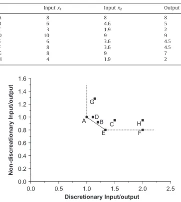
Inputs and output for the illustrative example .

Input x1 Input x2 Output y

A 8 8 8 B 6 4.6 5 C 3 1.9 2 D 10 9 9 E 6 3.6 4.5 F 8 3.6 4.5 G 8 9 7 H 4 1.9 2 1.6 1.4 1.2 1.0 0.8 0.6 0.4 0.2 0.0 0.0 0.5 1.0 1.5 2.0 2.5 Discretionary Input/output Non-discreationary Input/output A E F H C B D G

Fig. 1. Graphical representation for the illustrative example.

An alternative formulation for the CRS model of Banker and Morey [12] reproduced in (2) that has commonly been adopted in DEA studies only differs from the VRS formulation in (1) by removing the convexity constraint (Pn_j=1

k

_j=1). For example, Cooper et al.[14, p. 60]adopted this formulation in their textbook. The major difference between the original formulation of Banker and Morey[12]and the alternative formulation is that the latter assumes that the scale of the ND inputs can be adjusted. This implies that all inputs, outputs and ND factors need to be scale dependent, i.e., volume measures that can be scaled. In this paper we will only discuss the original formulation of the CRS model for dealing with ND factors, that assumes that ND factors cannot be scaled, irrespectively of being measured as volume variables or index type variables. For a detailed comparison of both formulations and the practical implications of their differences see Syrj¨anen[5].

The treatment of internal ND factors according to the approach of Banker and Morey[12]allows ND factors to define the PPS, and the VRS PPS is the same whether one considers the ND factors as such or whether one considers the ND factors as controllable. For the CRS case, however, the PPS changes when internal ND factors are treated as such rather than as discretionary factors. The fact that the PPS is maintained for the approach of Banker and Morey[12]under VRS has been criticized in the literature. For example Mu ˜niz[15]argues that, treated in this way, environmental conditions have no influ-ence on the units that define the efficient frontier, and only ineffi-cient DMUs can be penalized by the consideration of some factors as being ND. To see this, consider the illustrative example inTable 1 andFig. 1(from Vaz[16]), where we represent a situation where input 1 is discretionary and input 2 is ND (we assume that a higher value for this input is associated with more favorable environmental conditions). InFig. 1both inputs are normalized by the output.

Note that considering input 2 as a discretionary input would im-ply that DMUs A, E, and F were assigned a 100% CRS efficiency score, although DMU F is weakly efficient, as can be seen inFig. 1. If we con-sider input 2 ND, then the CRS results from the Banker and Morey

Table 2 Illustrative example . Eff./DMU A B C D E F G H CRS BM efficiency (%) 100.00 93.91 100.00 90 89.73 67.30 87.50 75.00 CRS DEA efficiency (%) 100.00 97.56 86.49 96.00 100.00 100.00 87.50 84.21 VRS BM efficiency (%) 100.00 98.02 100.00 100.00 100.00 75.00 89.58 75.00 VRS DEA efficiency (%) 100.00 98.92 100.00 100.00 100.00 100.00 89.58 100.00

[12] input oriented model are shown in Table 2 (labeled "BM efficiency''). This table also shows the efficiency scores that would be obtained if input 2 was considered discretionary (labeled "DEA efficiency''). Note that we present in this table both CRS and VRS results.

As can be seen in Table 2, the CRS frontier changed with the consideration of input 2 as ND, and some DMUs changed their status from inefficient to efficient (like C) and others lost their efficiency status (like E). For details on these changes see Thanassoulis et al. [4]. On the contrary, the VRS frontier is the same whether input 2 is considered discretionary or ND (note that DMUs F and H are assigned a 100% efficiency score in the VRS DEA efficiency inTable 2but they are weakly efficient).

Therefore the Banker and Morey[12]approach implies a change in the CRS frontier when internal ND factors are treated as such, but no change in the VRS efficient frontier in relation to the situation where all factors are considered discretionary. The reason for this is that under VRS the units are compared only with others of similar scale, and therefore the peer set is reasonable even for comparisons relating to the ND factor. Under CRS, however, the DMUs are allowed to be compared with every efficient unit in the data set, whatever its scale size, and this may be unfair for some DMUs since ND factors are not scalable. Therefore the frontier needs to be changed for the CRS case, but can be the same for the VRS assessment.

Golany and Roll [17] extended the CRS model of Banker and Morey[12]to consider simultaneously ND inputs and outputs. Ac-cording to Golany and Roll[17]a CRS model with both discretionary (D) and ND inputs (index i) and outputs (index r) is shown as

min   

h

hx

ij₀

>

When the final efficiency scores are intended to reflect not only differences in discretionary factors but also differences in external ND conditions, then single stage or multiple stage approaches can be used.

The approach proposed by Ruggiero[11]fits into the single stage approaches and consists on solving a DEA model restricting the ref-erence set for each DMU under evaluation to DMUs presenting only equal or more disadvantageous conditions in terms of the ND factor. The model has the following formulation (input oriented and VRS technology): min   

h

Although the ND factors are used in the formulation of the DEA model (4), these variables are not internal to the model. Since the convexity condition is not imposed on the ND inputs we can look at (4) as a model that assesses the efficiency of each production unit in relation to a traditional VRS frontier, where this frontier changes depending on the DMU being assessed (since for each DMU the peers are only those DMUs presenting worst or equal envi-ronmental conditions). In this sense, this approach is very similar to the approaches that group units according to some categorical factor and assess them in relation to different frontiers. In fact, the Ruggiero [11] model extends the model to treat ND categorical variables of Banker and Morey[10]to the case where ND factors are con-tinuous. To see this consider in Table 3 the results of Ruggiero

Table 3

Results of the Ruggiero[11]VRS model applied to the illustrative example .

DMU VRS efficiency (%) Peers Reference

A 100 kA=1 Frontier 4 B 100 kB=1 Frontier 3 C 100 kC=1 Frontier 1 D 100 kD=1 Frontier 5 E 100 kE=1 Frontier 2 F 75 kE=1 Frontier 2 G 89.6 kA=0.83,kC=0.17 Frontier 5 H 75 kC=1 Frontier 1 D A G B F E H C 0 2 4 6 8 10 0 10 12 Discretionary Input Output frontier 1 frontier 2 frontier 3 frontier 5 frontier 4 8 6 4 2

Fig. 2. Different VRS frontiers in Ruggiero's model for different DMUs[4].

[11] model applied to our illustrative example and Fig. 2 that shows the different VRS frontiers against which efficiency was measured.

The approach of Ruggiero[11], imposing more restrictive condi-tions on the peer set to ensure homogeneity among DMUs and to al-low fair comparisons, may overestimate efficiency and can lead to a high number of efficient units. This goes in line with the DEA spirit of showing units in the best possible light, but at the same time it may in fact restrict too much the reference set not allowing a clear dis-crimination between DMUs. See Syrj¨anen[5]for a simulation study comparing true efficiencies with efficiency estimates obtained with models accounting for ND factors.

Note, for example, that the approach of Ruggiero[11]may con-sider very small reference sets, such as that of DMUs C and H, or may consider very close efficient frontiers such as frontiers 2 and 3. One could argue that since the ND factor implicit in the con-struction of these two frontiers is very similar, a single frontier could be considered for assessing DMUs B, E and F. This rationale is behind the approach that we develop in this paper for treat-ing simultaneously internal and external ND factors. Note that as the number of ND factors increases, the probability of a unit be-ing rated efficient in model (4) also increases. In addition, with multiple ND variables the model of Ruggiero[11] ignores possible trade-offs between these variables (see Mu ˜niz et al.[21]). Recogniz-ing these problems, Ruggiero [18] proposed aggregating multiple ND factors through a regression analysis and modifying model (4) to consider the aggregated ND factor rather than individual ND factors.

More recently, Ruggiero [22] proposed an enhanced model to deal with ND factors that allows the DMU under evaluation to be compared with others that, within given limits, have more favor-able environmental conditions. These limits (

d

(x_i)) are established

for each ND input and correspond to the maximal values until which the comparisons are considered fair. The formulation of the model proposed by Ruggiero [22] is shown in (5). The value of

d

(xi) can be estimated using parametric techniques such as

(5)

regression: min   

j

>

0, j = 1, . . . , n    (5)

There is a panoply of other methods to deal with external ND factors, most of which consider multiple stage approaches. These approaches in general assess DEA efficiency using discretionary fac-tors only and then correct the efficiency scores obtained at further stages. Examples of such multi-stage approaches can be found in Fried et al.[23,24], Mu ˜niz[15], and Grosskopf et al.[25]. These meth-ods are beyond the scope of this paper, and will not be detailed here.

ND factors for explaining efficiency

In some cases ND factors can be used to explain differences in efficiency scores, and not to correct efficiency scores. This approach was introduced by Ray [26]and further developed in Ray [27] in an application to school districts. In Ray[26]the author run in a first stage a DEA model with discretionary factors only, and used in a second stage a regression model of the DEA efficiency scores on the ND variables. According to Ray[27], the shortfall of the DEA efficiency score from one (or 100% efficiency) includes the influence of ND factors and the influence of bad management (or managerial inefficiency). In order to estimate only the managerial inefficiency of a school district, the shortfall of the DEA efficiency score from the estimated regression score should be used. Such a difference is interpreted by Ray[27]as the extent of managerial inefficiency not caused by external factors.

The Ray[27]approach requires the specification of a functional form to the regression model meaning that a mis-specification may distort the results (see Ruggiero[18], McCarty and Yaisawarng[28]. One problem of using parametric techniques for explaining differ-ences in DEA efficiency relates to the possible correlation between the input and output factors used to calculate the DEA efficiency scores and the independent variables used in the regression model (see Grosskopf [29]). Another problem is that the DEA efficiency scores are dependent on each other, which "violates a basic assump-tion required by regression analysis: the assumpassump-tion of indepen-dence within the sample''[30, p. 3]. Note that two-stage models have been improved since Ray[27]to consider in the second stage Tobit models rather than traditional regression models to account for the fact that the dependent variable (the efficiency score) is bounded between 0 and 1. The use of Tobit models for explaining differences in DEA efficiency scores has been generalized, as testifies the ex-haustive list of studies using Tobit second stage models in Simar and Wilson[31]. However, the use of Tobit models cannot resolve the dependency problem mentioned above and, according to Simar and Wilson[31], they are invalid, in particular for inference. Bootstrap techniques can be used instead of Tobit models to explain differ-ences in efficiency. Examples of the application of bootstrap statis-tical techniques for explaining differences in efficiency can be found in Daraio and Simar[32]or Simar and Wilson[31].

Methodology for retail store assessment

This section describes a general DEA model developed to ac-commodate ND inputs and outputs. The treatment given to the ND

variables depends on their classification as internal or external to the production process. The generalized model developed in this pa-per integrates previous models, in particular the model by Banker and Morey[12] and its extension to both ND inputs and outputs by Golany and Roll[17], and the model of Ruggiero[11]and its ex-tension described in Ruggiero [22]. The model is called thereafter generalized model for non-discretionary factors or GMOND.

The GMOND model considers both external ND inputs and outputs in the selection of possible peers, and internal ND factors, together with discretionary ones, to define the PPS. Note that the as-signment of an external ND factor to the input or output category is based on its influence on the production process. The factor should be an input when it is fair to compare the DMU being assessed with DMUs having a lower level of this factor, and an output when the DMU being assessed should be compared with peers presenting higher values on that factor.

r< 1, ∀r,

k

j

>

0, ∀j (6)

The sets DI, IntNDI and ExtNDI are associated with discretionary, internal ND and external ND inputs, respectively. Similarly, DO, Int-NDO and ExtInt-NDO are the sets of discretionary, internal ND and external ND outputs.

d

0is a non-oriented measure of inefficiency.

(6)

Table 4

Some special cases for model (6) .

When Model (6) reduces to

gyr=0, gxi=xi0, IntNDO = ExtNDI = ExtNDO = ∅ Model of Banker and Morey[12]input oriented

gyr=yr0, gxi=0, IntNDI = ExtNDI = ExtNDO = ∅ Model of Banker and Morey[12]output oriented

gyr=0, gxi=xi0, ExtNDI = ExtNDO = ∅ Model of Golany and Roll[17]input oriented

IntNDI = IntNDO = ExtNDI = ExtNDO = ∅ Standard directional model

gyr=0, gxi=xi0, IntNDO = IntNDI = ExtNDO = ∅,ai=0 Model of Ruggiero[11]input oriented

gyr=0, gxi=xi0, IntNDO = IntNDI = ExtNDO = ∅,aiparametrically defined Model of Ruggiero[22]input oriented

g = (g_xi, gyr) is a directional vector chosen a priori. Restrictions (6a)--(6e) define the PPS and restrictions (6f) and (6g) define the peer set against which the unit j0is being assessed. Restrictions (6a) and (6b) are the standard restrictions in a DEA directional model, restrictions (6c) and (6d) are the standard restrictions to model in-ternal ND factors according to the procedure of Banker and Morey [12], restriction (6e) is the standard restriction imposing that the technology is VRS, and (6f) and (6g) are an adapted version of the re-strictions associated with peer selection in Ruggiero[11,22]models. For

a

_i=0, restriction (6f) is identical to the restriction of Ruggiero [11]model reproduced in (4). Values of

a

i> 0 or

b

r> 0 enable peers to have more favorable external conditions than the DMU assessed, provided that the more favorable conditions are within sensible lim-its defined by the decision maker. The definition of the margins in percentage terms and in line with decision maker's opinion is con-ceptually simpler than their parametrically calculated equivalents in Ruggiero[22], making them intuitively more appealing.

In F¨are and Grosskopf[35]the authors specified the directional vector as being equal to the observed inputs and outputs, which made it possible to show the equivalence between the traditional DEA input and output efficiency models and the directional model. For a directional vector implying an input oriented assessment g =

(x_i₀, 0), the radial DEA efficiency measure is equivalent to (1 −

d

0). Similarly, for an output oriented directional vector g = (0, yr₀), the radial DEA efficiency measure is equivalent to 1/(1 +

d

0). Note that the directional distance models are units invariant when the direc-tional vector corresponds to the observed inputs and outputs of the DMU under assessment. However, if the directional vector is iden-tical for all DMUs, then the model is not units invariant.Table 4 notes the equivalences between model (6) and other models in the literature.

Constraints (6f) and (6g) are not standard constraints of linear programming. However, a simple computational framework for solv-ing model (6) would be to pre-identify all potential comparators for a given DMU, and then only consider those peers for solving a linear programming model without constraints (6f) and (6g). In our case we used GAMS and were able to implement the above model easily and through a single step procedure. Details on the GAMS models used can be provided to the interested reader upon request. For de-tails on the use of GAMS for DEA see Olesen and Petersen[36].

Note that in the presence of several ND factors, the GMOND model suffers from the same problems as the models of Ruggiero [11,22]where insufficient discrimination between DMUs may arise due to very limited comparative sets. Golany and Roll[17]also men-tion the possible problems that may occur when a dispropormen-tionate number of ND factors are included into the analysis. In such cases, we recommend the use of only those discretionary factors that are believed to have a true impact on performance (which can be in-vestigated through statistical techniques after DEA efficiencies have been computed). In alternative, ND factors can be aggregated in a way that represents the context that DMUs face on various external conditions. In this paper, for example, we replace two external ND factors (population and competition) by only one ND factor that is a ratio between the two contextual variables. We do this aggregation

i< 1, ∀i, 0

6b

r< 1, ∀r,

k

j

>

0, ∀j

A generalized model that combines several formulations to deal with ND factors has previously been reported in Syrjänen[5]. How-ever, the emphasis of the model in Syrjänen[5]is to provide differ-ent formulations for the restrictions concerning inputs and outputs measured in different scales. Some restrictions are suitable for fac-tors of volume type, whereas others are suitable for index indicafac-tors. According to Syrjänen [5], for VRS models, there is no distinction between the treatment given to volume type factors or index type factors, as the variables cannot be scaled up or down. However, for CRS only the volume type variables can be scaled. In addition, the model distinguishes discretionary inputs and outputs from ND fac-tors, such that only discretionary factors are included in the projec-tion to derive the efficiency measure.

There are several similarities between the GMOND model pro-posed in this paper and the model in Syrj¨anen [5]. Both use the ideas underlying directional distance functions, such that by defin-ing the parameters of a directional vector different projections to the frontier are achieved. However, the restrictions specified in GMOND distinguish the variables that are under managerial control from non-controllable factors. All controllable factors are assumed to be volume-type inputs and outputs, such that either a CRS or VRS as-sumption can be imposed to these variables. The non-controllable factors are either allowed to define the shape of the PPS, in case they are internal to the production process, but we assume their value is fixed, such that no scale adjustments are possible (and thus are treated as the index variables in Syrj¨anen[5]). Finally, the external

(7)

ND factors are not allowed to define the shape of the PPS, so the re-strictions associated to these variables are a generalized version of the Lovell--Ruggiero restrictions described in Syrj¨anen[5, p. 31].

Empirical application

The Portuguese retail sector

The Portuguese retail sector is nowadays a mature sector, whose importance to the Portuguese economy increased significantly in the past few years, rising from a volume of business of 2634 million eu-ros in 1988 to 10 710 million eueu-ros in 2005 (according to the retailing statistics compiled by the company AC Nielsen). The sector is dom-inated by five commercial groups, two Portuguese (Sonae, Jer ´onimo Martins) and three French (Intermache, Auchan, Carrefour). Compe-tition is high, and has been intensified by the entrance in the market of discount stores. The balance between the number of traditional grocery stores and the number of stores with modern formats (i.e., supermarkets and hypermarkets with large sales areas) parallels the levels observed in Europe (according to the Portuguese Association of Retailing Companies---APED, the average market share of stores with modern formats in Portugal is 78% and in Europe is 86%).

In this highly competitive context, the pressure on sales margins reduction demands for additional efforts to rationalize processes and increase operations control, as well as to improve customer services and to maintain a loyal relation with costumers. This makes efficiency assessment and improvement a key objective of retail organizations.

Performance assessment of retailing organizations using DEA

The DEA literature includes several studies concerning the per-formance assessment of retail outlets. However, the number of stud-ies focusing specifically on supermarket stores is limited. Some of these studies focused on the performance of individual stores from the same chain[37--39], and others compared the performance of supermarket chains[40].

Athanassopoulos and Ballantine[40]used DEA to compare the ef-ficiency of supermarket chains operating in the United Kingdom. The inputs included capital employed, fixed assets, number of employ-ees, number of outlets and sales area. The output included total sales. Barros and Alves[37]used Malmquist indices to estimate produc-tivity change and decomposed it into technical efficiency change and technological change. The analysis explored 47 supermarkets oper-ating in Portugal in the years 1999 and 2000. The inputs included number of full-time equivalent employees, cost of labor, number of cash-out points, stock and other costs. The outputs included sales and operational results.

Ket and Chu[38]assessed the performance of 13 supermarkets for 10 years, using a three-stage approach. The first stage analyzed the transformation of raw materials (labor and capital) into a set of intermediate outputs (five distribution services). The second stage explored the connection between the distribution services and the final output (sales revenue). Finally, stage 3 examined the relation-ship between the raw inputs and the final output.

Korhonen and Syrj¨anen[39]assessed the performance of a super-market chain in Finland with 25 stores. The inputs considered were the number of staff working hours and the area of the supermarket. The outputs were total sales and profit. The main objective of the assessment was to realocate the resources available for the chain among the supermarkets, allowing for an increase in resources that could not exceed a given limit. The first model explored resource reallocations keeping the current mix of inputs and outputs, as well as the efficiency levels observed. The second model explored real-locations with different assumptions: the area of the store and the

efficiency levels should remain with their current values, and only staff working hours could be allocated among the stores to maximize sales and profit.

It should be noticed that previous studies on supermarket efficiency did not incorporate external ND variables in the DEA assessments. However, this has been pointed as a limitation of these studies that, in most cases, could not be overtaken due to the difficulties in collecting appropriate data to capture the essence of contextual conditions[41].

Conversely, the studies that assessed retail outlets from organiza-tions operating in non-food related sectors tended to incorporate ND variables in the analysis, such as location and age of the store, pop-ulation density, average family income or competition in the catch-ment area. For example, Donthu and Yoo[42]and Thomas et al.[43] included the ND factors in the DEA using the Banker and Morey[12] model, whereas Grewal et al. [44] used the model in Banker and Morey[10]. Norman and Stoker[45]used standard DEA models with an output orientation and incorporated the ND factors as inputs.

In relation to the DEA assessments of retailing outlets, an im-portant feature of the analysis reported in the literature relates to the involvement of managers in the selection of the inputs and out-puts, as well as in the interpretation of the results. For example, in the study by Thomas et al.[43]the decision maker opinion on the importance of the inputs and outputs was incorporated in the DEA model using weight restrictions. The importance of an appropriate selection of inputs and outputs for retailing assessments, as well as the interest of distinguishing between discretionary and ND factors, was also noted in Donthu and Yoo[42].

The assessment reported in this paper followed some of the main features identified in the retailing literature review. More specifi-cally, the inputs and outputs used in the assessment were defined with the collaboration of the managers responsible for performance planning and control of the supermarket chain under analysis. Also, their opinion in relation to the impact of external ND variables on store activity was important to define suitable margins for peer se-lection in order to ensure a fair comparison between stores.

Description of the retailing organization

We applied the aforementioned model to assess the efficiency of supermarkets and hypermarkets from a chain operating in Portugal. The layout of the stores is organized into five sections: grocery, per-ishables, light bazaar, heavy bazaar and textiles. The objective of this paper is to evaluate the efficiency of stores in generating sales, taking into account the resources available (both discretionary and ND) and the external ND factors that characterize the store catchment area. The results reported in this paper were computed using 70 stores in total, 14 hypermarkets and 56 supermarkets. The supermarkets con-sidered are large and their activity is comparable to the hypermar-kets, which ensures the homogeneity of the sample considered. The organization also owns a chain of small size supermarkets, located in residential areas, but these were excluded from the assessment.

As illustrated inFig. 3, the inputs of the DEA model are the floor area (m2), the value of the products in stock (Ł), the operational costs (Ł), the staff costs (Ł), the value of the products spoiled (Ł) and the ratio of population/competition to reflect the external environmental conditions of the stores. The output of the model is the value of sales (Ł).

The floor area of the store represents its size, which has a di-rect influence on the volume of sales. We assume that the area of a store is not controllable in the short run and therefore consider this input as ND. This ND factor is, however, internal to the produc-tion process. The stock is the value of the products that each store has available to sell. The operational costs include the costs associ-ated with logistics, advertising campaigns, maintenance, electricity,

(8)

Discretionary factors Internal ND factors External ND factors Stock Operational costs Staff costs Products spoiled Area Population Competition

Store Value of sales

Fig. 3. Inputs and outputs of the GMOND DEA model.

communications, security and cleaning services. The staff costs are the wages paid to the employers that work in the store. The prod-ucts spoiled relates to the amount lost with prodprod-ucts stolen, spoiled or whose validity expired. Although this variable is a result of the activity of the store, it is an undesirable output that the store wants to minimize. There are several alternatives for including this type of data in the DEA models (see Dyson et al.[46]). The variable can be included in the model as an input, it can be deducted from a large constant, or it can be inverted. The last two alternatives mod-ify the measurement scale, which can make the interpretation of the results difficult. Thus, including the undesirable output as an input of the model was considered the best option for the analysis re-ported in this paper, such that stores with higher values of products spoiled are penalized in the DEA assessment. The output is the value of sales, which reflects both the amount of products sold and their prices. Note that by including a composed measure of quantities an prices on the output side we are implicitly assuming that prices are endogenous, so that movements towards the efficient frontier can be accomplished either through changes in quantities or through changes in prices. In the case of the stores analyzed, the prices of most products are set centrally by the organization. As a result, most stores practice very similar prices, meaning that differences in ef-ficiency pertain mainly to differences in quantities of outputs sold rather than to differences in their prices.

The company used as case study considers that the population and the competition are the most critical external ND factors that influence store activity. The population density has a positive im-pact on sales. This variable is measured by the inhabitants living in municipalities within half-hour distance from the store (this time is calculated considering an average speed of 50 km/h). In opposition, the competition has a negative contribution to the volume of sales. This variable is measured by the floor space of competitive stores within half-hour distance from the store. The company uses the ratio population over competition when it is important to contextualize the store environmental conditions in performance evaluations. We also used the ratio population over competition as the external ND factor, in order to take into account the effect of both variables in the DEA.

Table 5shows the summary statistics of the inputs and outputs of the 70 stores analyzed.

The standard deviation of all variables is quite high relative to the mean, indicating a considerable amount of diversity in the stores of the organization analyzed. This motivated the use of a VRS model for the efficiency assessment, to increase the comparability between the inefficient stores and the peers in terms of scale size. Another reason for using VRS relates to restrictions imposed by Portuguese legislation, that forces stores with more than 2000 m2to be closed on Sunday afternoons and bank holidays. As a result, the supermarkets are often kept below this size threshold to enable them to open without restrictions. It is therefore to be expected that stores face some scale inefficiencies. This was in fact confirmed in a wider study of these stores, in Vaz[16], from which this paper reports only a part.

Table 5

Mean and standard deviation for the inputs and outputs of the stores .

Mean Standard deviation

Discretionary inputs

Stock (euros) 2 640 902 2 205 246

Operational costs (euros) 1 307 480 1 439 545

Staff costs (euros) 1 965 931 1 935 089

Products spoiled (euros) 476 187 486 497

Internal non-discretionary input

Area (m2₎ ₄₁₇₁ ₃₁₉₉

External non-discretionary input

Populationa_/competitionb _13.8 _9.9

Discretionary output

Sales (euros) 34 345 028 35 829 888

a_{The population mean is 54 109 and the standard deviation is 61 497.} b_{The competition mean is 4428 and the standard deviation is 4804.}

These scale inefficiencies can be considered a case of rational scale inefficiency in the sense of Bogetoft and Hougaard[47]. That is, stores rationally choose not to look for scale efficiency since achieving scale efficiency has a cost, and when this is accounted for, inefficiency may be less costly than the effort to achieve scale efficiency.

Results

This section describes the results obtained in the store efficiency assessment taking into account the effect of ND factors. We first present the results of the GMOND model distinguishing between discretionary and ND factors, both internal and external, as classified inTable 5. The sensitivity of the model to the values of

a

i is also tested.

The results of the GMOND model are compared with those of a DEA model without including the effect of external ND factors. This analysis aims to evaluate the impact of the external conditions on store activity: those stores whose efficiency estimate is higher in the GMOND model with peer selection restrictions (6f) and (6g) than with the model only with restrictions (6a)--(6e) are the ones most critically affected by the contextual conditions in the surrounding area.

Finally, the differences in the efficiency estimates associated with the treatment of floor space as an internal ND factor versus the treatment as a discretionary factor are also explored.

Store efficiency results

Table 6reports the results of the GMOND model obtained with a directional vector g = (x_ij

0, yrj0) and using the input and output factors as classified inTable 5. The criteria used for peer selection was having the external ND input (i.e., the ratio population/competition)

(9)

Table 6

Results ofd0in model (6) for distinct values ofa.

a=25% a=20% a=15% a=10% a=5% a=0% Average inefficiency (d0) (%) 2.2 2.2 2.1 2.0 2.0 1.8 Standard deviation (%) 3.0 3.0 2.9 2.8 2.8 2.7 No. of efficient DMUs (withd0=0) 34 36 36 37 38 39 Maximum inefficiency score (%) 11.1 11.1 11.1 11.1 11.1 10.4 Table 7

Comparison of results witha=20% and 0% for store L50 .

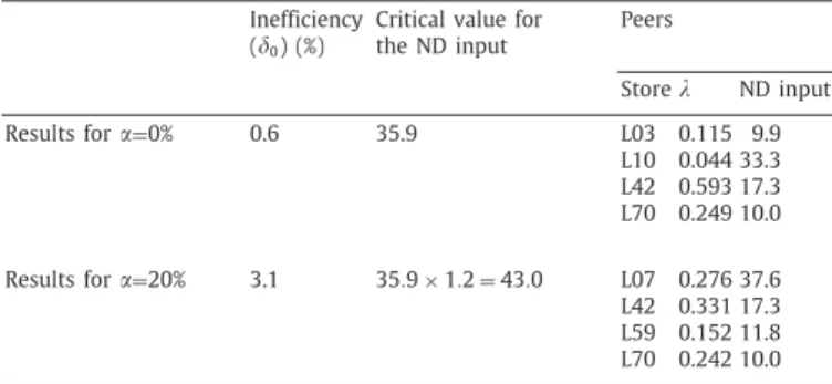
Inefficiency (d0) (%)

Critical value for the ND input

Peers

Storek ND input

Results fora=0% 0.6 35.9 L03 0.115 9.9

L10 0.044 33.3 L42 0.593 17.3 L70 0.249 10.0 Results fora=20% 3.1 35.9 × 1.2 = 43.0 L07 0.276 37.6 L42 0.331 17.3 L59 0.152 11.8 L70 0.242 10.0

equal or lower than 1.2 times the value of this ratio in the store assessed, which corresponds to

a

=20%. This value was arrived at in consultation with company managers and it was agreed that this would be a reasonable threshold.Table 6 presents the results of model (6) with

a

=20% and 0% we discuss one illustrative example, corresponding to store L50 (with a value of the external ND input equal to 35.9).Table 7 reports the efficiency measures, the value of the ND input for the peers, and the critical value for the ND input beyond which other DMUs are not allowed to be part of the peer set.

The model with

a

=0% evaluates store L50 as almost efficient, whilst for

a

=20% the assessment estimates an inefficiency of 3.1%.

0% 5% 10% 15% 20% 25% DMUs In e ff ic ie n c y

Ignoring External ND factors With External ND factors (alfa =20%)

Fig. 4. Inefficiency distributions with external ND factors and ignoring external ND factors.

This is because the discrimination of the DEA model improves con-siderably due to the enlargement of the set of potential peers asso-ciated with the use of a value of

Fig. 4illustrates the inefficiency distributions (

d

0) associated with the use of model (6) with

a

=20%, and the results without accounting for external variables.

We can conclude that the results of the two DEA models are quite different. Fifty one (out of 70) stores increased their efficiency estimate with the evaluation using model (6) accounting for external ND factors. In particular, 18 of these stores changed their status from inefficient to efficient, meaning that when the effect of the environmental conditions is taken into account, there is no evidence that their performance can be further improved.

For the 19 stores whose score was identical in the two models, 18 stores are efficient in both models, and only 1 is equally ineffi-cient in the two models. This indicates that the peers used in the DEA model without accounting for the external ND conditions al-ready had environmental conditions comparable to the DMUs under evaluation.

The gap between the inefficiency estimates of the two formula-tions was under 5% for the majority of stores.

(10)

There are two cases worth noting, relating to stores L44 and L14. These stores had, respectively, inefficiency estimates

d

0=9.3% and 20% ignoring the effect of external ND factors, and were considered efficient when the model accounted for their influence. Store L14 faces one of the worst environmental conditions, such that only two DMUs are allowed as potential peers using model (6). This in-dicates that the high efficiency score of this DMU may be due to the small peer set available in the sample analyzed. However, the case of store L44 is quite different. The environmental conditions faced by this store are quite good, such that the set of potential peers in model (6) includes 63 stores for a value of

a

=20%. Therefore, the classification of this store as efficient cannot be attributed to the non-existence of appropriate comparators, but should be inter-preted as an evidence that it is not possible to obtain higher sales given the level of resources available and the external conditions of the store catchment area.

Comparing the results of model (6) treating area as an internal ND input versus a model treating area as a discretionary input, in both cases with

a

=20% in the restriction concerning the external factors, we found that the differences in the inefficiency estimates are very small. The inefficiency estimate decreased for 15 DMUs when the area was considered as a discretionary input. However, the differences between the inefficiency scores were below 1% for 13 DMUs, and just slightly above 1% for the other two DMUs (1.1% for L26 and 1.9% for L21). Therefore, the impact of considering area as an internal ND input is marginal, in particular when we compare this impact with that of taking into account the external ND factor in the estimation of efficiency.

Conclusions

This paper proposes a new model to assess the performance of DMUs in the presence of ND factors. The new model constructs the PPS based only on discretionary factors and internal ND factors, and implements a procedure for peer selection according to the values of the external ND factors. This new model integrates the existing approaches for dealing with ND variables described in the DEA lit-erature, based on a typology that suggests different treatments de-pending on the classification of the ND factors as internal or external to the production process.

The procedure described in this paper estimates inefficiency based on a directional distance function and is not restrictive in comparing DMUs to peers with strictly less favorable levels of the external ND factors. It allows for a comparison of the DMU being assessed with peers presenting more favorable levels of the ND factor within certain limits. These limits, that are in fact the peer selection criteria, can be defined by the decision maker/analyst.

In terms of the results of the retail stores' assessment, the analysis identified 36 inefficient stores when the effect of both internal and external ND conditions is taken into account. For these stores, the average level of inefficiency was 2.2%. We found that the inefficiency estimates were quite sensible to the exclusion of the external ND factors from the assessment, so the use of the model developed in this paper was essential for obtaining unbiased efficiency estimates. However, for the stores analyzed, the impact of considering the floor space as an internal ND variable or as a discretionary factor was not very significant.

The performance of the retail stores can also be influenced by the format of the store (hypermarkets or supermarkets). Although exploring this issue was beyond the scope of this article, the impor-tance of this topic recommends its analysis in future research.

References

[1]Desmet P, Renaudin V. Estimation of product category sales responsiveness to allocated shelf space. International Journal of Research in Marketing 1998;15(5):443--57.

[2]Campo K, Gijsbrechts E. Should retailers adjust their micro-marketing strategies to type of outlet? An application to location-based store space allocation in limited and full-service grocery stores. Journal of Retailing and Consumer Services 2004;11:369--83.

[3]Charnes A, Cooper WW, Rhodes E. Measuring the efficiency of decision making units. European Journal of Operational Research 1978;2(6):429--44. [4]Thanassoulis E, Portela M, Despic O. DEA---the mathematical programing

approach to efficiency analysis. In: Fried HO, Lovell CAK, Schmidt SS, editors. Second edition of the measurement of productive efficiency: techniques and applications. New York, Oxford: Oxford University Press; 2007.

[5]Syrj¨anen MJ. Non-discretionary and discretionary factors and scale in data envelopment analysis. European Journal of Operational Research 2004;158: 20--33.

[6]Charnes A, Cooper WW, Rhodes E. Evaluating program and managerial efficiency: an application of data envelopment analysis to program follow through. Management Science 1981;27(6):668--97.

[7]Berger SA, FZrsund FR, Hjalmarsson L, Suominen M. Banking efficiency in the Nordic countries. Journal of Banking and Finance 1993;17:371--88.

[8]Pastor JM, P´erez F, Quesada J. Efficiency analysis in banking firms: an international comparison. European Journal of Operational Research 1997;98:395--407.

[9]Camanho AS, Dyson RG. Data envelopment analysis and Malmquist indices for measuring group performance. Journal of Productivity Analysis 2006;26(1): 35--49.

[10]Banker RD, Morey RC. The use of categorical variables in data envelopment analysis. Management Science 1986;32(12).

[11]Ruggiero J. On the measurement of technical efficiency in the public sector. European Journal of Operational Research 1996;90:553--65.

[12]Banker RD, Morey RC. Efficiency analysis for exogenously fixed inputs and outputs. Operations Research 1986;34(4):513--21.

[13]Banker RD, Charnes A, Cooper WW. Some models for estimating technical and scale inefficiencies in data envelopment analysis. Management Science 1984;30(9):1078--92.

[14]Cooper WW, Seiford LM, Tone K. Introduction to data envelopment analysis and its uses: with DEA-solver software and references. USA: Springer Science; 2006.

[15]Mu ˜niz MA. Separating managerial inefficiency and external conditions in data envelopment analysis. European Journal of Operational Research 2002;143: 625--43.

[16]Vaz CB. Development of a performance assessment and improvement system in the retailing sector. PhD thesis, University of Porto, Portugal, 2007. [17]Golany B, Roll Y. Some extensions of techniques to handle non-discretionary

factors in data envelopment analysis. Journal of Productivity Analysis 1993;4: 419--32.

[18]Ruggiero J. Non-discretionary inputs in data envelopment analysis. European Journal of Operational Research 1998;111:461--9.

[19]Staat M. Treating non-discretionary variables one way or the other: implications for efficiency scores and their interpretation. In: Westermann G, editor. Data envelopment analysis in the service sector. Gabler Edition Wissenschaft; 1999. p. 23--49.

[20]Yang Z, Paradi JC. Cross firm bank branch benchmarking using "handicapped'' data envelopment analysis to adjust for corporate strategic effects. In: Proceedings of the 39th Hawaii international conference on systems sciences, Hawaii, 2006.

[21]Mu ˜niz M, Paradi J, Ruggiero J, Yang Z. Evaluating alternative DEA models used to control for non-discretionary inputs. Computers & Operations Research 2006;33(5):1173--83.

[22]Ruggiero J. Performance evaluation when non-discretionary factors correlate with technical efficiency. European Journal of Operational Research 2004;159(1):250--7.

[23]Fried HO, Schmidt SS, Yaisawarng S. Incorporating the operating environment into a nonparametric measure of technical efficiency. Journal of Productivity Analysis 1999;12:249--67.

[24]Fried HO, Lovell CAK, Schmidt SS, Yaisawarng S. Accounting for environmental effects and statistical noise in data envelopment analysis. Journal of Productivity Analysis 2002;17:157--74.

[25]Grosskopf S, Hayes K, Taylor L, Weber W. Budget-constrained frontier measures of fiscal equality and efficiency in schooling. The Review of Economics and Statistics 1997;79:116--24.

[26]Ray SC. Data envelopment analysis, nondiscretionary inputs and efficiency: an alternative interpretation. Socio-Economic Planning Sciences 1988;22(4): 167--76.

[27]Ray SC. Resource-use efficiency in public-schools---a study of Connecticut data. Management Science 1991;37(12):1620--8.

[28]McCarty TA, Yaisawarng S. Technical efficiency in New Jersey school districts. In: Fried HO, Lovell CAK, Schmidt SS, editors. The measurement of productive efficiency: techniques and applications. New York, Oxford: Oxford University Press; 1993. p. 271--87.

[29]Grosskopf S. Statistical inference and nonparametric efficiency: a selective survey. Journal of Productivity Analysis 1996;7:161--76.

[30]Xue M, Harker PT. Extensions of modified DEA. Working Paper 99-07, Wharton Financial Institutions Center, 1999.

[31]Simar L, Wilson PW. Estimation and inference in two-stage, semi-parametric models of production processes. Journal of Econometrics 2007;136(1):31--64. [32]Daraio C, Simar L. Introducing environmental variables in nonparametric

frontier models: a probabilistic approach. Journal of Productivity Analysis 2005;24:93--121.

(11)

[33]Chambers RG, Chung Y, F¨are R. Profit, directional distance functions, and Nerlovian efficiency. Journal of Optimization Theory and Applications 1998;98:351--64.

[34]Chambers R, Chung Y, F¨are R. Benefit and distance functions. Journal of Economic Theory 1996;70:407--19.

[35]F¨are R, Grosskopf S. Theory and application of directional distance functions. Journal of Productivity Analysis 2000;13:93--103.

[36]Olesen OB, Petersen NC. A presentation of GAMS for DEA. Computers & Operations Research 1996;23(4):323--39.

[37]Barros CP, Alves C. An empirical ana1lysis of productivity growth in a Portuguese retail chain using Malmquist productivity index. Journal of Retailing and Consumer Services 2004;11:269--78.

[38]Ket HT, Chu S. Retail productivity and scale economies at the firm level: a DEA approach. Omega 2003;31:75--82.

[39]Korhonen P, Syrj¨anen MJ. Resource allocation based on efficiency analysis. Management Science 2004;50(8):1134--44.

[40]Athanassopoulos AD, Ballantine JA. Ratio and frontier analysis for assessing corporate performance: evidence from the grocery industry in the UK. Journal of the Operational Research Society 1995;46:427--40.

[41]Kumar V, Karande K. The effect of retail store environment on retailer performance. Journal of Business Research 2000;49:167--81.

[42]Donthu N, Yoo B. Retail productivity assessment using data envelopment analysis. Journal of Retailing 1998;74(1):89--105.

[43]Thomas RR, Barr RS, Cron WL, Slocum JW. A process for evaluating retail store efficiency: a restricted DEA approach. International Journal of Research in Marketing 1998;15(5):487--503.

[44]Grewal D, Levy M, Mehrotra A, Sharma A. Planning merchandising decisions to account for regional and product assortment differences. Journal of Retailing 1999;75(3):405--24.

[45]Norman M, Stoker B. Data envelopment analysis: the assessment of performance. Chichester: Wiley; 1991.

[46]Dyson RG, Allen R, Camanho AS, Podinovski VV, Sarrico CS, Shale EA. Pitfalls and protocols in DEA. European Journal of Operational Research 2001;132:245--59. [47]Bogetoft P, Hougaard JL. Rational inefficiencies. Paper presented at the exclusive