Measurement of the differential and double-differential Drell-Yan cross sections in proton-proton collisions at $\sqrt{s} =$ 7 TeV

EUROPEAN ORGANIZATION FOR NUCLEAR RESEARCH (CERN)

CERN-PH-EP/2013-168 2013/12/17

CMS-SMP-13-003

Measurement of the differential and double-differential

Drell–Yan cross sections in proton-proton collisions at

_√

s

=

7 TeV

The CMS Collaboration

Abstract

Measurements of the differential and double-differential Drell–Yan cross sections are presented using an integrated luminosity of 4.5 (4.8) fb−1 in the dimuon (dielectron) channel of proton-proton collision data recorded with the CMS detector at the LHC at

√

s = 7 TeV. The measured inclusive cross section in the Z-peak region (60–120 GeV)

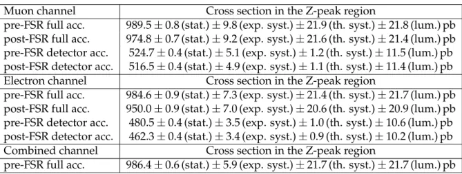
is σ(``) = 986.4±0.6 (stat.)±5.9 (exp. syst.)±21.7 (th. syst.)±21.7 (lum.) pb for the combination of the dimuon and dielectron channels. Differential cross sections dσ/dm for the dimuon, dielectron, and combined channels are measured in the mass range 15 to 1500 GeV and corrected to the full phase space. Results are also pre-sented for the measurement of the double-differential cross section d2σ/dm d|y| in the dimuon channel over the mass range 20 to 1500 GeV and absolute dimuon rapid-ity from 0 to 2.4. These measurements are compared to the predictions of perturbative QCD calculations at next-to-leading and next-to-next-to-leading orders using various sets of parton distribution functions.

Published in the Journal of High Energy Physics as doi:10.1007/JHEP12(2013)030.

c

2013 CERN for the benefit of the CMS Collaboration. CC-BY-3.0 license

∗_{See Appendix A for the list of collaboration members}

Contents 1

Contents

1 Introduction . . . 2

2 CMS detector . . . 3

3 Data and Monte Carlo samples . . . 3

4 Cross section measurements . . . 4

4.1 Event selection . . . 5

4.2 Background estimation . . . 7

4.3 Resolution and scale corrections . . . 10

4.4 Efficiency . . . 12

4.5 Acceptance . . . 14

4.6 Final-state QED radiation effects . . . 15

4.7 Systematic uncertainties . . . 16

5 Results and discussion . . . 25

5.1 Differential cross section dσ/dm measurement . . . . 25

5.2 Double-differential cross section d2σ/dm d|y|measurement . . . 30

6 Summary . . . 35

1

Introduction

The Drell–Yan (DY) lepton pair production in hadron-hadron collisions is described in the stan-dard model by s-channel γ∗/Z exchange. Theoretical calculations of the differential cross sec-tion dσ/dm and the double-differential cross secsec-tion d2σ/dm d|y|, where m is the dilepton invariant mass and|y|is the absolute value of the dilepton rapidity, are well established up to next-to-next-to-leading order (NNLO) in quantum chromodynamics (QCD) [1–4]. The rapid-ity distributions of the gauge bosons γ∗/Z are sensitive to the parton content of the proton, and the very high energy of the Large Hadron Collider (LHC) allows the parton distribution functions (PDFs) to be probed in a wide region of Bjorken x and Q2_{: 0.0003 < x < 0.5 and}

500< Q2 _{< 90000 GeV}2_{in the double-differential cross section measurement. The differential}

cross section dσ/dm is measured in an even higher Q2region up to 1.2×106GeV2. The large center of mass energy at the LHC allows a substantial extension of the range of Bjorken x and

Q2covered compared to previous experiments [5–10].

The rapidity y and the invariant mass m of the dilepton system produced in proton-proton col-lisions are related at leading order (LO) to the momentum fraction x+(x−) carried by the parton

in the forward-going (backward-going) proton as described by the formula x± = (m/

√

s)e±y_,

where the forward direction is defined as the positive z direction of the CMS detector coordi-nate system. Therefore, the rapidity and mass distributions are sensitive to the PDFs of the interacting partons. Since the y distribution is symmetric around zero in proton-proton col-lisions, we consider only the differential cross section in |y| in order to reduce the statistical errors. The measurements of the double-differential cross section d2σ/dm d|y|in DY produc-tion are particularly important since they provide quantitative tests of perturbative QCD and help to constrain the quark and antiquark flavor content of the proton. Precise experimen-tal measurements of these cross sections also allow comparisons to different PDF sets and the underlying theoretical models and calculations [11]. In addition, measuring DY lepton-pair production is important for other LHC physics analyses because it is a major source of back-ground for various interesting processes, such as tt and diboson production, as well as for searches for new physics beyond the standard model, such as the production of high-mass dilepton resonances.

The existing PDFs are derived from fixed-target and collider measurements of deep inelastic scattering (DIS), neutrino-nucleon scattering, inclusive jet production, and vector boson pro-duction from H1 and ZEUS [5], SLAC [6], FNAL E665, E772, E866 [7, 8], and the CDF and D0 [9, 10] experiments. These experiments covered the following ranges of dilepton invariant

mass and Bjorken scale parameter x: m ≤ 20 GeV and x > 0.01. Previous DY measurements

from the fixed-target experiments contributed substantially to the understanding of the quark and antiquark distributions in the proton. Collider vector boson production data contribute to constraining the d/u ratio at high x and the valence quark distributions. These data are also important in reducing the theoretical uncertainties in the determination of the W-boson mass at hadron colliders [12]. The current status of the PDFs and the importance of the LHC measure-ments are reviewed in Ref. [13, 14], and the DY differential cross section has been measured by CMS, LHCb, and ATLAS [15–17].

This paper presents measurements of the DY differential cross section dσ/dm in the dimuon and dielectron channels in the mass range 15<m<1500 GeV and the double-differential cross section d2σ/dm d|y|in the dimuon channel for the mass range 20 < m < 1500 GeV. These measurements are performed with the Compact Muon Solenoid (CMS) detector at the LHC using proton-proton collision data at√s= 7 TeV. The differential cross section measurements are normalized to the Z-peak region (60–120 GeV). This normalization cancels out the effect

3

of multiple interactions per bunch crossing (pileup) on the reconstruction, and the uncertainty in the integrated luminosity, acceptance, and efficiency evaluation. The measurements in this paper are corrected for the effects of resolution, which cause event migration between bins in mass and rapidity. The observed dilepton invariant mass is also corrected for final-state photon radiation (FSR). This effect is most pronounced below the Z peak. The differential cross sections are measured separately for both lepton flavors within the detector acceptance and are extrapolated to the full phase space. The consistency of the muon and electron channels enables them to be combined and compared with the NNLO QCD predictions calculated with

FEWZ [18] using the CT10 PDF set. The d2σ/dm d|y|measurement is compared to theFEWZ

next-to-leading-order (NLO) prediction calculated with CT10 PDFs and the NNLO theoretical

predictions as computed with FEWZ using the CT10, NNPDF2.1, MSTW2008, HERAPDF15,

JR09, ABKM09, and CT10W PDFs [19–25].

2

CMS detector

A right-handed coordinate system is used in CMS, with the origin at the nominal collision point, the x axis pointing to the center of the LHC ring, the y axis pointing up (perpendicular to the LHC plane), and the z axis along the counterclockwise-beam direction. The azimuthal angle φ is the angle relative to the positive x axis measured in the x-y plane. The central fea-ture of the CMS detector is a superconducting solenoid providing an axial magnetic field of 3.8 T and enclosing an all-silicon inner tracker, a crystal electromagnetic calorimeter (ECAL), and a brass/scintillator hadron calorimeter. The tracker is composed of a pixel detector and a silicon strip tracker, which are used to measure charged-particle trajectories covering the full azimuthal angle and pseudorapidity interval |η| < 2.5. The pseudorapidity η is defined as η = −ln[tan(θ/2)], where cos θ = pz/p. Muons are detected in the pseudorapidity range |η| < 2.4 with four stations of muon chambers. These muon stations are installed outside the solenoid and sandwiched between steel layers, which serve both as hadron absorbers and as a return yoke for the magnetic field flux. They are made using three technologies: drift tubes (DT), cathode strip chambers (CSC), and resistive-plate chambers. The muons associated

with the tracks measured in the silicon tracker have a transverse momentum (pT) resolution

of about 1–6% in the muon pT range relevant for the analysis presented in this paper.

Elec-trons are detected using the energy deposition in the ECAL, which consists of nearly 76 000 lead tungstate crystals that are distributed in the barrel region (|η| < 1.479) and two endcap regions (1.479 < |η| < 3). The ECAL has an ultimate energy resolution better than 0.5% for

unconverted photons with transverse energies (ET) above 100 GeV. The electron energy

res-olution is better than 3% for the range of energies relevant for the measurement reported in this paper. A detailed description of the CMS detector can be found elsewhere [26]. The CMS experiment uses a two-level trigger system. The level-1 (L1) trigger, composed of custom pro-cessing hardware, selects events of interest using information from the calorimeters and muon detectors [27]. The high-level trigger (HLT) is software-based and further decreases the event collection rate by using the full event information, including that from the tracker [28].

3

Data and Monte Carlo samples

The measurements reported in this paper are based on pp collision data recorded in 2011

with the CMS detector at the LHC at √s = 7 TeV, corresponding to integrated luminosities

of 4.5 fb−1(dimuon channel) and 4.8 fb−1(dielectron channel).

and backgrounds from processes that result in two leptons, and for the determination of sys-tematic uncertainties. Methods based on control samples in data are used to determine effi-ciency correction factors and backgrounds. The MC samples are produced with a variety of generators, as discussed below. The samples are processed with the full CMS detector simu-lation software based on GEANT4 [29], which includes trigger simulation and the full chain of CMS event reconstruction.

The DY signal samples are generated with the NLO generator POWHEG [30] interfaced with

thePYTHIAv6.4.24 [31] parton shower generator (a combination referred to asPOWHEG). Both

tt and single-top-quark samples are produced with the POWHEG generator, and the τ-lepton

decays are simulated with the TAUOLA package [32]. The tt sample is rescaled to the NLO

cross section of 157 pb. Diboson samples (WW/WZ/ZZ) and QCD multijet background events

are produced withPYTHIA. An inclusive single-W-boson sample (W+jets) is produced using

POWHEG. The proton structure is defined using the CT10 [19] parton distribution functions. All

samples are generated using thePYTHIA Z2 tune [33] to model the underlying event. Pileup

effects are taken into account in the MC samples, which are generated with the inclusion of multiple proton-proton interactions that have timing and multiplicity distributions similar to those observed in data (average of 9 interactions per bunch crossing).

ThePOWHEGMC sample is based on NLO calculations and a correction is added to take NNLO

effects into account. The NNLO effects alter the cross section as a function of the dilepton kinematic variables and are important in the low-mass region and in normalizing the cross section. The dilepton correction is determined from the ratio between the double-differential

cross sections (binned in rapidity y and transverse momentum pT) calculated at NNLO with

FEWZ [18] and at NLO with POWHEG. The effect of the correction factors on the acceptance

is up to 40% in the low-mass region and is almost negligible in the high-mass region. This correction factor ω is applied on an event-by-event basis. For a given mass range it is defined in bins of dilepton rapidity y and dilepton transverse momentum pT:

ω(pT, y) =

(d2σ/dpTdy)FEWZ

(d2_σ/dp

Tdy)POWHEG

. (1)

The POWHEG MC events are then reweighted using ω as defined in Eq. (1). The reweighted

POWHEG simulation is referred to as NNLO and is used for all the simulation-based

estima-tions (acceptance, efficiency, FSR correcestima-tions) for both the dimuon and dielectron analyses. The

differences between the NNLO reweighted POWHEG simulations and the FEWZ predictions,

caused by unavoidable binning/statistics constraints, are used to extract modeling uncertain-ties. These modeling uncertainties are shown in the last column of Tables 1 and 2.

4

Cross section measurements

This analysis measures the DY dimuon and dielectron invariant mass spectra, dσ/dm, in the range 15 to 1500 GeV, and then corrects them for detector geometrical acceptance and kine-matic requirements to obtain the spectra corresponding to the full phase space. The double-differential cross section d2σ/dm d|y|is measured in the dimuon channel within the detector acceptance in the range of absolute dimuon rapidity from 0 to 2.4 and dimuon invariant mass from 20 to 1500 GeV. A d2σ/dm d|y|analysis of the electron channel has not been performed. The measured cross sections are calculated using the following formula:

4.1 Event selection 5

σ= Nu

A·e·ρ·Lint

, (2)

where Nu denotes the background-subtracted yield obtained using a matrix inversion

unfold-ing technique to correct for the effects of the migration of events in mass due to the detector resolution. The acceptance A and the efficiency e are both estimated from MC simulation, while ρ, the correction (scale) factor accounting for the differences in the efficiency between data and simulation, is extracted using a technique described in Section 4.4. Complete details of all corrections, background estimations, and the effects of the detector resolution and FSR are contained in later sections of this paper. The cross sections for these measurements are normalized to the Z-peak region (60 < m < 120 GeV) and thus the integrated luminosity Lint

is only used for the Z-boson production cross section discussed in Section 5. The differential dσ/dm cross section measurements are performed over a mass range from 15 to 1500 GeV in 40 variable-width mass bins chosen to provide reasonable statistical precision in each bin. The double-differential cross section measurement is performed in dimuon rapidity space by choosing a bin size of 0.1–0.2 to reduce migration among the rapidity bins. The mass bins for the measurement of the double-differential cross section, d2σ/dm d|y|, are determined on the basis of optimization of physics background subtraction, and also the number of events per bin. The low-mass region (20–60 GeV), where QCD processes contribute the most and the FSR effects are significant, is divided into three bins. The Z-peak region (60–120 GeV) is a single bin, because in this region the DY production is dominated by Z-boson exchange, and this binning is convenient for both normalization and comparison with other measurements. The high-mass region (120–1500 GeV) is mapped onto two bins based on the number of events available. The binning is also chosen to make the systematic uncertainties comparable to the statistical uncertainties away from the Z-peak region. Six invariant mass bins are used, with bin edges 20, 30, 45, 60, 120, 200, and 1500 GeV. For each mass bin, 24 bins of width 0.1 in|y|are defined, except for the highest mass bin, where only 12 absolute dimuon rapidity bins of width 0.2 are used.

4.1 Event selection

The experimental signature of DY production is two isolated and oppositely charged leptons originating from the same primary vertex. The analysis presented in this paper is based on the dilepton data samples selected by a variety of inclusive double-lepton triggers.

4.1.1 Muon selection

The first step in the muon selection is the trigger. The muon trigger thresholds depend on the instantaneous luminosity, and, since the instantaneous luminosity increased during 2011 data taking period, the trigger thresholds also increased. In the L1 trigger and HLT processing the data from the multiple detection layers of the CSC and DT muon chambers are analyzed to provide an estimate of the muon momentum. For data taken in the earlier part of the 2011 run, the trigger selects dimuon events where each muon has a transverse momentum of at least 6 GeV. For the subsequent running periods, the trigger selects events where one muon has pT > 13 GeV and the other muon has pT > 8 GeV. The HLT then matches these candidate

muon tracks to hits in the silicon tracker to form HLT muon candidates. In the offline analysis, data from the CSC and DT muon chambers are matched and fitted to data from the silicon tracker to form global muon candidates.

criteria, which are based on the number of hits found in the tracker, the response of the muon chambers, and a set of matching criteria between the muon track parameters as measured by the CMS tracker and those measured in the muon chambers [34]. Both muons are required to match the HLT trigger objects. Cosmic-ray muons that traverse the CMS detector close to the interaction point can appear as back-to-back dimuons; these are removed by requiring both muons to have an impact parameter in the transverse plane of less than 2 mm with respect to the center of the interaction region. Further, the opening angle between the two muons is required to differ from π by more than 5 mrad. In order to reject muons from pion and kaon decays, a common vertex for the two muons is required. An event is rejected if the dimuon vertex probability is smaller than 2%. More details on muon reconstruction and identification can be found in Ref. [34].

To suppress the background contributions due to muons originating from heavy-quark decays and nonprompt muons from hadron decays, both muons are required to be isolated from other particles. The muon isolation criterion is based on the sum of the transverse momenta of the

particles reconstructed with the CMS particle-flow algorithm [35] within a cone of size∆R =

0.3 centered on the muon direction, where ∆R = p(∆η)2_{+ (∆φ)}2_{; photons and the muon}

candidate itself are excluded from the sum. The ratio of the summed transverse momenta to the transverse momentum of the muon candidate is required to be less than 0.2.

Each muon is required to be within the acceptance of the muon subsystem (|η| < 2.4). The

leading muon in the event is required to have a transverse momentum pT > 14 GeV and the

trailing muon pT > 9 GeV, which allows us to operate on the plateau region of the trigger

efficiency. Events are selected for further analysis if they contain opposite-charge muon pairs meeting the above requirements. If more than one dimuon candidate passes these selections, the pair with the highest χ2probability for a kinematic fit to the dimuon vertex is selected. No attempt has been made in this analysis to use the radiated photons detected in the ECAL to correct the muon energies for possible FSR. (Section 4.6 contains a discussion of FSR effects.)

4.1.2 Electron selection

Dielectron events are selected when triggered by two electrons with minimum ETrequirements

of 17 GeV for one of the electrons and 8 GeV for the other. The triggers are the lowest threshold double-electron triggers in the 2011 data and allow one to probe the lowest possible dielectron mass. The selection of events at the trigger level, based on the isolation and the quality of an electron candidate, made it possible for the thresholds to remain unchanged throughout the full period of 2011 data taking in spite of the rapidly increasing luminosity.

The dielectron candidates are selected online by requiring two clusters in the ECAL, each with a transverse energy ET exceeding a threshold value. The offline reconstruction of the electrons

starts by building superclusters [36] in the ECAL in order to collect the energy radiated by bremsstrahlung in the tracker material. A specialized tracking algorithm is used to accom-modate changes of the curvature caused by the bremsstrahlung. The superclusters are then

matched to the electron tracks. The electron candidates are required to have a minimum ET

of 10 GeV after correction for the ECAL energy scale. In order to avoid the inhomogeneous response at the interfaces between the ECAL barrel and endcaps, the electrons are further re-quired to be detected within the pseudorapidity ranges|η| <1.44 or 1.57< |η| <2.5.

The reconstruction of an electron is based on the CMS particle-flow algorithm [35]. The elec-trons are identified by means of shower shape variables while the electron isolation criterion is based on a variable that combines tracker and calorimeter information. For isolation, the

4.2 Background estimation 7

electron candidate itself. The ratio of the summed transverse momenta to the transverse mo-mentum of the electron candidate is required to be less than 0.15 for all the electrons, except for those with ET <20 GeV in the endcaps, where the requirement is tightened to be less than

0.10. The isolation criteria are optimized to maximize the rejection of misidentified electrons from QCD multijet production and the nonisolated electrons from the semileptonic decays of heavy quarks. The electron candidates are required to be consistent with particles originat-ing from the primary vertex in the event. Electrons originatoriginat-ing from photon conversions are suppressed by requiring that there be no missing tracker hits before the first hit on the recon-structed track matched to the electron, and also by rejecting a candidate if it forms a pair with a nearby track that is consistent with a conversion. Additional details on electron reconstruction and identification can be found in Ref. [36].

Both electrons are selected with the impact parameter requirements|dxy| <0.02 cm and|dz| <

0.1 cm with respect to the primary vertex. The leading electron candidate in an event is re-quired to have a transverse momentum of pT > 20 GeV, while the trailing electron candidate

must have pT > 10 GeV. As with muons, electrons are required to match HLT trigger objects,

but no charge requirement is imposed on the electron pairs to avoid efficiency loss due to non-negligible charge misidentification.

4.2 Background estimation

There are several physical and instrumental backgrounds that contribute to the sample of dilep-ton candidates. The main backgrounds in the region of high invariant masses (above the Z peak) are due to tt and diboson production followed by leptonic decays, while the DY produc-tion of τ+τ−pairs is the dominant source of background in the region just below the Z peak. At low values of the dimuon invariant mass (up to 40 GeV), most of the background events are due to QCD events with multiple jets (QCD multijet). The situation is slightly different for electrons in the final state. At low values of dielectron invariant mass most of the background events are from τ+τ−and tt processes, whereas the contribution from the QCD multijet process is small due to the stricter selection for electrons compared to muons.

A combination of techniques is used to determine contributions from various background pro-cesses. Wherever feasible, the background rates are estimated from data, reducing the uncer-tainties related to simulation of these sources. The remaining contributions are evaluated using simulation. The background estimation is performed by following the same methods for both the dσ/dm and d2σ/dm d|y|measurements.

4.2.1 Dimuon background estimation

In the dimuon channel, the QCD multijet background is evaluated using control data samples. This method makes use of the muon isolation and the sign of the charge as two independent discriminating variables to identify a signal region and three background regions in the two-dimensional space defined by the muon charge sign and the isolation. The background esti-mation is then based on the ratio between the number of signal and background events in the above regions [37].

The tt background, which is the dominant process at high masses, is estimated from data us-ing a sample of events with eµ pairs. The estimated number of µ+µ−events can be expressed as a function of observed e±µ∓ events based on acceptance and efficiencies determined from simulation. The electron and muon candidates in the eµ sample are required to satisfy the

DY → e+e− and DY → µ+µ− selection criteria, respectively. The electron candidates are

required to be within the range |η| < 2.4. They are further required to pass the lepton qual-ity criteria. The number of expected µ+µ− events is calculated bin by bin as a function of the dilepton mass. Deviations from the MC simulation are used for assessing the systematic un-certainties. All other backgrounds are estimated using MC simulation, although an estimation of all non-QCD multijet backgrounds has been performed with the eµ method of data analysis as a cross-check.

The expected shapes and relative dimuon yields from data and MC events in bins of invariant mass can be seen in Fig. 1. As shown in the figure, the QCD multijet process is the domi-nant background in the low-mass region, contributing up to about 10% in the dimuon rapid-ity distribution. In the high-mass regions, tt and single-top-quark (tW) production processes are dominant and collectively contribute up to about 20%. The expected shapes and relative dimuon yields from data and MC events in bins of dimuon rapidity, per invariant mass bin, can be seen in Fig. 2.

m [GeV]

Entries per bin

1 10 2 10 3 10 4 10 5 10 6 10 7 10 8 10 Data µ µ → */Z γ τ τ → */Z γ EW W t +tW+ t t QCD CMS = 7 TeV s at -1 Ldt = 4.5 fb

∫

Entries per bin

1 10 2 10 3 10 4 10 5 10 6 10 7 10 8 10 Data ee → */Z γ τ τ → */Z γ EW QCD W t +tW+ t t CMS = 7 TeV s at -1 Ldt = 4.8 fb

∫

Figure 1: The observed dimuon (left) and dielectron (right) invariant mass spectra for data and MC events and the corresponding ratios of observed to expected yields. The QCD multijet and tt background yields in the muon channel and the QCD multijet contribution in the electron channel are predicted using control samples in data. The EW histogram indicates the diboson

and W+jets production. The NNLO reweightedPOWHEGMC signal sample is used. No other

corrections are applied. Error bars are statistical only.

4.2.2 Dielectron background estimation

In the dielectron channel, the background processes do contain genuine leptons in most cases. The background can be divided into two categories: (1) both electrons are genuine, and (2) one or both electrons are due to misidentification.

The genuine electron background is estimated from data using the eµ method described above. The dominant electroweak (EW) background from low invariant mass up to the Z peak is

DY → τ+τ−. Above the Z peak the background contributions from tt and diboson

produc-tion become significant, with relatively smaller contribuproduc-tions from the tW process. All of these processes produce e±µ∓final states at twice the rate of e+e−or µ+µ−. Consequently, the

back-grounds from these modes can be measured from a sample of e±µ∓ after accounting for the

4.2 Background estimation 9

Entries per bin

2000 4000 6000 8000 10000 = 7 TeV, 20 < m < 30 GeV s at -1 Ldt = 4.5 fb

∫

∫

Entries per bin

2000 4000 6000 8000 10000

Absolute dimuon rapidity, |y|

0 0.2 0.4 0.6 0.8 1 1.2 1.4 1.6 1.8 2 2.2 2.4 Data/MC 0.7 0.8 0.91 1.1 1.2 1.3

Entries per bin

0 2000 4000 6000 8000 10000 12000 14000 16000 = 7 TeV, 30 < m < 45 GeV s at -1 Ldt = 4.5 fb

∫

∫

Entries per bin

0 2000 4000 6000 8000 10000 12000 14000 16000

Absolute dimuon rapidity, |y|

0 0.2 0.4 0.6 0.8 1 1.2 1.4 1.6 1.8 2 2.2 2.4 Data/MC 0.7 0.8 0.91 1.1 1.2 1.3

Entries per bin

0 1000 2000 3000 4000 5000 6000 7000 8000 -1 _{at s = 7 TeV, 45 < m < 60 GeV} Ldt = 4.5 fb

∫

∫

Entries per bin

0 1000 2000 3000 4000 5000 6000 7000 8000

Absolute dimuon rapidity, |y|

0 0.2 0.4 0.6 0.8 1 1.2 1.4 1.6 1.8 2 2.2 2.4 Data/MC 0.7 0.8 0.91 1.1 1.2 1.3

Entries per bin

0 20 40 60 80 100 120 140 160 3 10 × = 7 TeV, 60 < m < 120 GeV s at -1 Ldt = 4.5 fb ∫ CMS, Data µ µ → */Z γ τ τ → */Z γ EW W t +tW+ t t QCD = 7 TeV, 60 < m < 120 GeV s at -1 Ldt = 4.5 fb ∫ CMS,

Entries per bin

0 20 40 60 80 100 120 140 160 3 10 ×

Absolute dimuon rapidity, |y|

0 0.2 0.4 0.6 0.8 1 1.2 1.4 1.6 1.8 2 2.2 2.4 Data/MC 0.7 0.8 0.91 1.1 1.2 1.3

Entries per bin

0 200 400 600 800 1000 1200 1400 1600 1800 2000 -1 _{at s = 7 TeV, 120 < m < 200 GeV} Ldt = 4.5 fb ∫ CMS, Data µ µ → */Z γ τ τ → */Z γ EW W t +tW+ t t QCD = 7 TeV, 120 < m < 200 GeV s at -1 Ldt = 4.5 fb ∫ CMS,

Entries per bin

0 200 400 600 800 1000 1200 1400 1600 1800 2000

Absolute dimuon rapidity, |y|

0 0.2 0.4 0.6 0.8 1 1.2 1.4 1.6 1.8 2 2.2 2.4 Data/MC 0.6 0.8 1 1.2 1.4

Entries per bin

0 100 200 300 400 500 600 700 800 -1 _{at s = 7 TeV, 200 < m < 1500 GeV} Ldt = 4.5 fb ∫ CMS, Data µ µ → */Z γ τ τ → */Z γ EW W t +tW+ t t QCD = 7 TeV, 200 < m < 1500 GeV s at -1 Ldt = 4.5 fb ∫ CMS,

Entries per bin

0 100 200 300 400 500 600 700 800

Absolute dimuon rapidity, |y|

0 0.2 0.4 0.6 0.8 1 1.2 1.4 1.6 1.8 2 2.2 2.4 Data/MC 0.6 0.8 1 1.2 1.4

Figure 2: The observed dimuon rapidity spectra per invariant mass bin for data and MC events. There are six mass bins between 20 and 1500 GeV, from left to right and from top to bottom.

The NNLO reweightedPOWHEG MC signal sample is used. The EW histogram indicates the

diboson and W+jets production. The normalization factors are determined using the number of events in data in the Z-peak region, and they are applied to all of the mass bins. Error bars are statistical only.

dibosons to the e+e− spectrum are estimated from eµ data. The simulation accurately de-scribes the sample of eµ events, both in terms of the number of events as well as the shape of the invariant-mass spectrum.

In addition to the genuine e+e− events from EW processes, there are events in which jets are falsely identified as electrons. These are either QCD multijet events where two jets pass the electron selection criteria or W+jets events where the W boson decays to an electron and a neu-trino, and a jet is misidentified as an electron. The probability for a jet to pass the requirements of the electromagnetic trigger and to be falsely reconstructed as an electron is determined from a sample of events collected with the trigger requirement for a single electromagnetic cluster in the event. To ensure that this sample is dominated by jets, the events are required to have a missing transverse energy E/T < 10 GeV, and events with more than one particle identified as

an electron are rejected. The jet misidentification probability is measured as a function of jet ET

and absolute pseudorapidity|η|.

The number of e+e−background events is then determined from a different sample, the

sam-ple of events collected with the double-electron trigger in which at least one electron candidate fails the full electron selection of the analysis. The events from this sample are assigned weights based on the expected misidentification probability for the failing electron candidates, and the sum of the weights yields the prediction for the background from this source. Since events in this double-electron trigger sample with at least one electron failing the full selection con-tain a small fraction of genuine DY events, the contribution of the latter is subtracted using simulation.

The expected shapes and the relative yields of dielectron events from data and simulation in bins of invariant mass are shown in Fig. 1 in the same format as the dimuon channel. The genuine electron background is largest in high-mass regions, where it reaches up to 15–20% of the observed yields due to tt events. At the lowest masses, the genuine electron background

level, which is dominated by the DY → τ+τ−contribution, becomes significant at ∼50 GeV,

where it ranges up to 10%. In other mass ranges the genuine electron background is typically a few percent and, in particular, it is very small (less than 0.5%) in the Z-peak region. The background associated with falsely identified electrons is relatively small in the full mass range.

4.3 Resolution and scale corrections

Lepton energy and momentum measurements can directly affect the reconstructed dilepton invariant mass and are, therefore, important in obtaining a correct differential cross section.

The momentum resolution of muons with pT < 200 GeV comes primarily from the

measure-ments in the silicon tracker. A residual misalignment remains in the tracker that is not fully reproduced by the simulation. This misalignment leads to a bias in the reconstructed muon momenta which is removed using a momentum scale correction.

The corrections to muon momenta are extracted separately for positively and negatively charged

muons using the average of the 1/pTspectra of muons and the dimuon mass from Z boson

de-cays in bins of muon charge, the polar angle θ, and the azimuthal angle φ. The same procedure

is followed for both data and MC samples. The correction to 1/pT has two components: an

additive component that removes the bias originating from tracker misalignment, and a multi-plicative component that corrects for residual mismodeling of the magnetic field. For a 40 GeV muon, the additive correction varies from 0.4% at small|η|to 9% at large|η|. The multiplicative correction is typically much smaller (about 1.0002).

4.3 Resolution and scale corrections 11

of the Z-boson mass peak in the corrected distribution is different from the expected Z-boson mass [38] by only (0.10±0.01)% in data and (0.00±0.01)% in simulation. The small remaining shift in data is corrected by an additional overall scale correction. A detailed description of the correction for the muon momentum is given in Ref. [39].

The electron energy is derived primarily from the measurements of the energy deposited by the electrons in the ECAL. The energy of these deposits is subject to a set of corrections following the standard CMS procedures [36]. In addition, energy scale corrections are obtained from the analysis of the Z→e+e−peak according to the procedure described in Ref. [37]. These energy scale corrections, which go beyond the standard CMS electron reconstruction, range from 0% to 2% depending on the pseudorapidity of the electron.

4.3.1 Unfolding

The effects of detector resolution that cause migration of events among the analysis bins are cor-rected through an unfolding procedure [40]. This procedure maps the true lepton distribution onto the measured one, while taking into account migration of events into and out of the mass and rapidity range of this measurement. The unfolding procedure used for the differential and double-differential cross section calculations is described below.

The unfolding of the detector resolution effects is performed prior to corrections for FSR. The response matrix Tikfor the unfolding, which gives the fraction of events from bin k of the true

distribution that ends up reconstructed in bin i, is calculated from simulation: N_iobs =

∑

k

TikNktrue. (3)

In the case of the measurement of dσ/dm, the matrix is nearly diagonal with a few significant off-diagonal elements located adjacent to the main diagonal. The effect of regularization on the unfolding is tested using simulation and found to be negligible. Therefore, both the dimuon and dielectron response matrices are inverted without regularization.

For the double-differential cross section measurement, a specific procedure has been developed in order to take into account the effect of migration in bins of dilepton rapidity. Within the framework of the unfolding method for the double-differential cross section measurement, a two-dimensional yield distribution (matrix) in bins of dilepton invariant mass and rapidity is transformed into a one-dimensional distribution by mapping onto a one-dimensional vector. This procedure amounts to a simple index transformation without any loss of information. Once the one-dimensional distribution is obtained, the unfolding procedure follows closely the standard technique for the differential dσ/dm measurement described in [15]. The unfolding response matrix Tik is calculated from simulation corresponding to the one-dimensional yield

vector in Eq. (3). The structure of the response matrix is quite different from the corresponding matrix derived using the yields binned in invariant mass only. The matrix consists primarily of three diagonal-dominated blocks. There are two types of off-diagonal elements in this response matrix. The elements adjacent to the diagonals originate from migration between rapidity bins within the same mass bin. Two additional sets of diagonal dominated blocks originate as a result of migration between adjacent mass bins. The response matrix is inverted and used to unfold the one-dimensional spectrum:

N_ku =N_ktrue =

∑

Finally, the unfolded distribution is mapped back into the two-dimensional invariant mass-rapidity distribution by performing an index transformation.

A set of tests was performed to validate this unfolding procedure. A closure test, performed using simulation, confirmed the validity of the procedure. The robustness of the method with respect to statistical fluctuations in the matrix elements was checked with a test on an ensemble of MC pseudo-experiments, described in Section 4.7.

The effects of the unfolding correction in the differential cross section measurement are approx-imately 30% (dimuon) and 60% (dielectron) due to the detector resolution in the Z-peak region, where the invariant mass spectrum changes steeply. In other regions they are less significant, on the order of 5% (dimuon) and 10% (dielectron). The effect in the double-differential cross section measurement is less pronounced since both the invariant mass and rapidity bin sizes are wider than the respective detector resolutions, but it reaches 5% in the high-rapidity region,

|y| >2.0.

4.4 Efficiency

The event efficiency ε is defined as the probability for an event within the acceptance to pass the reconstruction procedure and the selection process. The event efficiency is obtained from simulation and is corrected by an efficiency scale factor ρ, which is a ratio of efficiencies and takes into account differences between data and simulation. The determination of the event efficiency is based on the signal MC samples described in Section 3. It is calculated as the ratio of the number of events that pass full reconstruction and selection to the number of events that are found within the acceptance at the generator level.

The event efficiency is significantly affected by the pileup in the event. The average pileup depends on the data taking conditions and typically increased throughout the data taking in 2011. The pileup affects primarily the electron isolation efficiency (up to 5%) whereas the effect on the muon isolation efficiency is less than 1%. The procedures outlined below are used to extract the efficiency corrections for both the dσ/dm and the d2σ/dm d|y|measurements from data.

4.4.1 Dimuon efficiency

The scale factor ρ accounts for the differences in both the single-muon and the dimuon

selec-tions. The single-muon properties (including the trigger) are determined using Z → µ+µ−

events in data and simulation, where one muon, the tag, satisfies the tight selection require-ments, and the selection criteria are applied to the other muon as a probe (tag-and-probe method [37]). An event sample with a single-muon trigger (the tag) is used to evaluate this scale factor. The dimuon selection scale factor is based on the dimuon vertex efficiency as mea-sured in data and simulation after the rest of the selection is applied.

The total event selection efficiency in the dimuon channel is factorized in the following way:

ε=ε(µ₁) ·ε(µ2) ·ε(dimuon) ·ε(event, trig), (5)

where

• ε(µ)is the single muon efficiency;

• ε(dimuon)is the efficiency that the two muon tracks of the selected dimuon event come from a common vertex and satisfy the angular requirement between them;

4.4 Efficiency 13

• ε(event, trig)is the efficiency of triggering an event in both L1 and HLT. It includes the efficiency of matching an identified muon to a trigger object.

The single-muon efficiency is factorized into the following three factors:

ε(µ) =ε(track) ·ε(reco+id) ·ε(iso), (6)

where

• ε(track)is the offline track reconstruction efficiency, i.e., the efficiency that a muon track is identified in the tracker;

• ε(reco+id)is the muon reconstruction and identification efficiency, i.e., the efficiency that the reconstructed track passes all the offline muon quality requirements;

• ε(iso)is the muon isolation efficiency, i.e., the efficiency of an identified muon to pass the isolation requirement.

The double-muon trigger has asymmetric pT selections for the two legs and, therefore, the

efficiency for a muon to trigger the high-pT leg (leg 1) is different from the efficiency for a

muon to trigger the low-pT leg (leg 2). We define single-leg efficiencies where ε(µ, trig1) is the efficiency of a muon selected offline to be matched to one leg of the double-muon trigger, and ε(µ, trig2) is the efficiency of a muon selected offline to be matched to the other leg of the double-muon trigger. The efficiency factor ε(µ, trig1)corresponds to a muon matched to the leg of the double-muon trigger that has the higher pT threshold. The double-muon trigger

efficiency can then be factorized with single-muon trigger efficiencies in the following way, which takes into account the different efficiencies for the two legs:

ε(event, trig) =1−P(one leg, failed) −P(two legs, failed)

=ε(µ1, trig1) ·ε(µ2, trig2) +ε(µ1, trig2) ·ε(µ2, trig1) −ε(µ1, trig1) ·ε(µ2, trig1),

(7)

where

• P(one leg, failed)is the probability that exactly one muon fails to trigger a leg, i.e., ε(µ₁, trig1) · (1−ε(µ2, trig2)) +ε(µ2, trig1) · (1−ε(µ₁, trig2));

• P(two legs, failed)is the probability that both muons fail to trigger a leg, i.e., (1−

ε(µ1, trig1)) · (1−ε(µ2, trig1)).

For these measurements the combinatorial background of tag-probe pairs not coming from the Z-boson signal are subtracted using a simultaneous maximum-likelihood fit to the invariant mass spectra for passing and failing probes with identical signal and background shapes. Finally, the efficiency scale factor ρ is measured to be 1.00–1.02 in most of the phase space, although it rises to 1.10 at high dimuon rapidity.

4.4.2 Dielectron efficiency

The factorization of the event efficiency for the electron and the dielectron channel analysis is similar to that of the muon analysis. The total event selection efficiency is given by

where the two ε(e)factors are the single-electron efficiencies for the two electrons in the candi-date and ε(event, trig)is the efficiency of triggering on the event. There is no factor ε(dielectron)

analogous to the one in Eq. (5) because there is no requirement in the selection for dielectron candidates that depends on parameters of both electrons at the same time except for the re-quirement to originate from the common vertex. This factor, however, is absorbed into the single-electron efficiency by requiring for each electron a small impact parameter with respect to the primary vertex of the event.

The single-electron efficiency is factorized as

ε(e) =ε(reco) ·ε(id+iso), (9)

where

• the efficiency to detect a supercluster (SC) is known to be very close to 100% [41];

• ε(reco)is the offline electron reconstruction efficiency, i.e., the probability that, given a SC is found, an electron is reconstructed and passes the offline selection;

• ε(id+iso)is the efficiency to pass the selection criteria specific to this measurement, including identification, isolation, and conversion rejection, given that the electron candidate has already passed the previous stage of the offline selection.

The efficiency for an event to pass the trigger is computed in the following way:

ε(event, trig) =ε(e1,(trig1.OR.trig2)) ·ε(e2,(trig1.OR.trig2)), (10)

where ε(ei,(trig1.OR.trig2))is the efficiency for each electron to match either one of the two

trigger legs. This factorization is simpler than that of muons given by Eq. (7) because for the dielectron trigger, unlike the case for the dimuon trigger, it is measured that ε(e, trig1) ≈

ε(e, trig2) ≈ε(e,(trig1.OR.trig2))so Eq. (7) simplifies to Eq. (10).

For the electron channel, the efficiencies for electron reconstruction and selection and the trig-ger efficiencies are obtained from Z→e+e−data and MC samples following the same tag-and-probe method described above for the muons.

The efficiency scale factor ρ is measured to be in the range of 0.98–1.02, with the values above 1.00 for dielectron masses m<40 GeV and nearly constant at 0.98 above 45 GeV.

4.5 Acceptance

The geometrical and kinematic acceptance A is defined as the fraction of simulated signal events with both leptons falling within the detector fiducial volume. The detector fiducial

volume is defined by the nominal pT and η requirements for an analysis using the simulated

leptons after the FSR simulation. It is determined from simulation using the NNLO reweighted

POWHEGMC sample.

The signal event selection efficiency e for a given mass bin is the fraction of events inside the acceptance that pass the full selection. This definition uses the same generator-level quantities after the FSR correction in both the numerator and denominator (as in the acceptance defini-tion). The following equation holds:

A×e≡ N A Ngen · Ne NA = Ne Ngen, (11)

4.6 Final-state QED radiation effects 15

where Ngen is the number of generated signal events in a given invariant mass bin, NAis the

number of events inside the geometrical and kinematic acceptance, and Ne_{is the number of}

events passing the analysis selection. The efficiency is estimated using the NNLO reweighted

POWHEGsimulation.

The acceptance calculation depends on higher-order QCD corrections and the choice of PDFs. The use of an NNLO signal MC is essential, especially in the low-mass region where the differ-ence between the NLO and NNLO predictions is sizable.

Figure 3 shows the acceptance, the event efficiency, and A×e as functions of the dilepton

invariant mass. m (post-FSR) [GeV] Fraction of events 0 0.2 0.4 0.6 0.8 1 15 30 60 120 240 600 1500 A ∈ ∈ × A = 7 TeV s CMS Simulation at µ µ → */Z γ m (post-FSR) [GeV] Fraction of events 0 0.2 0.4 0.6 0.8 1 15 30 60 120 240 600 1500 A ∈ ∈ × A = 7 TeV s CMS Simulation at ee → */Z γ

Figure 3: The DY acceptance, efficiency, and their product per invariant mass bin in the dimuon channel (left) and the dielectron channel (right), where m(post-FSR) means dimuon invariant mass after the FSR.

4.6 Final-state QED radiation effects

Leptons can radiate photons in a process referred to as FSR. This FSR effect changes the ob-served invariant mass, which is computed from the four-momenta of the two leptons. When FSR photons with sizable energy are emitted, the observed mass can be substantially lower than the original DY mass. The effect is most pronounced just below the Z peak, where the ‘radiative’ events in the Z peak are shifted lower in mass and become a significant contribution to that mass region.

The correction for FSR is performed separately from the correction for detector resolution. It aims to transform a post-FSR track (i.e., after radiation and thus closer to the actual measure-ment) into a pre-FSR track before any radiation that is more representative of the original track. The FSR correction procedure is performed in three steps:

1. A bin-by-bin correction for the events in which pFSR leptons fail the acceptance re-quirements, while FSR leptons pass. At the analysis level we deal with only post-FSR events and this correction, based on MC simulations, scales back the sample to con-tain only events that pass the acceptance requirements in both pre- and post-FSR. The correction is applied before the FSR unfolding, and is somewhat similar to a background correction.

2. An unfolding procedure is used for the events in which both pre- and post-FSR leptons pass the acceptance requirements, for which we can construct a response matrix similar to that of Eq. (4).

3. A bin-by-bin correction is used for the events in which pre-FSR leptons pass the accep-tance requirements, but post-FSR leptons fail those requirements. These events do not enter the response matrix, but they need to be taken into account. This correction is ap-plied after the FSR unfolding, and is similar to an efficiency correction.

The correction for the events from step 1 is quite small, reaching its maximum of 1% right below the Z peak.

The unfolding procedure for the events from step 2 follows the unfolding procedure for the

resolution. The response matrix is derived from the NNLO reweightedPOWHEGMC sample,

using pre- and post-FSR yields.

The bin-by-bin correction for the events from step 3 is significant at low mass, reaching a max-imum of 20% in the lowest mass bin and decreasing to negligible levels in the Z-peak region. The same method is applied in the double-differential cross section measurement. The struc-ture of the response matrix is quite different from the corresponding matrix derived using the yields binned in invariant mass only. The matrix consists of a set of diagonal-dominated blocks, which originate from migration between mass bins in the pre- and post-FSR distributions. The effect of the FSR unfolding correction in the differential cross section measurement is sig-nificant in the mass region 50–80 GeV, below the Z peak. In this region, the magnitude of the effect is of the order of 30–50% (40–60%) for the dimuon (dielectron) channel. In other regions, the effect is of the order of 10–15% in both channels. In the double-differential cross section measurement, the effect of FSR unfolding is small, typically a few percent, due to a larger mass bin size.

4.7 Systematic uncertainties

In this section, we discuss the evaluation of the systematic uncertainties, which are shown in Tables 1–5 for both the differential and the double-differential cross section measurements. The methods used to evaluate the uncertainties are described in Ref. [15].

The estimated uncertainty in the center-of-mass energy is 0.65% or 46 GeV at 7 TeV [42]. This would result in an additional uncertainty in the absolute differential cross section of 0.3% in the low-mass region, 0.6% in the Z-peak region and 1.0% in the high-mass region on the average. We do not explicitly include these uncertainties in the systematic uncertainties.

4.7.1 Dimuon systematic uncertainties

The main uncertainty in the dimuon signal comes from the efficiency scale factor ρ that reflects systematic deviations that vary up to 2% between the data and the simulation. As discussed in Section 4.4, single-muon efficiencies of several types are measured with the tag-and-probe procedure and are combined into event efficiency scale factors. The tag-and-probe procedure yields the efficiency of each type and an associated statistical uncertainty. A variety of possible systematic biases in the tag-and-probe procedure has been investigated, such as dependence

on binning in single-muon pT and η, dependence on the assumed shape of signal and

back-ground in the fit model, and others. Appropriate systematic uncertainties in the single-muon efficiency scale factors have been assigned. The effect of the combined statistical and system-atic uncertainties in the event scale factors ρ on the final result constitutes the final systemsystem-atic uncertainty from this source. This uncertainty is evaluated by recomputing the final result multiple times using an ensemble of the single-muon efficiency maps where the entries are

4.7 Systematic uncertainties 17

uncertainties in the map bins. The uncertainties estimated by this method are available in Ta-bles 1–5. The contribution from the dimuon vertex selection is small because its efficiency scale factor is consistent with being constant; the statistical fluctuations are treated as systematic. The uncertainty in the muon momentum scale arises from the efficiency estimation, the back-ground subtraction, the detector resolution effect, the modeling of the Z-boson pT spectrum,

and the modeling of the FSR. To assign a systematic uncertainty corresponding to the muon momentum scale correction in the measurement, the correction is shifted by one standard de-viation of its total uncertainty and the dede-viation of the differential cross section from the central value is assigned as the systematic uncertainty. This uncertainty is used to estimate the system-atic uncertainty of the detector resolution by the unfolding method.

We assign a systematic uncertainty in the unfolding of detector resolution effects from two sources: (1) up to 1.5% uncertainty from the momentum scale correction, which is determined as a difference between the central and shifted values of the unfolded distribution; and (2) up to 0.5% uncertainty in the momentum scale correction estimation method. We assign an addi-tional systematic uncertainty to the unfolding procedure, which also consists of two sources: (1) up to 1% uncertainty due to the systematic difference between data and simulation (which must be taken into account because the response matrix is fully determined from simulation), and (2) up to 1% uncertainty in the unfolding method. To estimate the uncertainty due to the systematic difference between data and simulation, a bias in unfolding is simulated by using the migration matrix from simulation in bins of the true and measured masses, generating en-sembles of pseudo-experiments of true and measured data while holding the response matrix fixed. Each ensemble is obtained by smearing the initial observed yield vector with a random Gaussian distribution (taking the width of the Gaussian equal to 1% of the yield value in a given bin, which provides sufficient variation within the detector resolution). These ensembles of pseudo-experiments are unfolded and the pull of each ensemble is taken. The mean of the pulls over the set of ensembles is calculated, and the corresponding systematic uncertainty is assigned as δNobs|syst Nu =µpulls· δNobs stat Nu . (12)

The systematic effect of the unfolding is generally small (less than 1%), except in the Z-peak region where it reaches 1–3%.

The uncertainties in the backgrounds are evaluated using different methods for the estimates coming from data and simulation. The QCD multijet, tt, and tW background estimates are based on data, whereas all the other backgrounds are evaluated from simulation. For back-grounds derived from data, the uncertainty is based on two sources: (1) the Poissonian statisti-cal uncertainty of predicted backgrounds (which is treated as systematic); and (2) the difference between the prediction from the data and simulation. In the case of an estimate based on sim-ulation, the uncertainty is estimated in a similar way: (1) the Poissonian statistical uncertainty from the size of the MC sample (which is treated as systematic); and (2) the systematic uncer-tainty due to the knowledge of the theoretical cross section. The two components are combined in quadrature in both cases.

The systematic uncertainty due to the model-dependent FSR simulation in the dimuon channel is estimated using two reweighting techniques. One is the electroweak radiative correction [43]. This correction is applied to the electromagnetic coupling constant and the difference in total event counts between the reweighted and original events is assigned as a systematic uncer-tainty. The second uses photons reconstructed near a muon. In this case, the additional scale

factors are determined by comparing data and simulation using three distributions: the num-ber of photons, photon energy, and∆R(µ, γ). These factors are applied to the signal MC events. The effect from the photons is nonnegligible in the low-mass region (m< 45 GeV) where a large contribution from falsely identified photons yields an additional systematic uncertainty. The acceptance times efficiency uncertainty dominates at low mass. It contains a component related to the statistics of the MC sample that limits our knowledge of the product A×e, which we treat as systematic. There are two main theoretical uncertainties: the first one arises from our imperfect knowledge of the nonperturbative PDFs that participate in the hard scattering, and the second is the modeling of the hard-interaction process, that is, the effects of higher-order QCD corrections. These contributions are largest at low mass (10%) and decrease to less than 1% for masses above the Z-boson peak. Higher-order EW corrections are small in comparison to FSR corrections. They increase for invariant masses in the TeV region, but are insignificant compared to the experimental precision for the whole mass range under study. The PDF uncertainties for the differential and double-differential cross section measurements

are calculated using theLHAGLUE interface to the PDF library LHAPDF 5.8.7 [44, 45], by

ap-plying a reweighting technique with asymmetric uncertainties as described in Ref. [46]. The PDF uncertainty in the acceptance and the modeling is not considered as a part of the result-ing uncertainty in the measurement, but rather is used to facilitate comparison with theoretical models. The modeling uncertainty is discussed in Section 3.

The systematic uncertainties in the dimuon channel are summarized in Table 1 for the dσ/dm differential cross section and in Tables 3–5 for the d2σ/dm d|y|double-differential cross section.

4.7.2 Dielectron systematic uncertainties

In the dielectron channel, the leading systematic uncertainty is associated with the energy scale corrections for individual electrons. The corrections affect both the placement of a given candi-date in a particular invariant mass bin and the likelihood of surviving the kinematic selection. The energy scale correction itself is calibrated to 1–2% precision. Several sources of systematic uncertainties due to the energy scale correction are considered: (1) the uncertainty in the energy scale corrections; (2) the residual differences in simulated and measured distributions; (3) the choice of line shape modeling; and (4) the choice of η binning. The associated uncertainty in the signal yield is calculated by varying the energy scale correction value within its uncertainty and remeasuring the yield. The electron energy scale uncertainty takes its largest values for the bins near the central Z-peak bin because of sizable event migration. This uncertainty for the electron channel is roughly 20 times larger than the momentum scale uncertainty for muons, for which the associated systematic uncertainties in the cross section are rather small.

Another significant uncertainty for electrons results from the uncertainty in the efficiency scale factors. The systematic uncertainty in the scale factors as well as the resulting uncertainty in the normalized cross section are found with the same procedure as for the muon channel. The uncertainty associated with the unfolding procedure in the electron channel comes pri-marily from the uncertainty in the unfolding matrix elements due to imperfect simulation of detector resolution. This simulation uncertainty for electrons is significantly larger than for muons, leading to a larger systematic uncertainty in the normalized cross section. The dielec-tron background uncertainties are evaluated by comparing the background yields calculated as described in Section 4.2 with predictions from simulation. These uncertainties become dom-inant at the higher invariant masses above the Z-boson peak.

primar-4.7 Systematic uncertainties 19

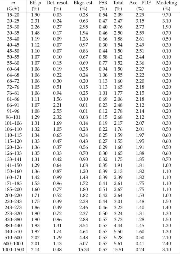
Table 1: Summary of the systematic uncertainties for the dimuon channel dσ/dm measure-ment. The “Total” is a quadratic sum of all sources except for the Acc.+PDF and Modeling.

m Eff. ρ Det. resol. Bkgr. est. FSR Total Acc.+PDF Modeling

(GeV) (%) (%) (%) (%) (%) (%) (%) 15–20 1.90 0.03 0.28 0.54 2.09 2.29 9.70 20–25 2.31 0.24 0.63 0.47 2.47 3.15 3.10 25–30 2.26 0.27 2.95 0.40 3.76 2.73 1.90 30–35 1.48 0.17 1.94 0.46 2.50 2.59 0.70 35–40 1.19 0.09 1.26 0.66 1.88 2.61 0.50 40–45 1.12 0.07 0.97 0.30 1.54 2.49 0.30 45–50 1.10 0.07 0.86 0.44 1.50 2.51 0.10 50–55 1.07 0.10 0.67 0.58 1.42 2.44 0.10 55–60 1.07 0.15 0.69 0.77 1.52 2.36 0.20 60–64 1.06 0.19 0.35 0.94 1.50 2.27 0.20 64–68 1.06 0.22 0.24 1.06 1.55 2.22 0.30 68–72 1.06 0.30 0.20 1.13 1.60 2.20 0.20 72–76 1.05 0.51 0.15 1.13 1.65 2.18 0.20 76–81 1.06 0.94 0.25 1.01 1.77 2.15 0.20 81–86 1.11 1.56 0.10 0.69 2.06 2.18 0.10 86–91 1.07 2.21 0.01 0.23 2.48 2.12 0.20 91–96 1.08 2.55 0.01 0.12 2.78 2.14 0.20 96–101 1.29 2.32 0.08 0.15 2.68 2.12 0.30 101–106 1.31 1.69 0.14 0.19 2.17 2.07 0.30 106–110 1.32 1.05 0.28 0.22 1.76 2.01 0.50 110–115 1.34 0.65 0.34 0.25 1.59 1.97 0.60 115–120 1.33 0.47 0.43 0.27 1.55 1.95 0.60 120–126 1.36 0.37 0.56 0.29 1.60 1.91 0.50 126–133 1.35 0.33 0.70 0.30 1.65 1.88 0.60 133–141 1.31 0.42 0.90 0.32 1.75 1.85 0.70 141–150 1.29 0.64 1.08 0.35 1.91 1.81 1.00 150–160 1.36 0.87 1.20 0.39 2.13 1.82 1.10 160–171 1.42 0.99 1.48 0.39 2.39 1.82 1.10 171–185 1.53 0.96 1.72 0.41 2.61 1.75 1.10 185–200 1.60 0.77 1.80 0.51 2.67 1.75 1.10 200–220 1.71 0.52 1.82 0.42 2.64 1.53 1.00 220–243 1.75 0.39 2.28 0.44 3.01 1.48 1.50 243–273 1.86 0.49 2.46 0.46 3.23 1.40 1.40 273–320 1.90 0.72 2.37 0.50 3.24 1.31 1.30 320–380 1.90 0.96 2.88 0.57 3.73 1.28 1.50 380–440 1.93 1.31 3.54 0.57 4.44 1.45 1.20 440–510 1.97 1.74 4.64 0.57 5.50 1.60 1.30 510–600 2.02 1.79 4.48 0.57 5.28 0.50 2.10 600–1000 2.01 1.13 5.07 0.57 5.61 0.41 2.40 1000–1500 2.14 0.48 15.34 0.57 15.51 0.24 3.10

Table 2: Summary of the systematic uncertainties for the dielectron channel dσ/dm measure-ment. E-scale indicates the energy scale uncertainty. The “Total” is a quadratic sum of all sources except for the Acc.+PDF and Modeling.

m E-scale Eff. ρ Det. resol. Bkgr. est. Total Acc.+PDF Modeling

(GeV) (%) (%) (%) (%) (%) (%) (%) 15–20 1.4 3.0 1.9 0.3 3.8 3.0 9.7 20–25 2.5 2.3 3.3 0.7 4.8 2.2 3.1 25–30 1.5 2.7 1.9 1.1 3.8 2.2 1.9 30–35 1.4 3.2 1.4 4.4 5.8 2.2 0.7 35–40 0.6 2.3 1.1 5.5 6.1 2.1 0.5 40–45 0.7 1.8 1.1 7.1 7.4 2.0 0.3 45–50 0.7 1.5 1.3 8.9 9.1 2.0 0.1 50–55 3.3 1.2 1.7 3.4 5.2 2.0 0.1 55–60 2.8 1.0 2.4 2.5 4.5 2.0 0.2 60–64 6.4 0.9 3.8 2.7 8.0 1.9 0.2 64–68 2.4 0.9 4.9 2.4 6.0 1.9 0.3 68–72 2.1 0.9 5.2 1.8 5.9 1.9 0.2 72–76 1.5 0.8 5.3 1.2 5.7 1.8 0.2 76–81 2.0 0.8 3.7 0.5 4.4 1.8 0.2 81–86 5.9 0.8 2.3 0.2 6.4 1.7 0.1 86–91 8.8 0.7 0.7 0.1 8.8 1.7 0.2 91–96 8.4 0.7 0.7 0.0 8.4 1.7 0.2 96–101 15.6 0.7 3.7 0.2 16.1 1.7 0.3 101–106 17.6 0.8 5.8 0.4 18.6 1.7 0.3 106–110 10.4 0.9 13.1 1.0 16.7 1.7 0.5 110–115 5.5 0.9 10.2 1.2 11.6 1.6 0.6 115–120 2.5 1.0 10.2 1.6 10.7 1.6 0.6 120–126 2.0 1.1 8.1 1.9 8.6 1.6 0.5 126–133 2.9 1.2 6.0 2.1 7.1 1.6 0.6 133–141 4.9 1.2 4.7 2.1 7.2 1.6 0.7 141–150 3.3 1.3 4.7 2.7 6.5 1.6 1.0 150–160 3.5 1.4 4.9 3.1 6.9 1.6 1.1 160–171 6.7 1.5 3.9 2.6 8.3 1.7 1.1 171–185 5.6 1.6 4.1 3.6 8.0 1.6 1.1 185–200 4.1 1.6 3.8 3.4 6.7 1.7 1.1 200–220 2.6 1.7 2.9 3.1 5.3 1.6 1.0 220–243 1.8 1.9 3.3 3.9 5.7 1.7 1.5 243–273 1.6 2.0 3.4 4.0 5.9 1.7 1.4 273–320 1.1 2.1 3.0 4.4 5.9 1.7 1.3 320–380 1.8 2.5 3.7 4.2 6.4 1.9 1.5 380–440 3.3 3.2 5.8 5.8 9.4 2.3 1.2 440–510 3.2 3.8 5.3 5.0 8.8 2.8 1.3 510–600 3.4 1.3 1.2 3.8 5.4 0.6 2.1 600–1000 1.5 1.3 2.2 7.1 7.7 0.5 2.4 1000–1500 7.8 0.9 1.3 33.3 34.2 0.4 3.1

4.7 Systematic uncertainties 21

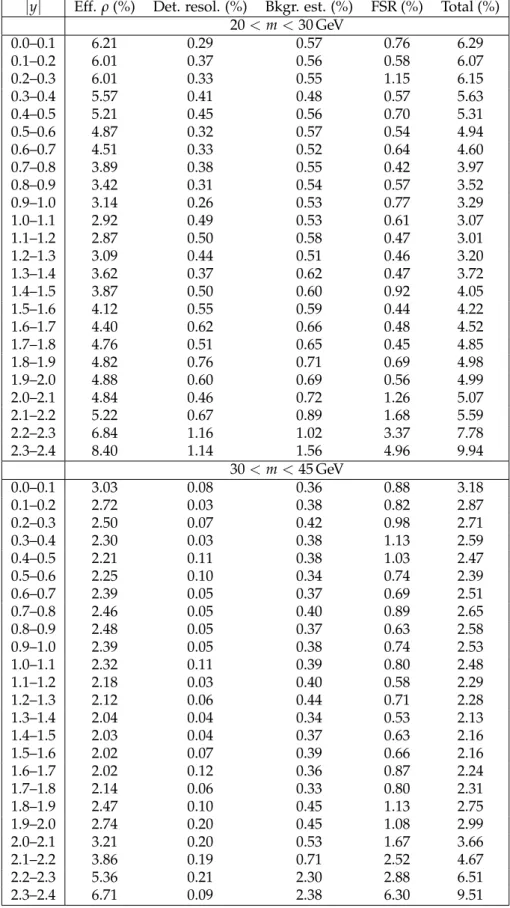
Table 3: Summary of systematic uncertainties in the dimuon channel for 20<m<30 GeV and 30<m<45 GeV bins as a function of|y|. The “Total” is a quadratic sum of all sources.

|y| Eff. ρ (%) Det. resol. (%) Bkgr. est. (%) FSR (%) Total (%) 20<m<30 GeV 0.0–0.1 6.21 0.29 0.57 0.76 6.29 0.1–0.2 6.01 0.37 0.56 0.58 6.07 0.2–0.3 6.01 0.33 0.55 1.15 6.15 0.3–0.4 5.57 0.41 0.48 0.57 5.63 0.4–0.5 5.21 0.45 0.56 0.70 5.31 0.5–0.6 4.87 0.32 0.57 0.54 4.94 0.6–0.7 4.51 0.33 0.52 0.64 4.60 0.7–0.8 3.89 0.38 0.55 0.42 3.97 0.8–0.9 3.42 0.31 0.54 0.57 3.52 0.9–1.0 3.14 0.26 0.53 0.77 3.29 1.0–1.1 2.92 0.49 0.53 0.61 3.07 1.1–1.2 2.87 0.50 0.58 0.47 3.01 1.2–1.3 3.09 0.44 0.51 0.46 3.20 1.3–1.4 3.62 0.37 0.62 0.47 3.72 1.4–1.5 3.87 0.50 0.60 0.92 4.05 1.5–1.6 4.12 0.55 0.59 0.44 4.22 1.6–1.7 4.40 0.62 0.66 0.48 4.52 1.7–1.8 4.76 0.51 0.65 0.45 4.85 1.8–1.9 4.82 0.76 0.71 0.69 4.98 1.9–2.0 4.88 0.60 0.69 0.56 4.99 2.0–2.1 4.84 0.46 0.72 1.26 5.07 2.1–2.2 5.22 0.67 0.89 1.68 5.59 2.2–2.3 6.84 1.16 1.02 3.37 7.78 2.3–2.4 8.40 1.14 1.56 4.96 9.94 30<m<45 GeV 0.0–0.1 3.03 0.08 0.36 0.88 3.18 0.1–0.2 2.72 0.03 0.38 0.82 2.87 0.2–0.3 2.50 0.07 0.42 0.98 2.71 0.3–0.4 2.30 0.03 0.38 1.13 2.59 0.4–0.5 2.21 0.11 0.38 1.03 2.47 0.5–0.6 2.25 0.10 0.34 0.74 2.39 0.6–0.7 2.39 0.05 0.37 0.69 2.51 0.7–0.8 2.46 0.05 0.40 0.89 2.65 0.8–0.9 2.48 0.05 0.37 0.63 2.58 0.9–1.0 2.39 0.05 0.38 0.74 2.53 1.0–1.1 2.32 0.11 0.39 0.80 2.48 1.1–1.2 2.18 0.03 0.40 0.58 2.29 1.2–1.3 2.12 0.06 0.44 0.71 2.28 1.3–1.4 2.04 0.04 0.34 0.53 2.13 1.4–1.5 2.03 0.04 0.37 0.63 2.16 1.5–1.6 2.02 0.07 0.39 0.66 2.16 1.6–1.7 2.02 0.12 0.36 0.87 2.24 1.7–1.8 2.14 0.06 0.33 0.80 2.31 1.8–1.9 2.47 0.10 0.45 1.13 2.75 1.9–2.0 2.74 0.20 0.45 1.08 2.99 2.0–2.1 3.21 0.20 0.53 1.67 3.66 2.1–2.2 3.86 0.19 0.71 2.52 4.67 2.2–2.3 5.36 0.21 2.30 2.88 6.51 2.3–2.4 6.71 0.09 2.38 6.30 9.51

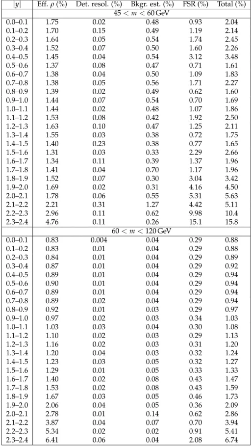
Table 4: Summary of systematic uncertainties in the dimuon channel for 45<m<60 GeV and 60<m<120 GeV bins as a function of|y|. The “Total” is a quadratic sum of all sources.

|y| Eff. ρ (%) Det. resol. (%) Bkgr. est. (%) FSR (%) Total (%) 45<m<60 GeV 0.0–0.1 1.75 0.02 0.48 0.93 2.04 0.1–0.2 1.70 0.15 0.49 1.19 2.14 0.2–0.3 1.64 0.05 0.54 1.74 2.45 0.3–0.4 1.52 0.07 0.50 1.60 2.26 0.4–0.5 1.45 0.04 0.54 3.12 3.48 0.5–0.6 1.37 0.08 0.47 0.71 1.61 0.6–0.7 1.38 0.04 0.50 1.09 1.83 0.7–0.8 1.38 0.05 0.56 1.71 2.27 0.8–0.9 1.39 0.02 0.49 0.62 1.60 0.9–1.0 1.44 0.07 0.54 0.70 1.69 1.0–1.1 1.44 0.02 0.48 1.07 1.86 1.1–1.2 1.53 0.08 0.42 1.92 2.50 1.2–1.3 1.63 0.10 0.47 1.25 2.11 1.3–1.4 1.55 0.03 0.38 0.72 1.75 1.4–1.5 1.40 0.23 0.38 0.77 1.65 1.5–1.6 1.31 0.03 0.33 2.29 2.66 1.6–1.7 1.34 0.11 0.39 1.37 1.96 1.7–1.8 1.41 0.04 0.70 1.17 1.96 1.8–1.9 1.52 0.07 0.30 3.04 3.42 1.9–2.0 1.69 0.02 0.31 4.16 4.50 2.0–2.1 1.78 0.06 0.55 5.31 5.63 2.1–2.2 2.21 0.31 1.27 4.42 5.11 2.2–2.3 2.96 0.11 0.62 9.98 10.4 2.3–2.4 4.76 0.11 0.26 15.1 15.8 60<m<120 GeV 0.0–0.1 0.83 0.004 0.04 0.29 0.88 0.1–0.2 0.83 0.01 0.04 0.29 0.88 0.2–0.3 0.84 0.01 0.04 0.29 0.89 0.3–0.4 0.87 0.01 0.04 0.29 0.92 0.4–0.5 0.89 0.01 0.04 0.29 0.94 0.5–0.6 0.90 0.01 0.04 0.29 0.94 0.6–0.7 0.89 0.01 0.04 0.29 0.94 0.7–0.8 0.89 0.02 0.04 0.29 0.94 0.8–0.9 0.92 0.01 0.03 0.29 0.97 0.9–1.0 0.97 0.02 0.03 0.34 1.03 1.0–1.1 1.03 0.03 0.04 0.30 1.08 1.1–1.2 1.10 0.02 0.03 0.29 1.13 1.2–1.3 1.16 0.02 0.03 0.31 1.20 1.3–1.4 1.20 0.04 0.03 0.32 1.24 1.4–1.5 1.23 0.03 0.05 0.32 1.27 1.5–1.6 1.29 0.01 0.05 0.33 1.33 1.6–1.7 1.40 0.02 0.08 0.43 1.47 1.7–1.8 1.53 0.02 0.08 0.43 1.59 1.8–1.9 1.67 0.03 0.05 0.46 1.73 1.9–2.0 2.06 0.04 0.05 0.36 2.09 2.0–2.1 2.78 0.01 0.14 0.62 2.86 2.1–2.2 3.87 0.04 0.07 0.70 3.94 2.2–2.3 5.34 0.02 0.02 0.91 5.41 2.3–2.4 6.41 0.06 0.04 2.08 6.74

4.7 Systematic uncertainties 23

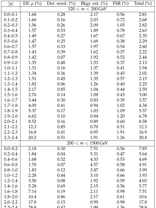
Table 5: Summary of systematic uncertainties in the dimuon channel for 120 < m < 200 GeV and 200<m<1500 GeV bins as a function of|y|. The “Total” is a quadratic sum of all sources.

|y| Eff. ρ (%) Det. resol. (%) Bkgr. est. (%) FSR (%) Total (%) 120<m<200 GeV 0.0–0.1 1.68 0.28 2.17 0.56 2.81 0.1–0.2 1.60 0.16 2.03 0.72 2.68 0.2–0.3 1.56 0.26 2.09 1.05 2.82 0.3–0.4 1.57 0.53 1.89 0.78 2.63 0.4–0.5 1.49 0.27 1.67 0.67 2.35 0.5–0.6 1.47 0.25 1.69 0.38 2.29 0.6–0.7 1.57 0.33 1.97 0.54 2.60 0.7–0.8 1.43 0.39 1.62 0.37 2.22 0.8–0.9 1.42 0.07 1.92 0.52 2.44 0.9–1.0 1.35 0.48 1.53 0.37 2.13 1.0–1.1 1.31 0.16 1.37 0.41 1.94 1.1–1.2 1.34 0.36 1.39 0.45 2.02 1.2–1.3 1.51 0.45 1.35 0.57 2.15 1.3–1.4 1.82 0.06 1.26 0.40 2.25 1.4–1.5 2.17 0.85 1.04 0.44 2.59 1.5–1.6 2.76 0.14 1.08 0.43 3.00 1.6–1.7 3.44 0.30 0.83 0.39 3.57 1.7–1.8 4.09 0.41 0.94 1.02 4.34 1.8–1.9 5.37 0.17 1.03 1.09 5.57 1.9–2.0 6.62 0.10 0.84 1.20 6.78 2.0–2.1 8.52 0.16 0.89 0.60 8.58 2.1–2.2 12.3 0.85 0.70 0.51 12.3 2.2–2.3 16.8 0.41 0.95 1.91 16.9 2.3–2.4 20.2 0.51 1.91 1.26 20.4 200<m<1500 GeV 0.0–0.2 2.18 0.30 7.51 0.56 7.85 0.2–0.4 1.84 0.04 5.31 0.47 5.64 0.4–0.6 1.68 0.32 4.33 0.53 4.69 0.6–0.8 1.70 0.07 4.57 0.58 4.91 0.8–1.0 1.83 0.12 3.47 0.66 3.99 1.0–1.2 2.28 0.44 3.10 0.66 3.93 1.2–1.4 3.50 0.08 1.92 0.59 4.03 1.4–1.6 5.28 0.65 2.15 0.56 5.77 1.6–1.8 7.14 0.19 2.11 0.98 7.51 1.8–2.0 10.4 0.86 2.17 0.61 10.6 2.0–2.2 17.8 0.15 0.99 0.98 17.8 2.2–2.4 28.8 0.42 1.99 1.36 28.9