Universidade Nova de Lisboa - ISEGI Lisboa, Portugal
S
S
A
A
K
K
W
W
e
e
b
b
©
©
A thesis submitted in partial satisfaction of the requirements for the degree of Doctor of Philosophy in Information Systems
by
João Garrott Marques Negreiros
Chairperson: Marco Painho, Ph.D.
Copyright © by
João Garrott Marques Negreiros All Rights Reserved
ABSTRACT
SAKWeb©
by
João Garrott Marques Negreiros
The present research focuses on the first software to offer spatial autocorrelation and association measures, spatial exploratory tools, variography and Ordinary Kriging (OK) in the World Wide Web. Exploiting IE®, ASP®, PHP® and IIS® capabilities, SAKWeb© version 2.0 was designed in an attractive and straightforward way for everyone’s use. Major commercial off-the-shelf spatial software is reviewed to confirm SAKWeb© improvements. As confirmed by Green and Bossomaier [2002], “it is essential for geographical studies to provide basic spatial autocorrelation indices and significance test computer programs for personal computers”.
Spatial autocorrelation can provide an Exploratory Spatial Data Analysis (ESDA) tool for atypical locations, trends, transition regions and spatial patterns. The weight matrix (W) is assessed on the basis of the covariogram contiguity. In accordance with various distance ranges, SAKWeb© selects the one with the highest global Moran I to setup the conventional and the Moran location scatterplot. In addition, the Moran I correlogram may lead to a re-estimation process of the best variogram range, sill, model and nugget-effect factors. Some of the possibilities are dropping outliers, tracing patterns of quadrants I and III, highlighting transition samples or maintaining the original dataset. IDW is also stressed as a poor method for W specification. Nearest neighborhood analysis and brushing operations are added features for enhanced dataset familiarity.
SAKWeb© presents the Moran variance scatterplot because the conventional one is not sensitive to neighborhood variance. The 2D view stresses outliers and stable and unpredictable regions. It can also be used with trend residuals to reveal heteroskedasticity.
The Web driven interface using hypermedia help with sound and movement is also provided in an e-Learning structure that includes an IRC, Email and News service, to close the knowledge gap between experts and common GIS users. This requirement results from two spatial autocorrelation and Kriging knowledge surveys which were carried out in several prestigious Portuguese institutions, and revealed a vast lack of awareness of both issues.
The SAKWeb© approach regarding the nugget-effect is significant. Four strategies are presented:
• γ(0)=0;
• γ(0)=0 but including C0 for distances greater than zero;
• γ(0) division into two scales: γ1(0)=0 and γ1(0<h1<=Shortest Sampling
Interval)=the Spherical, Exponential or Gaussian model whose sill equals the second long range structure, γ2(h), at SSI lag distance;
• If measurement error is given then this factor will be included in the Kriging system but it will lead to a non-exact Kriging version.
“The variogram sill does not reflect the true global variance, which is generally lower, because the variogram function poorly describes the short scale variability” [Isaaks, Srivastava, 1989]. Thus, if the estimated global mean (EGM) and the estimated global variance (EGV) indices are assessed on the basis of the nearest neighbor analysis then a sill rescaling operation is possible for OK variance and region confidence interval enhancement (both local and global). A new classical local spatial variance index that is both data and geometry dependent is introduced. The assessment of combined Kriging estimates weighted by the OK variance is also accomplished. The Colorado (USA) grasshopper datasets of 1993, 1994, 1995 and 1997 are also analyzed and presented by SAKWeb© with remarkable conclusions between the Moran I correlogram and the variogram parameters.
RESUMO DA DISSERTAÇÂO
SAKWeb©
por
João Garrott Marques Negreiros
A presente investigação introduz o primeiro geosoftware Web relativo a medidas de autocorrelação espacial e associação, ferramentas de análise exploratória de dados, variografia e Krigagem ordinária. Através do IE®, ASP®, PHP® e IIS®, o SAKWeb© versão 2.0 foi desenvolvido de um modo atractivo e directo para todo o tipo de utilizadores. Assim, a maior parte dos geosoftwares comerciais foram re-analisados de modo a confirmar a sua inovação e presente desenvolvimento. Confirmado por Green e Bossomaier [2002], “é essencial nos estudos geográficos providenciar software relacionado com os indices básicos de autocorrelação espacial”.
A autocorrelação espacial permite fornecer um conjunto de ferramentas exploratórias para dados espaciais sobre a localização de observações atipicas, a tendencia geral da distribuição espacial, as regiões de transição e os padrões espaciais. A matriz de pesos (W) é calculado com base na contiguidade do covariograma. De acordo com várias distancias, o SAKWeb© seleciona a amplitude baseado no valor mais alto indicado pelo Moran I e que servirá de base ao Moran Scatterplot convencional e de localização. Uma outra vantagem deste método iterativo é a sua capacidade de indicar pistas sobre os parâmetros principais do variograma (modelo, efeito de pepita, amplitude e patamar) num processo de re-estimação. Rejeitar outliers, detectar os padrões do I e III quadrante, emfatizar as observações localizadas em regiões de transição ou manter o conjunto das amostras iniciais são algumas das possibilidades. O método IDW é indicado como um método pobre e ineficaz na especificação da matriz W. Igualmente, a análise de índices de vizinhança mais próxima e operacões de sub-selecção de amostras em tempo real são caracteristicas enaltecidas pelo SAKWeb©.
SAKWeb© estabelece uma nova ferramenta, a variância do Moran Scatterplot, pois a tradicional não é sensível ao segundo momento de uma distribuição. A sua visão 2D sublinha ‘outliers’, regiões estacionárias e areas instáveis podendo também este ser utilizado para testemunhar a variância dos resíduos resultantes de uma operação de “detrend”.
A interface Web usando hipermédia no seu menu de Help numa estrutura de e-Learning incluindo IRC e serviço de News é também importante. De facto, os resultados dos inquéritos sobre geoestatistica realizado em várias instituições prestigiadas Portuguesas revelou uma grande falta de conhecimentos e sensibilidade associado a este assunto.
A metodologia associado ao SAKWeb© relativo ao efeito de pepita é significante. Quatro estratégias são apresentadas:
• γ(0)=0;
• γ(0)=0 mas incluindo o efeito de pepita para distancias maiores que zero; • γ(0) é dividido em duas estruturas embricadas: γ1(0)=0 e γ1(0<h1<=Distancia
Minima Amostral)=Esférico, Exponencial ou Gaussiano cujo patamar é igual à segunda macro-estrutura, γ2(h), na distancia DMA;
• Se o erro de amostragem for considerado então este factor é incluido no sistema linear de Krigagem mas originando uma versão de interpolador não exacta.
“O patamar do variograma não reflecte a variância global das observações, geralmente mais baixa, porque o variograma descreve pobremente a variabilidade local” [Isaaks e Srivastava, 1989]. Assim, a média e a variância global estimada pela análise da vizinhaça mais próxima é calculado. Numa operação de re-escalonamento do patamar é possivel aperfeiçoar a variância da Krigagem ordinária e do intervalo da região de confiança. Um novo índice de incerteza, the spatial local classical variance, baseado na dependência geométrica e valores das amostras é desenvolvido. Finalmente, quatro conjunto de observações de pragas de gafanhotos no estado do Colorado, USA, é analisado pelo SAKWeb© com algumas conclusões notáveis.
RÉSUMÉ ANALYTIQUE
SAKWeb©
par
João Garrott Marques Negreiros
La recherche présentée ici traite du premier logiciel Web appliqué à la géographie qui a pour objet les mesures d’autocorrélation spatiale et d’association, les outils d’analyse exploratoire de données, la variographie et le Kriging ordinaire (OK). Au moyen de l’IE®, ASP®, PHP® and IIS®, la version 2.0 du SAKWeb© a été élaborée d’une manière attrayante et directe pour tout type d’utilisateurs. Ainsi, la majeure partie des logiciels destinés aux géographes et disponibles dans le commerce a été ré-examinée afin de pouvoir confirmer le caractère innovateur du logiciel SAKWeb© et son développement actuel. Comme cela a été confirmé par Green and Bossomaier [2002], “il est indispensable pour les études géographiques de disposer d’un programme traitant des indices de base d’autocorrélation spatiale”.
L’autocorrélation spatiale permet de fournir un ensemble d’outils d’investigation de données spatiales au sujet de la localisation d’observations atypiques, des tendances générales de la distribution spatiale, des régions de transition et des modèles spatiaux. La matrice de poids (W) est évaluée sur base de la contiguïté du co-variogramme. En fonction des diverses distances, le SAKWeb© sélectionne l’amplitude en se basant sur la valeur la plus haute indiquée par le Moran I et qui servira de base au Scatterplot Moran conventionnel ainsi que de localisation. Un autre avantage de cette méthode répétitive est sa capacité d’indiquer des pistes au sujet des paramètres principaux du variogramme (modèle, effet de pépite, amplitude et seuil) dans un processus de ré-évaluation. Le rejet des observations aberrantes (outliers), la détection des modèles de quadrant I et III, la mise en évidence des observations localisées dans des régions de transition ou le maintien de l’ensemble des échantillons initiaux sont quelques-unes de possibilités qu’offre le SAKWeb©. La méthode IDW est considérée comme étant limitée et inefficace pour la spécification de la matrice W. De même, l’analyse des indices de voisinage
le plus proche et les opérations de sous-sélection des échantillons en temps réel sont des caractéristiques supplémentaires du SAKWeb©.
Le SAKWeb© crée un nouvel outil, la variance du scatterplot Moran parce que le scatterplot conventionnel ne réagit pas aux variations de voisinage au second moment d’une distribution. La vision 2D du SAKWeb© met en évidence les observations aberrantes (outliers) ainsi que les régions stationnaires et les aires instables. Elle peut aussi être utilisée pour prouver la variation des éléments résiduels résultant d’une opération de ‘detrend’.
L’interface de réseau (web) est aussi importante. Elle utilise l’hypermédia dans son menu Aide incorporé dans une structure d’apprentissage électronique (e-Learning) comprenant un IRC et un service de News. En fait, les résultats des enquêtes sur la géostatistique réalisées dans diverses institutions portugaises prestigieuses ont révélé un important manque de connaissances et de sensibilisation à ce sujet.
La méthodologie associée au SAKWeb© en ce qui concerne l’effet de pépite est importante. Quatre stratégies sont présentées:
• γ(0)=0;
• γ(0)=0 mais comprenant l’effet de pépite pour des distances supérieures à
zéro;
• γ(0) est divisé en deux échelles reliées entre elles: γ1(0)=0 et
γ1(0<h1<=distance d’échantillonage la plus courte, SSI)=Sphérique,
Exponentielle ou du modèle de Gauss dont le seuil est égal à la seconde macrostructure, γ2(h), à distance SSI (valeur de la force du signal);
• Si l’erreur d’échantillonage est prise en compte, alors ce facteur est inclus dans le système linéaire du Kriging mais cela créera une version inexacte d’interpolateur.
“Le seuil du variogramme ne reflète pas la véritable variance globale des observations, qui est généralement inférieure, parce que le variogramme décrit mal la variabilité locale” [Isaaks, Srivastava, 1989]. Ainsi sont calculées la moyenne globale estimée et la variance globale estimée sur base de l’analyse de voisinage la
plus proche. Par une opération de ré-échelonnement du seuil, il est possible de perfectionner la variance de l’opération de Kriging ordinaire et de l’intervalle de la région de confiance. Ainsi est développé un nouvel indice d’incertidude, la variance spatiale locale classique, qui est basé sur la dépendance géométrique et les valeurs des échantillons. Enfin, quatre ensembles d’observations d’invasions de sauterelles dans l’état du Colorado (États-Unis) sont analysés par le SAKWeb© et ont conduit à quelques conclusions remarquables.
ACKNOWLEDEGMENTS
This document represents the culmination of a process which required a tremendous amount of dedication, not only from the author but also from a number of people who assisted in producing it in countless ways. In recognition of his unflagging enthusiasm and constant encouragement, I would like to thank Professor Marco Painho, Ph.D., chairperson of my thesis committee, and my advisor, for his knowledgeable guidance during the course of my doctoral studies at ISEGI, Universidade Nova de Lisboa. I would like to extend my appreciation to Professor Jorge de Sousa, Ph.D., from IST, Universidade Técnica de Lisboa, for leading me to this motivating research field and to give special thanks to Professor Pedro Coelho, Ph.D., for his helpful statistical suggestions. The kind support provided by ISEGI, in particular Dr. Francisco Marques, and CIIST computer center and Professor Pierre Goovaerts, Professor Ana Costa and Professor Fernando Bação’s criticism are gratefully acknowledged. Thanks to Professor Archie Collins for the English review. I am also grateful to my parents who believed in my ability to get a Ph.D. long before I did. Finally, I would like to thank my eternal irreplaceable friend Paulo Pereira for his valuable Web graphics help and my wife Claudia for clearing my brain of the dust accumulated by spending too many hours behind a computer screen. Certainly, I could not forget my son Daniel for waking me up every night for a diaper change while Dad finished school. This endeavor is dedicated to them.
The research presented in this thesis was partially funded and supported by
“The emphasis is on where, the jurisdiction of spatial statistics.”
J. Berry
“What makes spatial statistics different from statistics? Lots and lots of computer programming.”
Unknown author
I am sorry for this lengthy thesis but I did not have the time to write a smaller one.
TABLE OF CONTENTS
1. Introduction _________________________________________________ 27
1.1. Statement of the Problem_______________________________________ 27
1.2. Research Objectives ___________________________________________ 32
1.3. Constraints and Limitations ____________________________________ 34
1.4. Hypothesis ___________________________________________________ 35
1.5. Methodology _________________________________________________ 35
1.5.1. Spatial Analysis: The Missing Data Issue________________________________ 37 1.5.2. Spatial Analysis: Interpolation, Implementation Review and Software Evaluation 38 1.5.3. Spatial Analysis: User Know-how _____________________________________ 40 1.5.4. SAKWeb©________________________________________________________ 40
1.6. Relevance____________________________________________________ 42
1.7. Organization _________________________________________________ 47
2. Spatial Analysis: The Missing Data Issue _________________________ 49
2.1. Geography and Geographical Data _______________________________ 49
2.2. GIS and Spatial Analysis: An Overview ___________________________ 52
2.3. Spatial Autocorrelation ________________________________________ 56
2.4. Visualizing What Is Not Observed _______________________________ 62
2.4.1. The Variogram Cloud and the Cressie Box Plot ___________________________ 63 2.4.2. The Spatial Lag Scatterplot ___________________________________________ 64 2.4.3. The Spatial Lag Pies ________________________________________________ 64 2.4.4. The Moran I_______________________________________________________ 65 2.4.5. The Geary C ______________________________________________________ 66 2.4.6. The Local Gi(d) and the Global G(d) ___________________________________ 67
2.4.7. The Local Moran___________________________________________________ 69 2.4.8. The Moran Scatterplot_______________________________________________ 69
2.5. Spatial Autoregression Models __________________________________ 70
2.5.1. Spatial Autoregression: Residuals______________________________________ 72 2.5.1.1. LADS_______________________________________________________ 75
2.5.1.2. Join-Count Statistics ___________________________________________ 76
2.6. Spatial Autocorrelation, Autoregression and Kriging: The Missing Data
Issue 77
2.7. W Matrix: IDW versus Binary Contiguity_________________________ 80
2.7.1. Case Study 1: Appendix I ____________________________________________ 81 2.7.2. Case Study 2: Appendix J ____________________________________________ 84 2.7.3. Discussion ________________________________________________________ 86
2.8. Conclusions__________________________________________________ 89
3. Spatial Analysis: Interpolation _________________________________ 91
3.1. Spatial Deterministic Interpolators_______________________________ 91
3.1.1. Drawing Boundaries and TIN _________________________________________ 91 3.1.2. Global Polynomial Trend ____________________________________________ 92 3.1.3. Fourier ___________________________________________________________ 94 3.1.4. B-Spline__________________________________________________________ 95 3.1.5. Inverse Distance Weighting __________________________________________ 95
3.2. The Nature of Regionalized Data: Introduction ____________________ 97
3.3. Exploratory (A)Spatial Data Analysis ___________________________ 104
3.3.1. Distribution Standardization _________________________________________ 106 3.3.2. Sampling Considerations____________________________________________ 110
3.4. The Variogram ______________________________________________ 112
3.4.1. SAKWeb© Isotropic Variogram Models ________________________________ 119 3.4.2. Computational Variogram Issues _____________________________________ 121
3.5. Ordinary Kriging ____________________________________________ 124
3.5.1. The Cross-Validation Procedure ______________________________________ 126
3.6. Assessing Uncertainty ________________________________________ 127
3.6.1. The Classical Local Spatial Variance __________________________________ 131
3.7. Conclusions_________________________________________________ 135
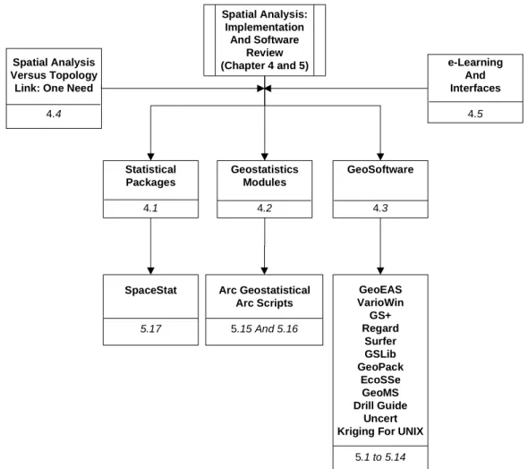
4. Spatial Analysis: Implementation Review _______________________ 137
4.1. Statistical Packages __________________________________________ 137
4.2. GIS Modules ________________________________________________ 140
4.3. Independent GeoSoftware _____________________________________ 142
4.5. e-Learning and Interfaces _____________________________________ 146
4.6. Conclusions _________________________________________________ 149
5. Spatial Analysis: Software Evaluation __________________________ 151
5.1. Surface III®_________________________________________________ 151 5.2. VarioWin®__________________________________________________ 152 5.3. GS+® ______________________________________________________ 153 5.4. GeoMS®____________________________________________________ 154 5.5. REGARD®__________________________________________________ 155 5.6. GMS®______________________________________________________ 157 5.7. GSLib® and GsTL®___________________________________________ 158
5.8. Kriging For Berkley Unix®_____________________________________ 159
5.9. Uncert® ____________________________________________________ 160
5.10. GEO-EAS® _________________________________________________ 161
5.11. Surfer®_____________________________________________________ 162
5.12. EcoSSe®____________________________________________________ 163
5.13. GeoPack®___________________________________________________ 164
5.14. ArcGIS Geostatistical Analyst® Module __________________________ 164
5.15. Kriging ArcScripts®__________________________________________ 166
5.16. SpaceStat®__________________________________________________ 167
5.17. Conclusions _________________________________________________ 171
6. Spatial Analysis: User Know-how ______________________________ 173
6.1. Modest Expertise in Sophisticated Spatial Analysis_________________ 173 6.2. Statistical and Geographical Knowledge: The Perfect Marriage ______ 178
6.3. Spatial Autocorrelation and Kriging: The Web Solution ____________ 180
6.4. Conclusions _________________________________________________ 188
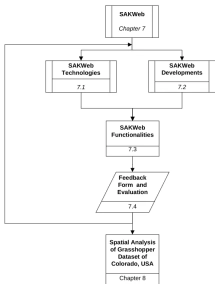
7. SAKWeb©__________________________________________________ 189
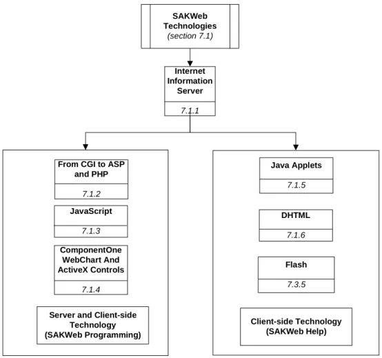
7.1. SAKWeb© Technologies _______________________________________ 192
7.1.2. From CGI to ASP® and PHP®________________________________________ 195 7.1.3. JavaScript® ______________________________________________________ 200 7.1.4. ActiveX® and Component One WebChart®_____________________________ 202 7.1.5. Java Applets® ____________________________________________________ 208 7.1.6. DHTML_________________________________________________________ 211
7.2. SAKWeb© Developments______________________________________ 212
7.2.1. The SAKWeb© Variogram - Moran I - Moran Scatterplot Optimal ESDA _____ 212 7.2.1.1. Case Study: The San Diego Dataset ______________________________ 213 7.2.1.2. Case Study: The Africa Dataset__________________________________ 214 7.2.1.3. Log Transformation Impact on Moran I ___________________________ 215 7.2.1.4. Moran I as a Scale Pattern Factor for the Moran Scatterplot____________ 216 7.2.1.5. The Issue of True and False Outliers ______________________________ 219 7.2.1.6. The Undercover Uncertainty Region of the Conventional Moran Scatterplot 221
7.2.1.7. The SAKWeb© Moran Location Scatterplot ________________________ 223 7.2.2. The SAKWeb© Moran Variance Scatterplot ESDA _______________________ 228 7.2.2.1. Case Study: The San Diego Dataset ______________________________ 231 7.2.2.2. Case Study: The GeoEAS® Lead Dataset __________________________ 232 7.2.2.3. Case Study: The Organic Dataset for the Soil in Nebraska _____________ 233 7.2.3. SAKWeb© Variogram Sill Rescaling __________________________________ 235 7.2.3.1. Case Study: The San Diego Dataset ______________________________ 238 7.2.3.2. Case Study: The Africa Dataset__________________________________ 238 7.2.3.3. SAKWeb© Global Confidence Interval ____________________________ 239 7.2.3.4. SAKWeb© Local Confidence Interval_____________________________ 241 7.2.4. SAKWeb© Nugget-effect ___________________________________________ 243 7.2.4.1. Case Study: The GS+® Pb Dataset _______________________________ 252 7.2.4.2. Case Study: The San Diego Dataset ______________________________ 254
7.3. SAKWeb© Functionalities _____________________________________ 255
7.3.1. Data Input and Exploring View_______________________________________ 257 7.3.2. Variography and Spatial Autocorrelation _______________________________ 264 7.3.3. SAKWeb© (Ordinary) Kriging _______________________________________ 268 7.3.4. SAKWeb© Help___________________________________________________ 275
7.4. SAKWeb© End-User Evaluation ________________________________ 282
7.5. Conclusion _________________________________________________ 287
8. SAKWeb©: Spatial Analysis of the Grasshopper in Colorado, USA __ 289
8.2. The Grasshopper Prediction Issue ______________________________ 293
8.3. The Grasshopper Study Region_________________________________ 294
8.4. SAKWeb© Exploratory Data Analysis ___________________________ 296
8.5. SAKWeb© Spatial Autocorrelation ______________________________ 300
8.6. SAKWeb© Variography _______________________________________ 303
8.7. The SAKWeb© Moran Location Scatterplot and Moran Variance
Scatterplot ________________________________________________________ 307
8.8. SAKWeb© Ordinary Kriging ___________________________________ 315
8.9. SAKWeb© Validation Procedures _______________________________ 321
8.10. Conclusion __________________________________________________ 328
9. Summary and General Conclusion _____________________________ 331
9.1. Summary ___________________________________________________ 332
9.2. Discussion of the Hyphoteses ___________________________________ 334
9.3. Limitations and Future Research _______________________________ 337
Literature Cited _________________________________________________ 340 Appendix A_____________________________________________________ 367 Appendix B_____________________________________________________ 373 Appendix C_____________________________________________________ 376 Appendix D_____________________________________________________ 379 Appendix E_____________________________________________________ 380 Appendix F _____________________________________________________ 401 Appendix G ____________________________________________________ 403 Appendix H ____________________________________________________ 406 Appendix I _____________________________________________________ 409 Appendix J _____________________________________________________ 415 Appendix K ____________________________________________________ 419 Appendix L_____________________________________________________ 421
Appendix M____________________________________________________ 423 Appendix N ____________________________________________________ 426 Appendix O ____________________________________________________ 428 Acronyms and Mathematical Symbols ______________________________ 430
LIST OF FIGURES
Figure 1 – The problems in specifying parameters for area objects. _______________________ 30 Figure 2 – The SAKWeb© overall framework. _______________________________________ 36
Figure 3 – The missing data issue and spatial interpolation of SAKWeb©.__________________ 38
Figure 4 – The SAKWeb© organization of spatial analysis implementation review and software evaluation. ____________________________________________________________________ 39
Figure 5 – The overall SAKWeb© development and technical implementation framework. ____ 41
Figure 6 – The SAKWeb© technical implementation view.______________________________ 42
Figure 7 – The SAKWeb© development view.________________________________________ 42
Figure 8 – Population gains and losses on the Portuguese electoral roll at town level. _________ 51 Figure 9 – The spatial lag pies of a Columbus Ohio dataset [Anselin, 1998], where the red bars
indicate neighborhood crime average and the blue ones represent crime in a particular ward. ___ 65
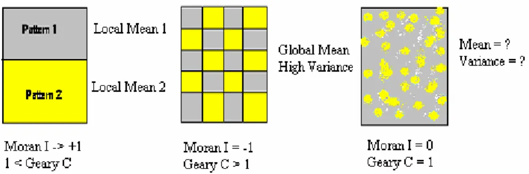
Figure 10 – The Moran I and Geary C measures inferences._____________________________ 67 Figure 11 – Residual plots where the x-axis represents the predicted values while the y-axis is the
associated error [Clark and Hosking, 1986].__________________________________________ 74
Figure 12 – The Moran scatterplot exchanged observation position according to Moran I. _____ 83 Figure 13 – The linear relationships of Moran scatterplots regarding case one and case six. ____ 83 Figure 14 – A comparison of 1/dx contiguities for the impact of weight samples. ____________ 84
Figure 15 – The linear and quadratic polynomial matrices.______________________________ 93 Figure 16 – The variogram and the covariogram function with and without the nugget-effect. _ 102 Figure 17 – The long trend versus short range stationary [Soares, 2000].__________________ 104 Figure 18 – The variogram. _____________________________________________________ 113 Figure 19 - The four type of behavior near the origin._________________________________ 114 Figure 20 – Geometric (left) and geometric with zonal (right) anisotropy. _________________ 118 Figure 21 – An example of the proportional effect [Sousa, 1998]. _______________________ 119 Figure 22 – The spherical model. _________________________________________________ 120 Figure 23 – The exponential model._______________________________________________ 120 Figure 24 – The gaussian model. _________________________________________________ 120 Figure 25 – The setup factors for the variogram construction with regard to the sector binning
method. _____________________________________________________________________ 122
Figure 26 – The Kriging system. _________________________________________________ 125 Figure 27 – The absolute true error against OK variance (left) and local variance (right). _____ 133 Figure 28 – The absolute true error against classical local spatial variance (left) and OK variance
(right). ______________________________________________________________________ 134
Figure 29 – The number of users that use Kriging within GIS modules revealed by the first survey.
____________________________________________________________________________ 141
Figure 30 – The Kriging software awareness revealed by the September 2001 survey. _______ 142 Figure 31 – The XGobi® menu within ArcView®.____________________________________ 144
Figure 32 – The train access time from Lisboa [Figueira, 2000]. ________________________ 145 Figure 33 – The Surface III® data postings. _________________________________________ 151
Figure 34 – The Surface III® search neighborhood.___________________________________ 152
Figure 35 – The Regard® brushing and linking features. _______________________________ 156
Figure 36 – The Regard® brushing and linking features within the scatterplot view. _________ 157
Figure 37 – The Kriging for Berkley Unix® OK interpolation and variance. _______________ 160
Figure 38 – The GEO-EAS® Vario options. ________________________________________ 162
Figure 39 – The Kriging ArcScript® window. _______________________________________ 167
Figure 40 – The SpaceStat® Regress module framework. ______________________________ 169
Figure 41 – The SpaceStat® Extension for ArcView®. ________________________________ 170 Figure 42 – Portuguese GIS users’ acquaintance with spatial interpolation. ________________ 175
Figure 43 – Portuguese GIS users’ knowledge of spatial autocorrelation software. __________ 176 Figure 44 – The high-school teacher’s questionnaire: final answers after fifty hours of five
ArcView® modules. ____________________________________________________________ 178
Figure 45 – User agreement (%) concerning the linkage of spatial autocorrelation and GIS
software. ____________________________________________________________________ 182
Figure 46 – The client-side technology. ____________________________________________ 190 Figure 47 – The server-side technology. ___________________________________________ 190 Figure 48 – The home and authentication page of SAKWeb© that includes the keywords meta tag for search engines robots. _______________________________________________________ 194
Figure 49 – An example of an SSI that returns the date and time of the Web server. _________ 196 Figure 50 – The DOS Commands selection of SAKWeb© including the PHP® code. ________ 199
Figure 51 – Partial view of PHP® configuration. _____________________________________ 200
Figure 52 – The JavaScript® clock output. __________________________________________ 202
Figure 53 – The SAKWeb© main menu. ___________________________________________ 205
Figure 54 – The SAKWeb© trend surface analysis of the GS®+ Pb dataset. ________________ 208
Figure 55 – The independent structure of Java® language. _____________________________ 209
Figure 56 – The general covariogram contiguity plot. _________________________________ 213 Figure 57 – The Moran I correlogram for the San Diego dataset. ________________________ 214 Figure 58 – The Pb dataset results with the Variogram - Moran I - Moran scatterplot optimal
technique. ___________________________________________________________________ 220
Figure 59 – The location samples of the transition regime. _____________________________ 222 Figure 60 – The Pb location samples of the transition regime. __________________________ 222 Figure 61 – The optimal Moran scatterplot flowing chart of SAKWeb©. __________________ 226
Figure 62 – The SAKWeb© view concerning the quadrant I and II of the San Diego dataset. __ 227
Figure 63 – The SAKWeb© view concerning the quadrant III and IV of the San Diego dataset. 228
Figure 64 – The heteroskedasticity question, a problem not resolved by the Moran scatterplot. 229 Figure 65 – The 2D view of the Moran scatterplot extension of Figure 64. ________________ 231 Figure 66 – The Moran variance scatterplot for the San Diego dataset. ___________________ 232 Figure 67 – The Moran variance scatterplot for the GeoEAS® lead dataset. ________________ 233
Figure 68 – The Moran variance scatterplot of the first polynomial residuals for the Nebraska soil
organic dataset. _______________________________________________________________ 235
Figure 69 – The weight assignment methodologies. __________________________________ 236 Figure 70 – The Global Region Confidence Interval option of SAKWeb©, a three step process. 240
Figure 71 – The three step process of the Local Region Confidence Interval option. _________ 243 Figure 72 – The Atkinson [1997] internal and external error view._______________________ 245 Figure 73 – The Kriging interpolation of a Swedish glacier mass with and without the
nugget-effect._______________________________________________________________________ 245
Figure 74 – The three exact nugget-effect approaches of SAKWeb®. ____________________ 247
Figure 75 – OK comparisons between the exact version and the one with all measurement error (1
and 2 represents data locations). __________________________________________________ 248
Figure 76 – The OK system of the working example. _________________________________ 249 Figure 77 – The OK system of the working example, considering with and without measurement
error. _______________________________________________________________________ 249
Figure 78 – Comparison between the exact version of SAKWeb© OK and the one with 30% measurement error. ____________________________________________________________ 251
Figure 79 – The spatial location of the grasshopper densities in 1993 where the dark dots represent
the sites whose OK estimates with a 30% measurement error are lower than the original samples. ____________________________________________________________________________ 252
Figure 80 – The SAKWeb© overall structure. _______________________________________ 257
Figure 81 – The MS-Excel® data input selection. In addition, a movie was added for beginner’s users. _______________________________________________________________________ 258
Figure 82 – The visitor distribution graphic of SAKWeb©. _____________________________ 260
Figure 83 – The local interactive statistics option of SAKWeb©. ________________________ 261
Figure 84 – The 3D scatter view of SAKWeb©. _____________________________________ 263
Figure 85 – The SAKWeb© indicator mapping in a two step process. ____________________ 264
Figure 86 – The SAKWeb© experimental variogram setup. ____________________________ 266
Figure 87 – A partial view of the SAKWeb© variogram fitness process. __________________ 267
Figure 88 – SAKWeb© OK Calculus option. ________________________________________ 269
Figure 89 – Combination of Kriging estimates from OK with C0 (model 1), OK without C0 (model
2) and with two structures (model 3) for the grasshopper 1993 dataset. This includes differences with other SAKWeb© OK results. Notice that the OK variance difference among the four approaches: the combined version rounds 66% less when compared with the other three. _____ 271
Figure 90 – Partial view of SAKWeb© OK assessment based on GSLib® routines. __________ 272
Figure 91 – Partial view of SAKWeb© Cross-Validation option with its true-false/positive-negative analysis. _____________________________________________________________________ 274
Figure 92 – Notice that the black line in the left image is not drawn by SAKWeb©. _________ 275
Figure 93 – The SAKWeb© presentation movie in terms of its construction (left) and final output (right). ______________________________________________________________________ 277
Figure 95 – The message administration option of SAKWeb©.__________________________ 281
Figure 96 – The SAKWeb© News option. __________________________________________ 282
Figure 97 – The average classification for the impact of SAKWeb© features. ______________ 283
Figure 98 – The ranking for the Web solution. ______________________________________ 285 Figure 99 – Map of the cities of Colorado, USA, as shown in the SAKWeb© Image Mapping option. ______________________________________________________________________ 296
Figure 100 – Topographic map of Colorado, USA. ___________________________________ 299 Figure 101 – The map of Colorado, USA. __________________________________________ 307 Figure 102 – The SAKWeb© Moran location scatterplot of Colorado in 1993. _____________ 309
Figure 103 – The SAKWeb© Moran location scatterplot of Colorado for 1994._____________ 311
Figure 104 – The SAKWeb© Moran location scatterplot of Colorado in 1995. _____________ 313
Figure 105 – The SAKWeb© Moran location scatterplot of Colorado for 1997._____________ 315
LIST OF TABLES
Table 1 – Internet technology can radically reduce transaction costs in many industries [Spotlight, 1999].________________________________________________________________________ 43 Table 2 – The OLS regression of ANOVA and MLE spatial lag regression of Spatial ANOVA (to emphasize that the treatments are spatial in the sense of being subregions of the dataset) for a study of 49 wards in Columbus, Ohio [adapted from Anselin, 1992]. ___________________________ 59 Table 3 – The theoretical expected degrees of freedom for the modified t-Student test for two autoregressive lattice processes in relation to the number of locations and autocorrelation parameters, Aρx (x axis direction) and Aρy (y axis direction) [Dutilleul, 1994]. _______________ 59
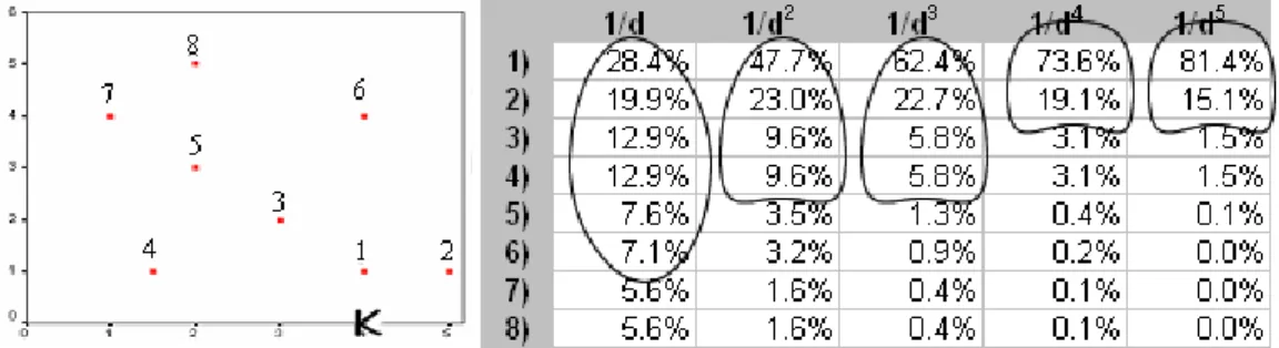
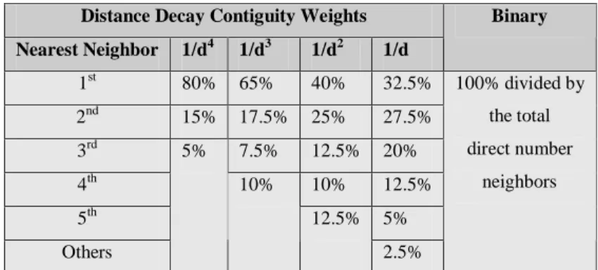
Table 4 – The standard global G and I indices.________________________________________ 68 Table 5 – The SAR benchmark by Li [1996]._________________________________________ 71 Table 6 – The average weights for the first four distance decay contiguities and the binary one. _ 86 Table 7 – The Moran I results according to distance decay contiguities. ____________________ 87 Table 8– The number of direct neighbors according to the binary contiguity of some San Diego districts. ______________________________________________________________________ 89 Table 9– The two geographical arrangements for two datasets. ___________________________ 99 Table 10– Univariate statistics. ___________________________________________________ 105 Table 11– Bivariate statistics. ____________________________________________________ 105 Table 12– Univariate spatial descriptors. ___________________________________________ 106 Table 13 – A global behavior comparison of previous variogram models [Geostatistics FAQ, 1997]. ____________________________________________________________________________ 121 Table 14 – The major differences between Kriging and other interpolation methods._________ 135 Table 15 – Spatial data characteristics by Openshaw [1994].____________________________ 139 Table 16– Internet economic indicators: The evidence. ________________________________ 149 Table 17 – Analysis of geostatistical software._______________________________________ 171 Table 18– The Kriging strategies for the same Nebraska (USA) dataset. __________________ 178 Table 19 – Moran I according to various covariograms ranges for the Africa GDP dataset. ____ 217 Table 20 – The Moran variance scatterplot results for the five cases above. ________________ 230 Table 21 – The SAKWeb® OK estimations for the Pb dataset. __________________________ 254 Table 22 – The SAKWeb® OK estimations for the San Diego housing costs. _______________ 255 Table 23 – The ASP® (server-side) code that produces the VBScript® (client-side) one. ______ 262 Table 24 – Mortality among grasshoppers exposed to insecticide in laboratory and field trials [Onsager, 1978]. ______________________________________________________________ 292 Table 25 – Costs and returns associated with control of grasshoppers (forage was valued at $44 per metric ton and grasshopper density was 10 to 15 per m2) [Onsager, 1978]._________________ 293 Table 26 – SAKWeb© aspatial descriptive results for the four grasshopper datasets. _________ 297 Table 27 – Aspatial descriptive results according to each year and region. _________________ 298 Table 28 – SAKWeb© nearest neighborhood analysis of the four grasshoppers datasets. ______ 300
Table 29 – SAKWeb© Moran’s I correlogram for the grasshopper dataset. _________________ 301 Table 30 – SAKWeb© variogram models for the four datasets. __________________________ 304 Table 31 – The SAKWeb© overall variogram for the years of 1993, 1994, 1995 and 1997. ____ 306 Table 32 – Main trends in the Moran I correlogram and the variogram parameters. __________ 312 Table 33 – Comparison of EGV, classical variance and variogram sill results for the four years. 316 Table 34 – SAKWeb© OK and OK variance with measurement error (30%) of grasshopper Colorado (1993). ______________________________________________________________ 317 Table 35 – SAKWeb© OK and OK variance with measurement error (20% with a rescaled variogram sill factor of 0.7602) for the grasshopper dataset, Colorado (1994). ______________ 318 Table 36 – SAKWeb© OK and OK variance with measurement error (20%) for the grasshopper, Colorado (1995). ______________________________________________________________ 319 Table 37 – SAKWeb© OK and OK variance with measurement error (20%) for the grasshopper, Colorado (1997). ______________________________________________________________ 320 Table 38 – According to the two variogram ranges, the error comparison for the 1993 and 1994 grasshopper datasets clearly demonstrates the appropriate hints of the Moran I correlogram. __ 322 Table 39 – The grasshopper cross-validation for 1993, 1994 (upper row), 1995 and 1997 (lower row). _______________________________________________________________________ 323 Table 40 – The global confidence interval for a level of 80% and a cutoff value of 9 with an OK model without C0. _____________________________________________________________ 325 Table 41 – The local confidence interval for a level of 80% and a cutoff value of 9 with an OK model without C0. _____________________________________________________________ 326 Table 42 – The grasshopper analysis of cross-validation for 1993, 1994, 1995 and 1997 (OK model with C0). ____________________________________________________________________ 328
LIST OF EQUATIONS
Equation 1 – The Chi-Square of statistical interdependency among regions and groups. 57
Equation 2 – The Cressie [1993] resistant variogram estimator. 63
Equation 3 – The spatial lag pies. 64
Equation 4 – The Moran I. 65
Equation 5 – The Geary C. 66
Equation 6 – The local Gi(d). 68
Equation 7 – The global G(d). 68
Equation 8 – The local Moran. 69
Equation 9 – The SAR model. 70
Equation 10 – The variance of SAR model. 70
Equation 11 – The alternative SAR model. 71
Equation 12 – The alternative SAR variance model. 71
Equation 13 – The Columbus, Ohio, OLS model by Anselin [1992]. 72
Equation 14 – The MLE spatial lag model of Columbus, Ohio [Anselin, 1992]. 72
Equation 15 – The error assessment of the multiple regression model. 73
Equation 16 – The OLS regression model of the Brown [1996] Rwanda case. 74
Equation 17 – The MLE spatial lag model of the Brown [1996] Rwanda case. 75
Equation 18 – The regression model of the US government expenditure. 75
Equation 19 – The new regression model of the US government expenditure. 76
Equation 20 – The standard negative residuals contiguity of the binary approach. 76
Equation 21 – The standard positive residuals contiguity of the binary approach. 76
Equation 22 – The standard negative-positive residuals contiguity of binary approach. 77
Equation 23 – The linear estimator. 78
Equation 24 – The distance decay model by Upton [1992]. 80
Equation 25 – The clockwise rotation angle of the standard deviational ellipse. 85
Equations 26 and 27 – The shorter and the longer axes lengths of the standard deviational ellipse. 85
Equation 28 – The pyritic sulfur prediction formula. 97
Equations 29 and 30 – The stationary assumptions. 99
Equations 31 and 32 – The intrinsic hypothesis. 100
Equation 33 – The variogram definition. 100
Equation 34 – The variogram definition for intrinsic variables. 100
Equation 35 – The variogram estimator. 101
Equation 36 – The interpolation structure component. 103
Equation 37 – The Chi-square Normal distribution test. 107
Equation 38 – The Sichel optimal estimator for the lognormal arithmetic mean. 108
Equation 39 – The exponential OLS linear for the regression back (bias) transformation. 108 Equation 40 – The exponential OLS linear regression for the back (unbiased)
transformation. 108
Equation 41 – The back (unbiased) transformation of LK. 108
Equation 42 –The G goodness of prediction index. 109
Equation 43 – The lognormal linear correlation coefficient between elevation and zinc. 110
Equation 44 – The relative variogram. 115
Equation 45 – The general relative variogram. 116
Equation 46 – The pairwise relative variogram. 116
Equation 47 – The geometric anisotropic variogram. 117
Equation 48 – The zonal anisotropic variogram. 118
Equation 49 – The spherical variogram. 120
Equation 50 – The exponential variogram. 120
Equation 51 – The Gaussian variogram. 120
Equation 52 – The search radium formula for irregular grid samples. 122
Equation 53 – The Cressie [1993] automatic fitting formula. 123
Equations 54 and 55 – The variogram OK system. 124
Equations 56 and 57 – The covariogram OK system. 124
Equation 58 – The Matheron OK system. 125
Equation 59 – The Universal Soil Loss Equation for the rainfall-rainoff impact. 128
Equation 60 – The estimation of the true population standard deviation. 129
Equation 61 – The population standard deviation confidence interval. 130
Equation 62 – The mean confidence interval. 130
Equation 63 – Estimation of the probability for a specific cutoff value. 130
Equation 64 – The general Kriging variance. 131
Equation 65 – The concise OK variance in terms of the variogram. 131
Equation 66 – The classical local spatial variance. 132
Equation 67 – The exponential variogram for the San Diego dataset. 213
Equations 68 and 69 – The neighborhood linear regressions for the San Diego dataset. 214 Equation 70 – The spherical variogram for the Africa population density dataset. 216
Equation 71 – The spherical variogram for the Africa GDP dataset. 216
Equations 72 and 73 – The SAKWeb© Moran variance scatterplot. 229
Equation 74 – The Geostatistical Analyst® factor to add concerning the outer rectangle
boundary. 236
Equation 75 – The estimated global mean formula. 238
Equation 76 – The estimated global variance formula. 238
Equation 77 - The exponential variogram for the San Diego dataset. 238
Equation 78 – The new exponential variogram for the San Diego dataset. 238 Equation 79 – The new spherical variogram for the Africa GDP dataset. 239 Equation 80 – The new spherical variogram for the Africa population density dataset. 239
Equation 81 – The non-convexity property. 243
Equation 83 – The combined OK estimates for three datasets. 270
1. Introduction
1.1. STATEMENT OF THE PROBLEM
The problem of statistical spatial analysis encompasses an expanding range of methods which address different spatial problems, from image enhancement and pattern recognition to spatial interpolation and socio-economic trend modeling. Each of these methods focuses on a particular aspect but what emerges is something that is clearly identifiable as spatial statistics, geographically raw data correlated by statistical methods.
Bação [1997], Anselin [1998] and Longley et al. [2001] argue that within specialized software there is a lack of spatial analysis techniques in general and of spatial statistics in particular. This may be a major impediment to GIS, which is a ‘data rich, theory poor’ environment. These authors put an emphasis on creativity, comparing spatial analysis to art and not to science. Applied geostatistics is a talent science because its results may be widely diverse depending on several factors such as the variogram modeling, the Kriging approach, the sampling design or the scientist’s previous experience.
“Very few existing GIS packages have truly analytical functionality” [Levine, 1997, Wong and Lee, 2001]. There has been little progress in incorporating advanced spatial techniques into commercial GIS products in comparison to simple analytical functions. “Most of the functionalities should be more properly regarded as data manipulation rather than analysis” [Openshaw, 1998]. These functions are quite deterministic and include routing, site location, data summarization or vector-raster conversion. Future GIS issues should be viewed as questions of probabilistic thinking, e.g. the Modifiable Areal Unit Problem and Monte Carlo error propagation during an overlay operation.
“At present, most of the literature on statistics for geography should be seen for what it really is: a series of introductions to statistical methods that are of geographical interest only because they have been applied to spatial datasets” [Openshaw 1994, Christensen, 1999]. Such applications are aspatial since they ignore the special characteristics of spatial data such as spatial dependence (autocorrelation) and spatial heterogeneity (association). Hence, it is analysis of spatial data, not spatial analysis of data. It is essential to implement spatial analysis tools that are simultaneously relevant to GIS users and already available in research.
Every year, dozens of research articles are printed with new spatial analysis methods, involving ever more fields such as stochastic simulation, multivariate geostatistic and spatial correlation. Regrettably, the majority of those ideas end up on the bookshelf without any practical consequence for the spatial analysis user. Algorithms, physical realities and thoughts exist for every person. A theory only succeeds if it leads to a practical purpose. “The spirit of geocomputation is fundamentally about matching the philosophy of science with practice, geometry with application, analysis with local context and technology with environment” [Longley, 1998]. To materialize research findings to the real world is a major dilemma nowadays since some of these methods are relatively crude. They have theoretical and implementation problems that remain to be solved. The validation of such findings by peers is a difficulty as well.
Geographers and major GIS users do not think in spatial terms and do not ask questions about spatial pattern and spatial autocorrelation. The goal of most users is to handle large volumes of spatial data and produce beautiful maps rather than carrying out sophisticated statistical spatial analysis. This leads to a corresponding lack of pressure for such methods to be made available.
Since the space aspect of Tobler’s Law1 is the rule for Mother Nature rather than the exception [Clark and Harper, 2000], the classical and convenient assumption of data independency is in the line of fire and the most common statistical procedures must be rethought. The strength of temporal interaction follows the same principle
too (the time aspect of Tobler’s Law). Activities performed on a succeeding day present a higher autocorrelation than yearly activities. Hence, models that involve statistical dependence are often more realistic.
Because spatial autocorrelation is often present, there is a need for spatial analysis. The inexistence of the assumption of spatial independence would create a chaotic basis for natural phenomena. “Hell might be a world without spatial dependence since it would be impossible to live there in any practical and meaningful way” [Longley et al., 2001]. However, random spatial autocorrelation is difficult to detect visually because patches display similar information while others contain fragmented locational information. Most real world patterns are somewhere between a random and a clustered pattern. “Very rarely would we find a spatial pattern that is extremely clustered, extremely dispersed or purely random” [Wong and Lee, 2001].
Some measures of spatial autocorrelation such as the Moran I index try to summarize a complete spatial distribution in a single number. This can lead to a serious flaw: with large spatial datasets, this global measure of spatial autocorrelation can hide spatial heterogeneity or local patterns of spatial clustering.
Spatial residual autocorrelation measurement is crucial although it might not be easy to carry out because most available techniques rely on topological concepts and topology normally stored in a GIS. The common approach consists of using an intermediate application to transfer topological information from the GIS to the statistics application. Naturally, in this situation it is necessary to switch back and forth between the GIS and the analytical tool. On the other hand, “it has been accepted that in the presence of a great number of data points the computation is very intensive and it is probably better handled with specialized software than by integration into the GIS” [Cassetari, 1993].
Neighborhood definition can be difficult for the computation of spatial autocorrelation indices. Mayhew [1999] presents two divergent views: “…where inhabitants recognize each other by sight” versus “others deny the existence of
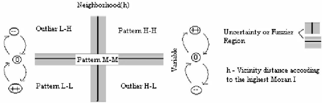
identifiable subculture areas…neighborhoods do not really exist”. Moran I, Geary C, Lisa, the spatial lag pies and the Moran scatterplot embrace consequences of this constraint. In the same way, spatial autocorrelation and association indices reduce vicinity to a single mean (first moment) but this they do not consider the variance (second moment) regarding the neighborhood distribution. Time, cost and convenience represent different aspects to be considered as well.
Concerning software implementation of spatial statistics, several approaches have been made, e.g., specialized software, commercial GIS modules or direct linkage between GIS and statistical packages. From the programmer’s perspective, the most important potential benefit between the latter two approaches involves direct access to spatial query and spatial objects while, at the same time, deriving spatial properties and relationships such as area, distance, adjacency or distance along a network. When spatial objects are areas, spatial properties are essential to compute spatial indices (namely the W weight matrix). However, Figure 1 reveals three problematic situations: the area A centroid is a non-neighbor of area C although its distance is closer than d while area E has no neighbors. The U-shaped region R has its centroid on polygon S. Finally, the four corners of the United States raise neighborhood questions such as whether Utah is a natural neighbor of New Mexico. If spatial objects are points, then defining their neighborhood is even more problematic because of the total lack of natural boundaries.
Figure 1 – The problems in specifying parameters for area objects.
Interpolation quality is a result of the number and distribution of the known points used and how well the mathematical function correctly models the phenomena. Thus, the choice of the appropriate model is essential if reasonable results are to be obtained. For example, with a low inverse distance exponent or high radius, each
local mean moves toward the overall sample mean, leading to a smoother density surface. In contrast, the density surface becomes relatively rough.
Major physical functions and chemical laws are deterministic and based on mathematical expressions. On the contrary, spatial interpolation, an intelligent guesswork process, must include error, autocorrelation, anisotropy and uncertainty constraints where observations are the result of a random process with spatial dependence.
Coined by Matheron at the Institute for Mathematical Morphology in Fontainebleau, Kriging takes into account the trend of each vicinity point for prediction but emphasizes the apparently contradictory aspects of regionalized variables: a random local process versus a structured large-scale one. “For this author, randomness is a fluctuation, not an error of the phenomena with its own structure” [Armstrong, 1998]. Once the structural analysis is made, the estimation can be achieved more accurately using the rate at which the variance between points changes over space. This distinctive feature is expressed by the variogram. However, it assumes that a surface holds a constant mean, a situation almost never true [Nalder and Wein, 1998]. Spatial autocorrelation exists and samples follow a Gaussian distribution. The more severely these assumptions are violated, the less accurate interpolation results become.
The variogram estimation includes a set of parameters2 to be setup by the expert user for implementation. According to Kelly [1996], “there is little to be gained by making Kriging and spatial autocorrelation a main tool of spatial analysis unless the GIS user sophistication is sufficient for this information to be preferred”. Major Kriging software offers a wide range of options but its interpretation requires a thorough background. Certainly, an essential foundation of GIScience is the availability of spatially-aware professionals. Finding the best variogram fitness procedure (interactive or automatic) can also be a problem.
Because estimation error cannot be avoided, Ordinary Kriging variance error is essential for assigning confidence intervals. There is a discrepancy between the
predicted error variance and the real one since in most cases the variogram sill overestimates global sample variance. However, cell declustering and polygonal methods present difficulties in weighting the sample contribution, particularly for the samples on the edge. Outlier negative influence on the variogram and non-sensitivity to data of Ordinary Kriging variance are also real.
Another concern is the assumption of precise and accurate sample values by considering the zero nugget-effect. It is quite common to have a discontinuity at the variogram origin although major Kriging software forces it to be zero at zero distance. On the other hand, if the variogram for zero distance equals total nugget-effect then the estimation Kriging variance becomes lower, leading to a nonsense situation.
1.2. RESEARCH
OBJECTIVES
The research thesis presented here develops the first non-commercial application service provider dealing with spatial autocorrelation measurement, Ordinary Kriging with the Internet Explorer® interface and hypermedia help in an e-Learning context.
The research objectives proposed are:
• To discuss spatial statistical analysis implementation in software and classical statistical limitation with regard to spatial data.
• To investigate and compare IDW and binary approaches regarding W matrix construction on Moran I and the Moran scatterplot.
• To be aware of variography and theoretical Kriging concepts.
• To analyze nugget-effect, range, model and sill rescaling factors in Kriging in conjunction with spatial autocorrelation measures.
• To evaluate Kriging software features at present and to explore Web programming technologies available nowadays.
• To create the first spatial autocorrelation and Ordinary Kriging Web software with the following major characteristics:
• To build a Web interface where simplicity is fundamental.
• To offer a hypermedia help facility in an e-Learning framework.
• To investigate spatial distribution measures like the standard distance deviation and the nearest neighbor index.
• To include brushing with updated local statistical results and indicator maps (based on the conventional and nearest weighted cumulative histogram) for the original samples.
• To compute the first trend surface analysis3 with the join count statistics of its residuals. This includes the location discrimination of positive and negative residuals.
• To plot the Moran I correlogram.
• In accordance with the highest Moran I and variogram contiguity4 function, to create the conventional and Moran location scatterplot in a dynamic mapping structure and dataset renewal. The Moran scatterplot correlogram may also lead to a re-estimated process of the variogram parameters. The IDW deterministic interpolation is also based on the same parameters.
• To plot the Moran variance scatterplot on the basis of the mean variance among neighbors and between the center location and its neighbors.
• To monitor interactive variogram fitness including the azimuth angle factor, anisotropy map, major and minor range, main direction, correlogram, madogram, general relative variogram, pairwise relative variogram, spatial structure proportion and variogram fitness indicator.
• To handle the nugget-effect of four available strategies including differences in results.
• To combine the Kriged estimates by their estimation variances on the basis of the three exact OK models.
• To rescale the variogram function for a higher Ordinary Kriging variance and global and local assessment of area confidence interval.
• To map validation with an extra dataset and cross-validation. This includes the location of true-false positive and negative samples based on the latter analysis.
• To layout an image file with the site mapping in an additional window.
• To delineate interactively the profile of any OK 3D surface to 2D.
• To launch a new menu for other forms of Kriging such as SK, UK, IK and CK.
• To analyze the Colorado, USA, grasshopper case with SAKWeb©.
1.3. CONSTRAINTS AND LIMITATIONS
The present research will be based on the next constraints and limitations:
• Samples hold the same support (the affine and the indirect lognormal correction are not taken into account).
• Observation values are not negative.
• Only one variable at a time is estimated.
• GLS, WLS, Bayesian and stepwise regression, logbit models and the minimum Chi-square method for the Bernoulli and Poisson probability functions, time-series residual correlation, non-parametric tests for data sample comparison such as the Durbin-Watson test, Kruskal-Wallis H, Chi-Square and U Mann-Whitney, non-stationary regionalized variables and Bayesian interpolation, Grubb’s outlier test and geostatistical simulation models are not included in the scope of the research.
• Any type of artificial intelligence (expert systems, genetic algorithms, fuzzy logic, neural networks and hybrid systems) and temporal space analysis are not covered.
1.4. HYPOTHESIS
The research will be based on the following premises:
• There is a lack of knowledge regarding spatial autocorrelation and Kriging issues among Portuguese GIS users.
• Spatial autocorrelation and Kriging software within W3 with hypermedia help in an e-Learning context contributes to the educational sharing and effortless accessing of spatial analysis tools among common users.
• IDW is not a good process for the W specification because it is not sensitive to its natural neighbours such as binary or standard deviational ellipse.
• It is possible to create an uncertainty measure that is both data and geometry dependent.
• A spatial neighborhood pattern can be found regarding which nugget-effect approach fits best. It is expected that in stable and transition regions, a low and a high C0, respectively, will fit best.
• By implementing the variogram sill rescaling based on nearest neighborhood analysis enhances the region confidence interval centered on the Ordinary Kriging variance.
• The Variogram - Moran I - Moran scatterplot optimal SAKWeb© approach helps users as an ESDA tool. In addition, it can help the estimation of variogram parameters in a continuous process.
• The Moran variance scatterplot uncovers observations whose variability is quite different. It can also be used with residuals to locate heteroskedasticity in a detrend Kriging process and particularly significant to validate the stationary assumptions.
1.5. METHODOLOGY
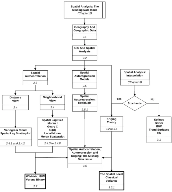
The methodology used is presented in Figures 2, 3, 4, 5, 6 and 7. They give an overview of the methodology, including five major topics:
1) Spatial analysis: The missing data issue; 2) Spatial analysis: Interpolation;
3) Spatial analysis: Implementation review and software evaluation; 4) Spatial analysis: User know-how;
5) SAKWeb© structure and functionalities, including an evaluation survey, enhancements and a spatial data analysis of the Colorado (USA) grasshopper dataset. Spatial Analysis: Users Know-how Chapter 6 SAKWeb (Fig. 5) Chapter 7 Spatial Analysis of Grasshopper Dataset of Colorado, USA Chapter 8 Spatial Analysis: The
Missing Data Issue (Fig. 3) Chapter 2 Spatial Analysis: Interpolation (Fig. 3) Chapter 3 Spatial Analysis: Implementation Review And Software Evaluation
(Fig. 4) Chapter 4 and 5
Theme
Where the topic is developed
Theme (Expanded in
figure X)
1.5.1.
Spatial Analysis: The Missing Data Issue
According to Rogerson, Fotheringham [1996] and Walter [2001], “there is an increased demand for systems that do more than display and organize data”. The set of potential applications for spatial analysis is enormous, for example, accident patterns, victim profiles within a residential population and spread rates for pollution levels. “Techniques are needed to let spatial data speak for themselves” [Griffith and Layne, 1999]. Thus, spatial statistics must hold a specific spatial framework to apply quantitative and statistical methods for a better understanding of spatial relationships. If the finding of spatial structures is fundamental then autocorrelation, interpolation and autoregressive models5 are three major spatial methods that fulfill this constraint. These methods are reviewed here. Although these fields have been developed autonomously, Figure 3 gives the details of the missing data issue that involves the estimation of missing georeferenced data when undertaking spatial autoregression and Kriging. However, spatial autocorrelation can also be exploited for spatial prediction purposes such as patterns and outliers. Spatial autocorrelation measures can also indicate if there is an equally likely chance of predicting neighboring values while the degree of redundancy indicates how much information is free to vary. As expected, certain issues emerged during the review of existing literature, such as:
• The dependence of the OK uncertainty measure solely on geometry;
• Definition of the relationships that exist among the above three concepts;
• W matrix codification;
• Heavy spatial analysis computation;
• Standardization of observation distribution and the impact of sampling approaches.

![Figure 11 – Residual plots where the x-axis represents the predicted values while the y-axis is the associated error [Clark and Hosking, 1986]](https://thumb-eu.123doks.com/thumbv2/123dok_br/15724189.1070813/74.892.257.660.109.347/figure-residual-represents-predicted-values-associated-clark-hosking.webp)