Accepted Manuscript
Improving Imbalanced Learning Through a Heuristic Oversampling
Method Based on K-Means and SMOTE
Georgios Douzas, Fernando Bacao, Felix Last
PII:
S0020-0255(18)30499-7
DOI:
10.1016/j.ins.2018.06.056
Reference:
INS 13749
To appear in:
Information Sciences
Received date:
15 January 2018
Revised date:
11 May 2018
Accepted date:
21 June 2018
Please cite this article as: Georgios Douzas, Fernando Bacao, Felix Last, Improving Imbalanced
Learn-ing Through a Heuristic OversamplLearn-ing Method Based on K-Means and SMOTE, Information Sciences
(2018), doi:
10.1016/j.ins.2018.06.056
This is a PDF file of an unedited manuscript that has been accepted for publication. As a service
to our customers we are providing this early version of the manuscript. The manuscript will undergo
copyediting, typesetting, and review of the resulting proof before it is published in its final form. Please
note that during the production process errors may be discovered which could affect the content, and
all legal disclaimers that apply to the journal pertain.
ACCEPTED MANUSCRIPT
Improving Imbalanced Learning
Through a Heuristic Oversampling Method
Based on K-Means and SMOTE
Georgios Douzasa, Fernando Bacaoa,∗, Felix LastaaNova Information Management School, Campus de Campolide, 1070-312 Lisboa, Portugal Telephone: +351 21 382 8610
Abstract
Learning from class-imbalanced data continues to be a common and challenging problem in supervised learning as standard classification algorithms are designed to handle balanced class distributions. While different strategies exist to tackle this problem, methods which generate artificial data to achieve a balanced class distribution are more versatile than modifications to the classification algorithm. Such techniques, called oversamplers, modify the training data, allowing any classifier to be used with class-imbalanced datasets. Many algorithms have been proposed for this task, but most are complex and tend to generate unnecessary noise. This work presents a simple and effective oversampling method based on k-means clustering and SMOTE (synthetic minority oversampling technique), which avoids the generation of noise and effectively overcomes imbalances between and within classes. Empirical results of extensive experiments with 90 datasets show that training data oversampled with the proposed method improves classification results. Moreover, k-means SMOTE consistently outperforms other popular oversampling methods. An implementation1 is
made available in the Python programming language.
Keywords: Class-Imbalanced Learning, Oversampling, Classification, Clustering, Supervised Learning, Within-Class Imbalance
1. Introduction
The class imbalance problem in machine learning describes classification tasks in which classes of data are not equally represented. In many real-world applications, the nature of the problem implies a sometimes heavy skew in the class distribution of a binary or multi-class classification problem. Such applications include fraud detection in banking, rare medical diagnoses, and oil spill recognition in satellite images, all of which naturally exhibit a minority class [4, 18, 28, 29].
The predictive capability of classification algorithms is impaired by class imbalance. Many such algorithms aim at maximizing classification accuracy, a measure which is biased towards the majority class. A classifier can achieve high classification accuracy even when it does not predict a single minority class instance correctly. For example, a trivial classifier which scores all credit card transactions as legit will score a classification accuracy of 99.9% assuming that 0.1% of transactions are fraudulent; however in this case, all fraud cases remain undetected. In conclusion, by optimizing classification accuracy, most algorithms assume a balanced class distribution [29, 40].
∗Corresponding author
Email addresses: [email protected] (Georgios Douzas), [email protected] (Fernando Bacao), [email protected] (Felix Last)
ACCEPTED MANUSCRIPT
Another inherent assumption of many classification algorithms is the uniformity of misclassification costs, which is rarely a characteristic of real-world problems. Typically in imbalanced datasets, misclassifying the minority class as the majority class has a higher cost associated with it than vice versa. An example of this is database marketing, where the cost of mailing to a non-respondent is much lower than the lost profit of not mailing to a respondent [10].
Lastly, what is referred to as the “small disjuncts problem” is often encountered in imbalanced datasets [18]. The problem refers to classification rules covering only a small number of training examples. The presence of only few samples make rule induction more susceptible to error [25]. To illustrate the importance of discover-ing high quality rules for sparse areas of the input space, the example of credit card fraud detection is again considered. Assume that most fraudulent transactions are processed outside the card owner’s home country. The remaining cases of fraud happen within the country, but show some different exceptional characteristic, such as a high amount, an unusual time or recurring charges. Each of these other characteristics applies to only a very small group of transactions, which by itself is often vanishingly small. However, adding up all these edge cases, they can make up a substantial portion of all fraudulent transactions. Therefore, it is important that classifiers pay adequate attention to small disjuncts [25].
Techniques aimed at improving classification in the presence of class imbalance can be divided into three broad categories2: algorithm level methods, data level methods, and cost-sensitive methods.
Solutions which modify the classification algorithm to cope with the imbalance are algorithm level tech-niques [18, 28]. Such techtech-niques include changing the decision threshold and training separate classifiers for each class [6, 28].
In contrast, cost-sensitive methods aim at providing classification algorithms with different misclassification costs for each class. This requires knowledge of misclassification costs, which are dataset-dependent and commonly unknown or difficult to quantify. Additionally, the algorithms must be capable of incorporating the misclassification cost of each class or instance into their optimization. Therefore, these methods are regarded as operating both on data and algorithm level [18].
Finally, data-level methods manipulate the training data, aiming to change the class distribution towards a more balanced one. Techniques in this category resample the data by removing cases of the majority classes (undersampling) or adding instances to the minority classes by means of duplication or generation of new samples (oversampling) [18, 28]. Because undersampling removes data, such methods risk the loss of impor-tant concepts. Moreover, when the number of minority observations is small, undersampling to a balanced distribution yields an undersized dataset, which may in turn limit classifier performance. Oversampling, on the other hand, may encourage overfitting when observations are merely duplicated [47]. This problem can be avoided by adding genuinely new samples. One straightforward approach to this is synthetic minority over-sampling technique (SMOTE), which interpolates existing samples to generate new instances.
Data-level methods can be further discriminated into random and informed methods. Unlike random meth-ods, which randomly choose samples to be removed or duplicated, informed methods take into account the distribution of the samples [6]. This allows informed methods to direct their efforts to critical areas of the input space, for instance to sparse areas [37], safe areas [3], or to areas close to the decision bound-ary [21]. Consequently, informed methods may avoid the generation of noise and can tackle imbalances within classes.
Unlike algorithm-level methods, which are bound to a specific classifier, and cost-sensitive methods, which are problem-specific and need to be implemented by the classifier, data-level methods can be universally applied and are therefore more versatile [18].
Many oversampling techniques have proven to be effective in real-world domains. SMOTE is the most popular oversampling method that was proposed to improve random oversampling. There are multiple variations of SMOTE which aim to combat the original algorithm’s weaknesses. Yet, many of these approaches are
2The three categories are not exhaustive and new categories have been introduced, such as the combination of each of these techniques with ensemble learning [12, 18, 19].
ACCEPTED MANUSCRIPT
either very complex or alleviate only a few of SMOTE’s shortcomings. Additionally, few of them are readily available in a unified software framework used by practitioners.
This paper suggests the combination of the k-means clustering algorithm with SMOTE to combat some of other oversampler’s shortcomings with a simple-to-use technique. The use of clustering enables the proposed oversampler to identify and target areas of the input space where the generation of artificial data is most effective. The method aims at eliminating both between-class imbalances and within-class imbalances while at the same time avoiding the generation of noisy samples. Its appeal is the widespread availability of both underlying algorithms as well the effectiveness of the method itself.
While the proposed method could be extended to cope with multi-class problems, the focus of this work is placed on binary classification tasks. When working with more than two imbalanced classes, different aspects of classification, as well as evaluation, must be considered, which is discussed in detail by Fern´andez et al. [14].
The remainder of this work is organized as follows. In section 2, related work is summarized and currently available oversampling methods are introduced. Special attention is paid to oversamplers which - like the proposed method - employ a clustering procedure. Section 3 explains in detail how the proposed oversampling technique works and which hyperparameters need to be tuned. It is shown that both SMOTE and random oversampling are limit cases of the algorithm and how they can be achieved. In section 4, a framework aimed at evaluating the performance of the proposed method in comparison with other oversampling techniques is established. The experimental results are shown in section 5, which is followed by section 6 presenting the conclusions.
2. Related Work
Methods to cope with class imbalance either alter the classification algorithm itself, incorporate misclas-sification costs of the different classes into the clasmisclas-sification process, or modify the data used to train the classifier. Resampling the training data can be done by removing majority class samples (undersampling) or by inflating the minority class (oversampling). Oversampling techniques either duplicate existing obser-vations or generate artificial data. Such methods may work uninformed, randomly choosing samples which are replicated or used as a basis for data generation, or informed, directing their efforts to areas where oversampling is deemed most effective. Among informed oversamplers, clustering procedures are sometimes applied to determine suitable areas for the generation of synthetic samples.
Random oversampling randomly duplicates minority class instances until the desired class distribution is reached. Due to its simplicity and ease of implementation, it is likely to be the method that is most frequently used among practitioners. However, since samples are merely replicated, classifiers trained on randomly oversampled data are likely to suffer from overfitting3[2, 6].
In 2002, Chawla et al. [4] suggested the SMOTE algorithm, which avoids the risk of overfitting faced by random oversampling. Instead of merely replicating existing observations, the technique generates artificial samples. As shown in figure 1, this is achieved by linearly interpolating a randomly selected minority observation and one of its neighboring minority observations. More precisely, SMOTE executes three steps to generate a synthetic sample. Firstly, it chooses a random minority observation ~a. Among its k nearest minority class neighbors, instance ~b is selected. Finally, a new sample ~x is created by randomly interpolating the two samples: ~x = ~a + w× (~b − ~a), where w is a random weight in [0, 1].
However, the algorithm has some weaknesses dealing with imbalance and noise as illustrated in figure 2. One such drawback stems from the fact that SMOTE randomly chooses a minority instance to oversample with uniform probability. While this allows the method to effectively combat between-class imbalance, the issues
3Overfitting occurs when a model does not conform with the principle of parsimony. A flexible model with more parameters than required is predisposed to fit individual observations rather than the overall distribution, typically impairing the model’s ability to predict unseen data [22]. In random oversampling, overfitting may occur when classifiers construct rules which seemingly cover multiple observations, while in fact they only cover many replicas of the same observation [2].
ACCEPTED MANUSCRIPT
Figure 1: SMOTE linearly interpolates a randomly selected minority sample and one of its k = 4 nearest neighbors
of within-class imbalance and small disjuncts are ignored. Input areas counting many minority samples have a high probability of being inflated further, while sparsely populated minority areas are likely to remain sparse [39].
Another major concern is that SMOTE may further amplify noise present in the data. This is likely to happen when linearly interpolating a noisy minority sample, which is located among majority class instances, and its nearest minority neighbor. The method is susceptible to noise generation because it doesn’t distinguish overlapping class regions from so-called safe areas [3, 41, 45, 49].
Figure 2: SMOTE may generate minority samples in majority regions in the presence of noise. Most non-noise samples are generated in already dense minority areas, contributing to within-class imbalance.
Despite its weaknesses, SMOTE has been widely adopted by researchers and practitioners, likely due to its simplicity and added value with respect to random oversampling. Numerous modifications and extensions of the technique have been proposed, which aim to eliminate its disadvantages. Such modifications typically address one of the original method’s weaknesses [46]. They may be divided according to their claimed goal into algorithms which aim to emphasize certain minority class regions, intend to combat within-class imbalance, or attempt to avoid the generation of noise.
Focusing its attention on the decision boundary, borderline-SMOTE1 belongs to the category of methods emphasizing class regions. It is the only algorithm discussed here which does not employ a clustering procedure and is included due to its popularity. The technique replaces SMOTE’s random selection of
ACCEPTED MANUSCRIPT
observations with a targeted selection of instances close to the class border. The label of a sample’s k nearest neighbors is used to determine whether it is discarded as noise, selected for its presumed proximity to the class border, or ruled out because it is far from the boundary. Borderline-SMOTE2 extends this method to allow interpolation of a minority instance and one of its majority class neighbors, setting the interpolation weight to less than 0.5 so as to place the generated sample closer to the minority sample [21].
Cluster-SMOTE, another method in the category of techniques emphasizing certain class regions, uses k-means to cluster the minority class before applying SMOTE within the found clusters. The stated goal of this method is to boost class regions by creating samples within naturally occurring clusters of the minority class. It is not specified how many instances are generated in each cluster, nor how the optimal number of clusters can be determined [7]. While the method may alleviate the problem of between-class imbalance, it does not help to eliminate small disjuncts.
Belonging to the same category, adaptive semi-unsupervised weighted oversampling (A-SUWO) introduced by Nekooeimehr and Lai-Yuen [36], is a rather complex technique which applies clustering to improve the quality of oversampling. The approach is based on hierarchical clustering and aims at oversampling hard-to-learn instances close to the decision boundary.
Among techniques which aim to reduce within-class imbalance at the same time as between-class imbalance is cluster-based oversampling. The algorithm clusters the entire input space using k-means. Random over-sampling is then applied within clusters so that: a) all majority clusters, b) all minority clusters, and c) the majority and minority classes are of the same size [27]. By replicating observations instead of generating new ones, this technique may encourage overfitting.
In cluster-based undersampling, Lin et al. [32] apply k-means clustering with k equal to the number of minority samples. Only cluster centroids or cluster medoids are retained for the undersampled majority class, resulting in equally sized classes. Being an undersampling method, this approach removes observations which could represent important concepts.
With a bi-directional sampling approach, Song et al. [44] combine undersampling the majority class with oversampling the minority class. K-means clustering is applied separately within each class with the goal of achieving within- and between-class balance. The undersampling step of this method is identical to cluster-based undersampling [32] retaining cluster medoids with the number of clusters k set to the mean class size. The minority class is clustered into two partitions. Subsequently, SMOTE is applied in the smaller cluster. A number of iterations of clustering and SMOTE are performed until both classes are of equal size. Since this approach clusters both classes separately, it is blind to overlapping class borders and may contribute to noise generation.
The self-organizing map oversampling (SOMO) algorithm transforms the input data into a two-dimensional space using a self-organizing map, where safe and effective areas are identified for data generation. SMOTE is then applied within clusters found in the lower dimensional space, as well as between neighboring clusters in order to correct within- and between-class imbalances [11].
Aiming to avoid noise generation, a clustering-based approach called CURE-SMOTE uses the hierarchical clustering algorithm CURE to clear the data of outliers before applying SMOTE. The rationale behind this method is that because SMOTE would amplify existing noise, the data should be cleared of noisy observations prior to oversampling [33]. While noise generation is avoided, possible imbalances within the minority class are ignored.
Santos et al. [42] cluster the entire input space with k-means. Clusters with few representatives are chosen to be oversampled using SMOTE. The algorithm is different from most oversampling methods in that SMOTE is applied regardless of the class label. The class label of the generated sample is copied from the nearest of the two parents. The algorithm thereby targets dataset imbalance, rather than imbalances between or within classes and cannot be used to solve class imbalance.
An ensemble method designed to improve the prediction of rare classes, called COG, uses k-means to break up the majority class into smaller partitions with the goal of facilitating linear separability. For each cluster of the majority class, a single linear classifier is trained to separate it from the minority class. The final
ACCEPTED MANUSCRIPT
predictor is a conjunction of all inferred rules. The method COG-OS extends this process by applying random oversampling within clusters of the minority class [48]. The distribution of generated samples across minority clusters is left to the user and not guided by any heuristic. Moreover, effective application of COG-OS requires knowledge of the subclustering structure to determine the number of clusters in each class. As such, its application may be unfeasible in large and high-dimensional datasets.
In summary, there has been a lot of recent research aimed at the improvement of imbalanced dataset resampling. Some proposed methods employ clustering techniques before applying random oversampling or SMOTE. While most of them manage to combat some weaknesses of existing oversampling algorithms, none have been shown to avoid noise generation and alleviate imbalances both between and within classes at the same time. Additionally, many techniques achieve their respective improvements at the cost of high complexity, making the techniques difficult to implement and use.
3. Proposed Method
The method proposed in this work employs the simple and popular k-means clustering algorithm in conjunc-tion with SMOTE oversampling in order to rebalance skewed datasets. It manages to avoid the generaconjunc-tion of noise by oversampling only in safe areas. Moreover, its focus is placed on both between-class imbalance and within-class imbalance, combating the small disjuncts problem by inflating sparse minority areas. The method is easily implemented due to its simplicity and the widespread availability of both k-means and SMOTE.
The method is uniquely different from related methods not only due to its simplicity but also because of its novel and effective approach to distributing synthetic samples. Sample distribution is based on cluster density, generating more samples in sparse minority areas than in dense ones in order to combat within-class imbalance. Moreover, the proposed technique is distinguished by the fact that it clusters regardless of class label, enabling the detection of areas safe for oversampling. Finally, overfitting is counteracted by generating new samples instead of replicating them.
3.1. Algorithm
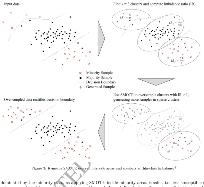
K-means SMOTE consists of three steps: clustering, filtering, and oversampling. In the clustering step, the input space is clustered into k groups using k-means clustering. The filtering step selects clusters for oversampling, retaining those with a high proportion of minority class samples. It then distributes the number of synthetic samples to generate, assigning more samples to clusters where minority samples are sparsely distributed. Finally, in the oversampling step, SMOTE is applied in each selected cluster to achieve the target ratio of minority and majority instances. The algorithm is illustrated in figure 3.
The k-means algorithm is a popular iterative method of finding naturally occurring groups in data which can be represented in a Euclidean space. It works by iteratively repeating two instructions: First, assign each observation to the nearest of k cluster centroids. Second, update the position of the centroids so that they are centered between the observations assigned to them. The algorithm converges when no more observations are reassigned. It is guaranteed to converge to a typically local optimum in a finite number of iterations [34]. For large datasets where k-means may be slow to converge, more efficient implementations could be used for the clustering step of the k-means SMOTE, such as mini-batch k-means as proposed by [43]. All hyperparameters of k-means are also hyperparameters of the proposed algorithm, most notably k, the number of clusters. Finding an appropriate value for k is important for the effectiveness of k-means SMOTE as it influences how many minority clusters, if any, can be found in the filter step.
Following the clustering step, the filter step chooses clusters to be oversampled and determines how many samples are to be generated in each cluster. The motivation of this step is to oversample only clusters
4The rectification of the decision boundary in the lower left of the image is desired because the two majority samples are considered outliers. The classifier is thus able to induce a simpler rule, which is less error prone.
ACCEPTED MANUSCRIPT
Figure 3: K-means SMOTE oversamples safe areas and combats within-class imbalance4
dominated by the minority class, as applying SMOTE inside minority areas is safer, i.e. less susceptible to noise generation. Moreover, the goal is to achieve a balanced distribution of samples within the minority class. Therefore, the filter step allocates more generated samples to sparse minority clusters than to dense ones.
The selection of clusters for oversampling is based on each cluster’s proportion of minority and majority instances. By default, any cluster made up of at least 50 % minority samples is selected for oversampling. This behavior can be tuned by adjusting the imbalance ratio threshold (or irt), a hyperparameter of k-means SMOTE which defaults to 1. The imbalance ratio of a cluster c is defined as majority count(c)+1minority count(c)+1. When the imbalance ratio threshold is increased, cluster choice is more selective and a higher proportion of minority instances is required for a cluster to be selected. On the other hand, lowering the threshold loosens the selection criterion, allowing clusters with a higher majority proportion to be chosen.
To determine the distribution of samples to be generated, filtered clusters are assigned sampling weights between zero and one. A high sampling weight corresponds to a low density of minority samples and yields more generated samples. To achieve this, the sampling weight depends on how dense a single cluster is compared to how dense all selected clusters are on average. Note that when measuring a cluster’s density, only the distances among minority instances are considered. The computation of the sampling weight may be expressed by means of five sub-computations:
ACCEPTED MANUSCRIPT
2. Compute the mean distance within each cluster by summing all non-diagonal elements of the distance matrix, then dividing by the number non-diagonal elements.
3. To obtain a measure of density, divide each cluster’s number of minority instances by its average minor-ity distance raised to the power of the number of features m: densminor-ity(f ) = average minority distance(f )minority count(f ) m.
4. Invert the density measure as to get a measure of sparsity, i.e. sparsity(f ) = 1 density(f ).
5. The sampling weight of each cluster is defined as the cluster’s sparsity factor divided by the sum of all clusters’ sparsity factors.
Consequently, the sum of all sampling weights is one. Due to this property, the sampling weight of a cluster can be multiplied by the overall number of samples to be generated to determine the number of samples to be generated in that cluster.
In the oversampling step of the algorithm, each filtered cluster is oversampled using SMOTE. For each cluster, the oversampling procedure is given all points of the cluster along with the instruction to generate ksampling weight(f) × nk samples, where n is the overall number of samples to be generated. Per synthetic sample to generate, SMOTE chooses a random minority observation ~a within the cluster, finds a random neighboring minority instance ~b of that point and determines a new sample ~x by randomly interpolating ~a and ~b. In geometric terms, the new point ~x is thus placed somewhere along a straight line from ~a to ~b. The process is repeated until the number of samples to be generated is reached.
SMOTE’s hyperparameter k nearest neighbors, or knn, constitutes among how many neighboring minority samples of ~a the point ~b is randomly selected. This hyperparameter is also used by k-means SMOTE. Depending on the specific implementation of SMOTE, the value of knn may have to be adjusted downward when a cluster has fewer than knn + 1 minority samples. Once each filtered cluster has been oversampled, all generated samples are returned and the oversampling process is completed.
The proposed method is distinct from related techniques in that it clusters the entire dataset regardless of the class label. This unsupervised approach enables the discovery of overlapping class regions and may aid the avoidance of oversampling in unsafe areas. This is in contrast to cluster-SMOTE, where only minority class instances are clustered [7] and to the aforementioned combination of oversampling and undersampling where both classes are clustered separately [44]. Another distinguishing feature is the unique approach to the distribution of generated samples across clusters: sparse minority clusters yield more samples than dense ones. The previously presented method cluster-based oversampling, on the other hand, distributes samples based on cluster size [27]. Since k-means may find clusters of varying density, but typically of the same size [34, 48], distributing samples according to cluster density can be assumed to be an effective way to combat within-class imbalance. Lastly, the use of SMOTE circumvents the problem of overfitting, which random oversampling has been shown to encourage.
3.2. Limit Cases
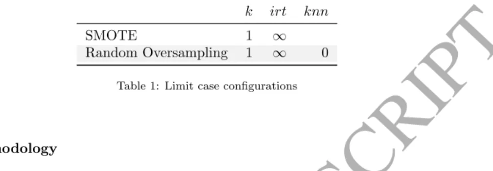
In the following, it is shown that SMOTE and random oversampling can be regarded as limit cases of the more general method proposed in this work. In k-means SMOTE, the input space is clustered using k-means. Subsequently, some clusters are selected and then oversampled using SMOTE. Considering the case where the number of clusters k is equal to 1, all observations are grouped in one cluster. For this only cluster to be selected as a minority cluster, the imbalance ratio threshold needs to be set so that the imbalance ratio of the training data is met. For example, in a dataset with 100 minority observations and 10,000 majority observations, the imbalance ratio threshold must be greater than or equal to 10,000+1100+1 ≈ 99.02. The single cluster is then selected and oversampled using SMOTE; since the cluster contains all observations, this is equivalent to simply oversampling the original dataset with SMOTE. Instead of setting the imbalance ratio threshold to the exact imbalance ratio of the dataset, it can simply be set to positive infinity.
If SMOTE did not interpolate two different points to generate a new sample but performed the random interpolation of one and the same point, the result would be a copy of the original point. This behavior could be achieved by setting the parameter “k nearest neighbors” of SMOTE to zero if the concrete implementation supports this behavior. As such, random oversampling may be regarded as a specific case of SMOTE.
ACCEPTED MANUSCRIPT
Input: X (matrix of observations) y (target vector)
n (number of samples to be generated) k (number of clusters to be found by k-means) irt (imbalance ratio threshold)
knn (number of nearest neighbors considered by SMOTE)
de (exponent used for computation of density; defaults to the number of features in X) begin
// Step 1: Cluster the input space and filter clusters with more minority instances than majority instances.
clusters← kmeans(X) filtered clusters← ∅ for c∈ clusters do
imbalance ratio←minority count(c)+1majority count(c)+1
if imbalance ratio < irt then
filtered clusters← filtered clusters ∪ {c} end
end
// Step 2: For each filtered cluster, compute the sampling weight based on its minority density.
for f ∈ filtered clusters do
average minority distance(f )← mean(euclidean distances(f)) density factor(f )← average minority distance(f )minority count(f ) de
sparsity factor(f )← 1 density factor(f )
end
sparsity sum←Pf∈filtered clusterssparsity factor(f )
sampling weight(f )←sparsity factor(f )sparsity sum
// Step 3: Oversample each filtered cluster using SMOTE. The number of samples to be generated is computed using the sampling weight.
generated samples← ∅ for f ∈ filtered clusters do
number of samples← kn × sampling weight(f)k
generated samples← generated samples ∪ { SMOT E(f, number of samples, knn) } end
return generated samples end
ACCEPTED MANUSCRIPT
This property of k-means SMOTE is of very practical value to its users: since it contains both SMOTE and random oversampling, a search of optimal hyperparameters could include the configurations for those methods. As a result, while a better parametrization may be found, the proposed method will perform at least as well as the better of both oversamplers. In other words, SMOTE and random oversampling are fallbacks contained in k-means SMOTE, which can be resorted to when the proposed method does not produce any gain with other parametrizations. Table 1 summarizes the parameters which may be used to reproduce the behavior of both algorithms.
k irt knn
SMOTE 1 ∞
Random Oversampling 1 ∞ 0
Table 1: Limit case configurations
4. Research Methodology
The ultimate purpose of any resampling method is the improvement of classification results. In other words, a resampling technique is successful if the resampled data it produces improves the prediction quality of a given classifier. Therefore, the effectiveness of an oversampling method can only be assessed indirectly by evaluating a classifier trained on oversampled data. This proxy measure, i.e. the classifier performance, is only meaningful when compared with the performance of the same classification algorithm trained on data which has not been resampled. Multiple oversampling techniques can then be ranked by evaluating a classifier’s performance with respect to each modified training set produced by the resamplers.
A general concern in classifier evaluation is the bias of evaluating predictions for previously seen data. Classifiers may perform well when making predictions for rows of data used during training, but poorly when classifying new data. This problem is also referred to as overfitting. Oversampling techniques have been observed to encourage overfitting, which is why this bias should be carefully avoided during their evaluation. A general approach is to split the available data into two or more subsets of which only one is used during training, and another is used to evaluate the classification. The latter is referred to as the holdout set, unknown data, or test dataset.
Arbitrarily splitting the data into two sets, however, may introduce additional biases. One potential issue that arises is that the resulting training set may not contain certain observations, preventing the algorithm from learning important concepts. Cross-validation combats this issue by randomly splitting the data many times, each time training the classifier from scratch using one portion of the data before measuring its performance on the remaining share of data. After a number of repetitions, the classifier can be evaluated by aggregating the results obtained in each iteration. In k-fold validation, a popular variant of cross-validation, k iterations, called folds, are performed. During each fold, the test set is one of k equally sized groups. Each group of observations is used exactly once as a holdout set. K-fold cross-validation can be repeated many times to avoid potential bias due to random grouping [26].
While k-fold cross validation typically avoids the most important biases in classification tasks, it might distort the class distributions when randomly sampling from a class-imbalanced dataset. In the presence of extreme skews, there may even be iterations where the test set contains no instances of the minority class, in which case classifier evaluation would be ill-defined or potentially strongly biased. A simple and common approach to this problem is to use stratified cross-validation, where instead of sampling completely at random, the original class distribution is preserved in each fold [26].
4.1. Metrics
Of the various assessment metrics traditionally used to evaluate classifier performance, not all are suitable when the class distribution is not uniform. However, there are metrics which have been employed or developed specifically to cope with imbalanced data.
ACCEPTED MANUSCRIPT
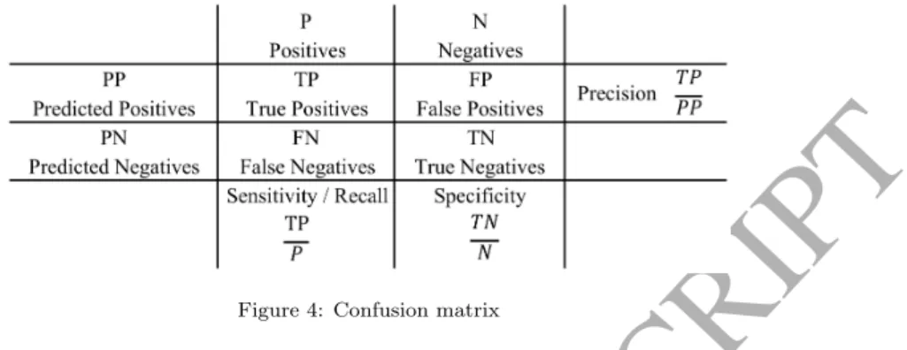
Classification assessment metrics compare the true class membership of each observation with the prediction of the classifier. To illustrate the alignment of predictions with the true distribution, a confusion matrix (figure 4) can be constructed. Possibly deriving from medical diagnoses, a positive observation is a rare case and belongs to the minority class. The majority class is considered negative [26].
Figure 4: Confusion matrix
When evaluating a single classifier in the context of a finite dataset with fixed imbalance ratio, the confusion matrix provides all necessary information to assess the classification quality. However, when comparing dif-ferent classifiers or evaluating a single classifier in variable environments, the absolute values of the confusion matrix are non-trivial.
The most common metrics for classification problems are accuracy and its inverse, error rate. Accuracy = T P + T N
P + N ; Error Rate = 1− Accuracy (1) These metrics show a bias toward the majority class in imbalanced datasets. For example, a naive classifier which predicts all observations as negative would achieve 99% accuracy in a dataset where only 1% of instances are positive. While such high accuracy suggests an effective classifier, the metric obscures the fact that not a single minority instance was predicted correctly [23].
Sensitivity, also referred to as recall or true positive rate, explains the prediction accuracy among minority class instances. It answers the question “How many minority instances were correctly classified as such?” Specificity answers the same question for the majority class. Precision is the rate of correct predictions among all instances predicted to belong to the minority class. It indicates how many of the positive predictions are correct [23].
The F1-score, or F-measure, is the (often weighted) harmonic mean of precision and recall. In other terms, the indicator rates both the completeness and exactness of positive predictions [23, 26].
F 1 =(1 + α)× (sensitivity × precision) sensitivity + α× precision = (1 + α)× (T PP × T P P P) T P P + α× T P P P (2) The geometric mean score, also referred to as g-mean or g-measure, is defined as the geometric mean of sensitivity and specificity. The two components can be regarded as per-class accuracy. The g-measure aggregates both metrics into a single value in [0, 1], assigning equal importance to both [23, 26].
g-mean =psensitivity× specificity = r
T P P ×
T N
N (3)
Precision-recall (PR) diagrams plot the precision of a classifier as a function of its minority accuracy. Clas-sifiers outputting class membership confidences (i.e. continuous values in [0, 1]) can be plotted as multi-ple points in discrete intervals, resulting in a PR curve. Commonly, the area under the precision-recall curve (AUPRC) is computed as a single numeric performance metric [23, 26].
ACCEPTED MANUSCRIPT
The choice of metric depends to a great extent on the goal their user seeks to achieve. In certain practical tasks, one specific aspect of classification may be more important than another (e.g. in medical diagnoses, false negatives are much more critical than false positives). However, to determine a general ranking among oversamplers, no such focus should be placed. Therefore, the following unweighted metrics are chosen for the evaluation.
• g-mean • F1-score • AUPRC 4.2. Oversamplers
The following list enumerates the oversamplers used as a benchmark for the evaluation of the proposed method, along with the set of hyperparameters used for each. The optimal imbalance ratio is not obvious and has been discussed by other researchers [5, 13, 40]. This work aims at creating comparability among over-samplers; consequently, it is most important that oversamplers achieve the same imbalance ratio. Therefore, all oversampling methods were parametrized to generate as many instances as necessary so that minority and majority classes count the same number of samples.
• random oversampling • SMOTE – knn∈ {3, 5, 20} • borderline-SMOTE1 – knn∈ {3, 5, 20} • borderline-SMOTE2 – knn∈ {3, 5, 20} • k-means SMOTE – k∈ {2, 20, 50, 100, 250, 500} – knn∈ {3, 5, 20, ∞} – irt∈ {1, ∞} – de∈ {0, 2, number of features} • no oversampling 4.3. Classifiers
For the evaluation of the various oversampling methods, several different classifiers are chosen to ensure that the results obtained can be generalized and are not constrained to the usage of a specific classifier. The choice of classifiers is further motivated by the number of hyperparameters: classification algorithms with few or no hyperparameters are less likely to bias results due to their specific configuration.
Logistic regression (LR) is a generalized linear model which can be used for binary classification. Fitting the model is an optimization problem which can be solved using simple optimizers which require no hyperpa-rameters to be set [35]. Consequently, results achieved by LR are easily reproducible, while also constituting a baseline for more sophisticated approaches.
Another classification algorithm referred to as k-nearest neighbors (KNN) assigns an observation to the class most of its nearest neighbors belong to. How many neighbors are considered is determined by the method’s hyperparameter k [15].
ACCEPTED MANUSCRIPT
Finally, gradient boosting over decision trees, or simply gradient boosting machine (GBM), is an ensemble technique used for classification. In the case of binary classification, one shallow decision tree is induced at each stage of the algorithm. Each tree is fitted to observations which could not be correctly classified by decision trees of previous stages. Predictions of GBM are made by majority vote of all trees. In this way, the algorithm combines several simple models (referred to as weak learners) to create one effective classifier. The number of decision trees to generate, which in binary classification is equal to the number of stages, is a hyperparameter of the algorithm [16].
As further explained in section 4.5, various combinations of hyperparameters are tested for each classifier. All classifiers are used as implemented in the Python library scikit-learn [38] with default parameters unless stated otherwise. The following list enumerates the classifiers used in this study along with a set of values for their respective hyperparameters.
• LR • KNN – k∈ {3, 5, 8} • GBM – number of trees∈ {50, 100, 200} 4.4. Datasets
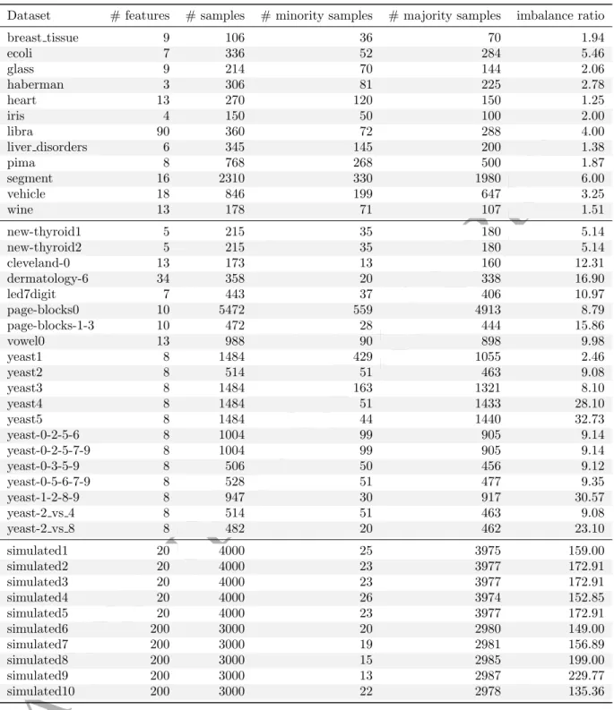
To evaluate k-means SMOTE, 12 imbalanced datasets from the UCI Machine Learning Repository [31] are used. Those datasets containing more than two classes were binarized using a one-versus-rest approach, labeling the smallest class as the minority and merging all other samples into one class. In order to generate additional datasets with even higher imbalance ratios, each of the aforementioned datasets was randomly undersampled to generate up to six additional datasets. The imbalance ratio of each dataset was increased approximately by multiplication factors of 2, 4, 6, 10, 15 and 20, but only if a given factor did not reduce a dataset’s total number of minority samples to less than eight. Furthermore, 19 imbalanced datasets were selected from from the KEEL repository [1]. Lastly, the Python library scikit-learn [38] was used to generate ten variations of the artificial “MADELON” dataset, which poses a difficult binary classification problem [20].
Table 2 lists the datasets used to evaluate the proposed method, along with important characteristics. The ar-tificial datasets are referred to as simulated. Undersampled versions of the original datasets are omitted from the table; in the figures presented in section 5, the factor used for undersampling is appended to the dataset names. All modified and simulated datasets used in the study are made available at https://github.com/ felix-last/evaluate-kmeans-smote/releases/download/v0.0.1/uci_extended.tar.gzfor the purpose of reproducibility.
Additionally, in order to demonstrate the properties of k-means SMOTE, five two-dimensional binary class datasets are introduced. Three of those datasets, which were created for the purpose of this work, consist of observations in three partially noisy clusters. They are referred to as datasets A, B and C and can be found at https://github.com/felix-last/evaluate-kmeans-smote/releases/download/v0.0.2/toy_ datasets.tar.gz. The other two toy datasets were created using the “make circles” and “make moons” functions of scikit-learn with a noise factor of 0.3. 750 samples of each class were generated, before one class was randomly undersampled to 200 observations.
4.5. Experimental Framework
To evaluate the proposed method, the oversamplers, metrics, datasets, and classifiers discussed in this section are used. Results are obtained by repeating 5-fold cross-validation five times. For each dataset, every metric is computed by averaging their values across runs. In addition to the arithmetic mean, the standard deviation is calculated.
ACCEPTED MANUSCRIPT
Dataset # features # samples # minority samples # majority samples imbalance ratio
breast tissue 9 106 36 70 1.94 ecoli 7 336 52 284 5.46 glass 9 214 70 144 2.06 haberman 3 306 81 225 2.78 heart 13 270 120 150 1.25 iris 4 150 50 100 2.00 libra 90 360 72 288 4.00 liver disorders 6 345 145 200 1.38 pima 8 768 268 500 1.87 segment 16 2310 330 1980 6.00 vehicle 18 846 199 647 3.25 wine 13 178 71 107 1.51 new-thyroid1 5 215 35 180 5.14 new-thyroid2 5 215 35 180 5.14 cleveland-0 13 173 13 160 12.31 dermatology-6 34 358 20 338 16.90 led7digit 7 443 37 406 10.97 page-blocks0 10 5472 559 4913 8.79 page-blocks-1-3 10 472 28 444 15.86 vowel0 13 988 90 898 9.98 yeast1 8 1484 429 1055 2.46 yeast2 8 514 51 463 9.08 yeast3 8 1484 163 1321 8.10 yeast4 8 1484 51 1433 28.10 yeast5 8 1484 44 1440 32.73 yeast-0-2-5-6 8 1004 99 905 9.14 yeast-0-2-5-7-9 8 1004 99 905 9.14 yeast-0-3-5-9 8 506 50 456 9.12 yeast-0-5-6-7-9 8 528 51 477 9.35 yeast-1-2-8-9 8 947 30 917 30.57 yeast-2 vs 4 8 514 51 463 9.08 yeast-2 vs 8 8 482 20 462 23.10 simulated1 20 4000 25 3975 159.00 simulated2 20 4000 23 3977 172.91 simulated3 20 4000 23 3977 172.91 simulated4 20 4000 26 3974 152.85 simulated5 20 4000 23 3977 172.91 simulated6 200 3000 20 2980 149.00 simulated7 200 3000 19 2981 156.89 simulated8 200 3000 15 2985 199.00 simulated9 200 3000 13 2987 229.77 simulated10 200 3000 22 2978 135.36
Table 2: Summary of datasets used to evaluate and compare the proposed method (split by data source; top: UCI, middle: KEEL, bottom: generated; some names shortened)
To achieve optimal results for all classifiers and oversamplers, a grid search procedure is used. For this purpose, each classifier and each oversampler specifies a set of possible values for every hyperparameter. Subsequently, all possible combinations of an algorithm’s hyperparameters are generated and the algorithm is executed once for each combination. All metrics are used to score all resulting classifications, and the best value obtained for each metric is saved.
ACCEPTED MANUSCRIPT
To illustrate this process, consider an example with one oversampler and one classifier. The following list shows each algorithm with several combinations for each parameter.
• SMOTE
– knn∈ {3, 6} • GBM
– number of trees∈ {10, 50}
The oversampling method SMOTE is run two times, generating two different sets of training data. For each set of training data, the classifier LR is executed twice. Therefore, the classifier will be executed four times. The possible combinations are:
• knn = 3, number of trees = 10 • knn = 3, number of trees = 50 • knn = 6, number of trees = 10 • knn = 6, number of trees = 50
If two metrics are used for scoring, both metrics score all four runs; the best result is saved. Note that one metric may find that the combination knn = 3, number of trees = 10 is best, while a different combination might be best considering another metric. In this way, each oversampler and classifier combination is given the chance to optimize for each metric.
5. Experimental Results
Following recommendations of Demˇsar [9] for evaluating classifier performance across multiple datasets, obtained scores are not compared directly, but instead ordered to derive a ranking. To adapt the method for the evaluation of oversampling techniques, oversamplers are ranked in place of classication algorithms. Combined with the Friedman test [17] and Holm’s method [24], this evaluation method is also used by other authors working on the topic of imbalanced classification [8, 19, 41].
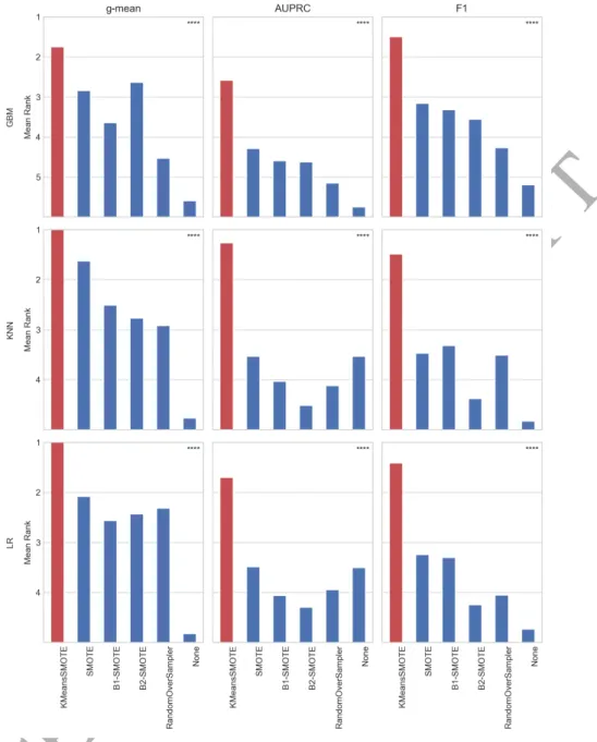
To derive the rank order, cross-validated scores are used, assigning rank one to the best performing and rank six to the worst performing technique. This results in different rankings for each of five experiment repetitions, again partitioned by dataset, metric, and classifier. To aggregate the various rankings, each method’s assigned rank is averaged across datasets and experiment repetitions. Consequently, a method’s mean rank is a real number in the interval [1.0, 6.0]. The mean ranking results for each combination of metric and classifier are shown in figure 5.
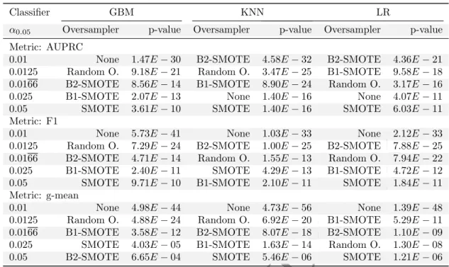
Testing the null hypothesis that differences in terms of rank among oversamplers are merely a matter of chance, the Friedman test determines the statistical significance of the derived mean ranking. The test is chosen because it does not assume normality of the obtained scores. At a significance level of α = 0.05, the null hypothesis is rejected for all evaluated classifiers and evaluation metrics. Therefore, a post-hoc test is applied. Holm’s step-down procedure is applied with the proposed method as the control method. The procedure corrects the significance level downwards to account for multiple testing. The null hypothesis in each pair-wise comparison of the control method and another oversampler is that the control method does not perform better than the other method. Table 3 shows the results of the Holm’s test for all evaluated metrics and classifiers. The null hypothesis is rejected for all oversamplers at a significance level of α = 0.05, indicating that the proposed method outperforms all other methods.
The mean ranking shows that the proposed method outperforms other methods with regard to all evaluation metrics. Notably, the technique’s superiority can be observed independently of the classifier. In eight out of nine cases, k-means SMOTE achieves a mean rank better than two, whilst still better than three in the remaining case. Furthermore, k-means SMOTE is the only technique with a mean ranking better than
ACCEPTED MANUSCRIPT
Figure 5: Mean ranking (best: 1; worst: 6) of evaluated oversamplers for different classifiers and metrics
three with respect to F1 score and AUPRC, boosting classification results when other oversamplers tie or accomplish a similar rank as no oversampling.
Generally, it can be observed that - aside from the proposed method - SMOTE, borderline-SMOTE1, and borderline-SMOTE2 typically achieve the best results, while no oversampling frequently earns the worst rank. Remarkably, LR and KNN achieve a similar rank without oversampling as with SMOTE with regard to AUPRC, while both are only dominated by k-means SMOTE. This indicates that the proposed method may improve classifier performance even in situations where SMOTE is not able to achieve any improvement versus the original training data.
For a direct comparison to the baseline method, SMOTE, the average optimal scores attained by k-means SMOTE for each dataset are subtracted by the respective scores reached by SMOTE. The resulting score
ACCEPTED MANUSCRIPT
Classifier GBM KNN LR
α0.05 Oversampler p-value Oversampler p-value Oversampler p-value
Metric: AUPRC
0.01 None 1.47E− 30 B2-SMOTE 4.58E− 32 B2-SMOTE 4.36E− 21 0.0125 Random O. 9.18E− 21 Random O. 3.47E− 25 B1-SMOTE 9.58E− 18 0.0166 B2-SMOTE 8.56E− 14 B1-SMOTE 8.90E− 24 Random O. 3.17E− 16 0.025 B1-SMOTE 2.07E− 13 None 1.40E− 16 None 4.07E− 11 0.05 SMOTE 3.61E− 10 SMOTE 1.40E− 16 SMOTE 6.03E− 11 Metric: F1
0.01 None 5.73E− 41 None 1.03E− 33 None 2.12E− 33 0.0125 Random O. 7.29E− 24 B2-SMOTE 1.00E− 25 B2-SMOTE 7.88E− 25 0.0166 B2-SMOTE 4.71E− 14 Random O. 1.55E− 13 Random O. 7.94E− 22 0.025 B1-SMOTE 2.40E− 11 SMOTE 4.29E− 13 B1-SMOTE 4.72E− 12 0.05 SMOTE 9.71E− 10 B1-SMOTE 2.10E− 11 SMOTE 1.84E− 11 Metric: g-mean
0.01 None 4.98E− 44 None 4.73E− 56 None 1.39E− 48 0.0125 Random O. 4.88E− 24 Random O. 6.92E− 20 B1-SMOTE 5.29E− 11 0.0166 B1-SMOTE 3.58E− 12 B2-SMOTE 8.07E− 18 B2-SMOTE 1.10E− 09 0.025 SMOTE 4.03E− 05 B1-SMOTE 1.63E− 14 Random O. 1.30E− 08 0.05 B2-SMOTE 6.65E− 04 SMOTE 5.46E− 06 SMOTE 1.21E− 06
Table 3: Results of Holm’s test with k-means SMOTE as the control method
improvements achieved by the proposed method are summarized in figures 6 and 7.
Figure 6: Mean score improvement of the proposed method
versus SMOTE across datasets Figure 7:method versus SMOTEMaximum score improvement of the proposed
The KNN classifier appears to profit most from the application of k-means SMOTE, where maximum score improvements of more than 0.2 are observed across all metrics. The biggest mean score improvements are also achieved using KNN, with average gains ranging from 0.019 to 0.035. It can further be observed that all classifiers benefit from the suggested oversampling procedure. With only one exception, maximum score improvements of more than 0.1 are found for all classifiers and metrics.
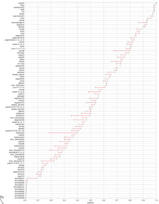
Taking a closer look at one of the combinations of classifier and metric which, on average, benefit most from the application of the proposed method, figure 8 shows the AUPRC achieved per dataset by each of the two oversamplers in conjunction with the KNN classifier. Although absolute scores and score differences between the two methods are dependent on the choice of metric and classifier, the general trend shown in the figure is observed for all other metrics and classifiers, which are omitted for clarity.
ACCEPTED MANUSCRIPT
In the large majority of cases, k-means SMOTE outperforms SMOTE, proving the relevance of the clustering procedure. Only in 6 out of 90 datasets tested there were no improvements through the use of k-means SMOTE. On average, k-means SMOTE achieves an AUPRC improvement of 0.035. The biggest gains of the proposed method appear to be occurring in the score range of 0.2 to 0.8. The biggest gain of approximately 0.2 is achieved for dataset “vehicle20”. The score difference among oversamplers is smaller at the extreme ends of the scale. For nine of the simulated datasets, KNN attains a score very close to zero independently of the choice of the oversampler. Similarly, for the datasets where an exceptionally high AUPRC is attained (“vowel0”, “libra”, “newthyroid2”, “iris6”, “iris”, “libra2”), gains of k-means SMOTE are less than 0.03.
As described in sections 2 and 3, a core goal of the applied clustering approach is to avoid the generation of noise, which SMOTE is predisposed to amplify. Since minority samples generated in majority class regions may contribute to an increase in false positives, the false positive count can be regarded as an indicator of the level of noise generation. As a basis to analyze whether the proposed oversampler successfully reduces the generation of noise, figure 9 visualizes the number of false positives after the application of k-means SMOTE as a percentage of the number of false positives observed using SMOTE. The false positive counts used in the chart are averages across experiment repetitions, choosing the hyperparameter configuration which attains the lowest number for each technique.
The figure illustrates that k-means SMOTE is able to reduce the number of false positives compared to SMOTE in every dataset and independently of the classifier (with a single exception). In many cases, k-means SMOTE eliminates more than 90% of false positives in comparison to the baseline method. On average, a 55% reduction of false positives compared to SMOTE is found, the biggest improvements being attained by the KNN classifier. Among the datasets where over 80% of false positives could be avoided are the artificial datasets as well as variations of the datasets “segment”, “yeast” and “libra”.
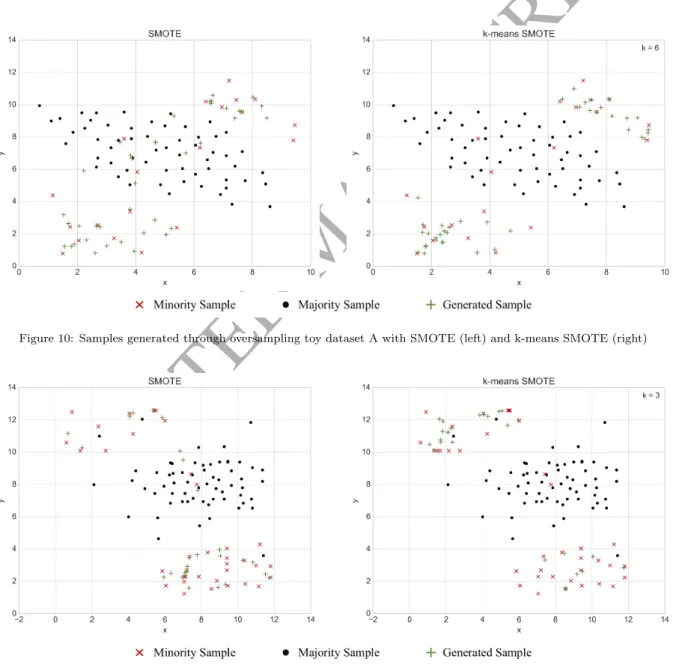
Using two-dimensional toy datasets, it is possible to illustrate how k-means SMOTE may improve the results attained by plain SMOTE. Figures 10 to 14 show the result of applying both methods to simple binary datasets with two to three distinct, albeit slightly noisy, clusters. For all datasets, we observe that SMOTE generates minority samples within majority clusters or directly on the class border. In contrast, the proposed method avoids data generation outside of minority clusters. Particularly figures 13 and 14 exemplify how overlapping class areas are not subject to data generation as they are deemed unsafe. Illustrating the suggested technique’s ability to rebalance within classes, figure 11 shows that SMOTE is inclined to generate most samples in the already dense cluster on the bottom right. In contrast, k-means SMOTE recognizes that the cluster on the top left is sparsely populated and focuses data generation there. Overall, the toy datasets demonstrate that the proposed method is apt to achieve balance between and within classes, while at the same time avoiding noise generation.
The discussed results are based on 5-fold cross-validation with five repetitions, using tests to assure statistical significance. Mean ranking results show that oversampling using k-means SMOTE improves the performance of different evaluated classifiers on imbalanced data. In addition, the proposed oversampler dominates all evaluated oversampling methods in mean rankings regardless of the classifier. Studying absolute gains of the proposed algorithm compared to the baseline method, it is found that all classifiers used in the study benefit from the clustering and sample distribution procedure of k-means SMOTE. Additionally, results of classifying almost any evaluated dataset could be improved by applying the proposed method. Generally, classification problems which are neither very easy nor very difficult profit most, allowing significant score increases of up to 0.3. Lastly, it is found that the number of false positives, which are regarded as an indicator of noise generation, can be effectively reduced by the suggested oversampling technique. Overall it is concluded that k-means SMOTE is effective in generating samples which aid classifiers in the presence of imbalance.
6. Conclusion
Imbalanced data poses a difficult task for many classification algorithms. Resampling training data toward a more balanced distribution is an effective way to combat this issue independently of the choice of the classifier.
ACCEPTED MANUSCRIPT
However, balancing classes by merely duplicating minority class instances encourages overfitting, which in turn degrades the model’s performance on unseen data. Techniques which generate artificial samples, on the other hand, often suffer from a tendency to generate noisy samples, impeding the inference of class boundaries. Moreover, most existing oversamplers do not counteract imbalances within the minority class, which is often a major issue when classifying class-imbalanced datasets. For oversampling to effectively aid classifiers, the amplification of noise should be avoided by detecting safe areas of the input space where class regions do not overlap. Additionally, any imbalance within the minority class should be identified and samples are to be generated as to level the distribution.
The proposed method achieves these properties by clustering the data using k-means, allowing to focus data generation on crucial areas of the input space. A high ratio of minority observations is used as an indicator that a cluster is a safe area. Oversampling only safe clusters enables k-means SMOTE to avoid noise generation. Furthermore, the average distance among a cluster’s minority samples is used to discover sparse areas. Sparse minority clusters are assigned more synthetic samples, which alleviates within-class imbalance. Finally, overfitting is discouraged by generating genuinely new observations using SMOTE rather than replicating existing ones.
Empirical results show that training various types of classifiers using data oversampled with k-means SMOTE leads to better classification results than training with unmodified, imbalanced data. More importantly, the proposed method consistently outperforms the most widely available oversampling techniques such as SMOTE, borderline-SMOTE, and random oversampling. The biggest gains appear to be achieved in clas-sification problems which are neither extremely difficult nor extremely simple. Finally, the evaluation of the experiments conducted shows that the proposed technique effectively reduces noise generation, which is crucial in many applications. The results are statistically robust and apply to various metrics suited for the evaluation of imbalanced data classification.
The effectiveness of the algorithm is accomplished without high complexity. The method’s components, k-means clustering and SMOTE oversampling, are simple and readily available in many programming lan-guages, so that practitioners and researchers may easily implement and use the proposed method in their preferred environment. Further facilitating practical use, an implementation of k-means SMOTE in the Python programming language is made available (see https://github.com/felix-last/kmeans_smote) based on the imbalanced-learn framework [30].
A prevalent issue in classification tasks, data imbalance is exhibited naturally in many important real-world applications. As the proposed oversampler can be applied to rebalance any dataset and independently of the chosen classifier, its potential impact is substantial. Among others, k-means SMOTE may, therefore, contribute to the prevention of credit card fraud, the diagnosis of diseases, as well as the detection of abnormalities in environmental observations.
Future work may consequently focus on applying k-means SMOTE to various other real-world problems. Additionally, finding optimal values of k and other hyperparameters is yet to be guided by rules of thumb, which could be deducted from further analyses of the relationship between optimal hyperparameters for a given dataset and the dataset’s properties.
References
[1] J. Alcal´a-Fdez, A. Fern´andez, J. Luengo, J. Derrac, S. Garc´ıa, L. S´anchez, F. Herrera, Keel data-mining software tool: data set repository, integration of algorithms and experimental analysis framework, Journal of Multiple-Valued Logic & Soft Computing 17.
[2] G. E. A. P. A. Batista, R. C. Prati, M. C. Monard, A Study of the Behavior of Several Methods for Balancing Machine Learning Training Data, ACM SIGKDD Explorations Newsletter 6 (1) (2004) 20–29, ISSN 1931-0145, doi: 10.1145/1007730.1007735 .
[3] C. Bunkhumpornpat, K. Sinapiromsaran, C. Lursinsap, Safe-level-SMOTE: Safe-level-synthetic minor-ity over-sampling technique for handling the class imbalanced problem, in: Lecture Notes in Computer
ACCEPTED MANUSCRIPT
Science (including subseries Lecture Notes in Artificial Intelligence and Lecture Notes in Bioinformatics), vol. 5476 LNAI, ISBN 3642013066, 475–482, doi: 10.1007/978-3-642-01307-2 43 , 2009.
[4] N. V. Chawla, K. W. Bowyer, L. O. Hall, W. P. Kegelmeyer, SMOTE: Synthetic minority over-sampling technique, Journal of Artificial Intelligence Research 16 (2002) 321–357, ISSN 10769757, doi: 10.1613/ jair.953 .
[5] N. V. Chawla, D. A. Cieslak, L. O. Hall, A. Joshi, Automatically countering imbalance and its empirical relationship to cost, Data Mining and Knowledge Discovery 17 (2) (2008) 225–252, ISSN 1384-5810, 1573-756X, doi: 10.1007/s10618-008-0087-0 .
[6] N. V. Chawla, N. Japkowicz, P. Drive, Editorial: Special Issue on Learning from Imbalanced Data Sets, ACM SIGKDD Explorations Newsletter 6 (1) (2004) 1–6, ISSN 1931-0145, doi: 10.1145/1007730. 1007733 .
[7] D. A. Cieslak, N. V. Chawla, A. Striegel, Combating imbalance in network intrusion datasets, in: IEEE International Conference on Granular Computing, 2006, IEEE, ISBN 1-4244-0134-8, 732–737, doi: 10.1109/GRC.2006.1635905 , 2006.
[8] D. A. Cieslak, T. R. Hoens, N. V. Chawla, W. P. Kegelmeyer, Hellinger distance decision trees are robust and skew-insensitive, Data Mining and Knowledge Discovery 24 (1) (2012) 136–158, doi: 10.1007/s10618-011-0222-1 .
[9] J. Demˇsar, Statistical comparisons of classifiers over multiple data sets, Journal of Machine learning research 7 (Jan) (2006) 1–30.
[10] P. Domingos, MetaCost: A General Method for Making Classifiers Cost-Sensitive, in: Proceedings of the 5th International Conference on Knowledge Discovery and Data Mining, 155–164, doi: 10.1145/ 312129.312220 , 1999.
[11] G. Douzas, F. Bacao, Self-Organizing Map Oversampling (SOMO) for imbalanced data set learning, Expert Systems with Applications 82 (2017) 40–52, ISSN 09574174, doi: 10.1016/j.eswa.2017.03.073 .
[12] J. F. D´ıez-Pastor, J. J. Rodr´ıguez, C. I. Garc´ıa-Osorio, L. I. Kuncheva, Diversity techniques improve the performance of the best imbalance learning ensembles, Information Sciences 325 (2015) 98–117, ISSN 0020-0255, doi: 10.1016/j.ins.2015.07.025 .
[13] A. Estabrooks, T. Jo, N. Japkowicz, A multiple resampling method for learning from imbalanced data sets, Computational intelligence 20 (1) (2004) 18–36, ISSN 1467-8640, doi: 10.1111/j.0824-7935.2004. t01-1-00228.x .
[14] A. Fern´andez, V. L´opez, M. Galar, M. J. Del Jesus, F. Herrera, Analysing the classification of imbal-anced data-sets with multiple classes: Binarization techniques and ad-hoc approaches, Knowledge-Based Systems 42 (2013) 97–110, ISSN 09507051, doi: 10.1016/j.knosys.2013.01.018 .
[15] E. Fix, J. Hodges Jr., Discriminatory analysis - nonparametric discrimination: Consistency properties, 1951.
[16] J. H. Friedman, Greedy function approximation: A gradient boosting machine, Annals of Statistics 29 (5) (2001) 1189–1232, ISSN 00905364, doi: 10.1214/aos/1013203451 .
[17] M. Friedman, The Use of Ranks to Avoid the Assumption of Normality Implicit in the Analysis of Variance, Journal of the American Statistical Association 32 (200) (1937) 675, ISSN 01621459, doi: 10.2307/2279372 .
[18] M. Galar, A. Fernandez, E. Barrenechea, H. Bustince, F. Herrera, A review on ensembles for the class imbalance problem: Bagging-, boosting-, and hybrid-based approaches, doi: 10.1109/TSMCC.2011. 2161285 , 2012.
ACCEPTED MANUSCRIPT
[19] M. Galar, A. Fern´andez, E. Barrenechea, H. Bustince, F. Herrera, Ordering-based pruning for improving the performance of ensembles of classifiers in the framework of imbalanced datasets, Information Sciences 354 (2016) 178–196, ISSN 0020-0255, doi: 10.1016/j.ins.2016.02.056 .
[20] I. Guyon, Design of experiments of the NIPS 2003 variable selection benchmark, 2003.
[21] H. Han, W.-Y. Wang, B.-H. Mao, Borderline-SMOTE: A New Over-Sampling Method in Imbalanced Data Sets Learning, Advances in intelligent computing 17 (12) (2005) 878–887, ISSN 1941-0506, doi: 10.1007/11538059 91 .
[22] D. M. Hawkins, The problem of overfitting, Journal of chemical information and computer sciences 44 (1) (2004) 1–12, doi: 10.1002/chin.200419274 .
[23] H. He, E. A. Garcia, Learning from imbalanced data, IEEE Transactions on Knowledge and Data Engineering 21 (9) (2009) 1263–1284, ISSN 10414347, doi: 10.1109/TKDE.2008.239 .
[24] S. Holm, A Simple Sequentially Rejective Multiple Test Procedure, Scandinavian Journal of Statistics 6 (2) (1979) 65–70, ISSN 03036898, 14679469.
[25] R. C. Holte, L. Acker, B. W. Porter, et al., Concept Learning and the Problem of Small Disjuncts, in: IJCAI, vol. 89, 813–818, 1989.
[26] N. Japkowicz, Assessment Metrics for Imbalanced Learning, in: H. He, Y. Ma (Eds.), Imbalanced learning, John Wiley & Sons, 187–206, doi: 10.1002/9781118646106.ch8 , 2013.
[27] T. Jo, N. Japkowicz, Class imbalances versus small disjuncts, ACM SIGKDD Explorations Newsletter 6 (1) (2004) 40–49, ISSN 1931-0145.
[28] S. Kotsiantis, D. Kanellopoulos, P. Pintelas, Handling imbalanced datasets: A review, Science 30 (1) (2006) 25–36, ISSN 14337851, doi: 10.1007/978-0-387-09823-4 45 .
[29] S. Kotsiantis, P. Pintelas, D. Anyfantis, M. Karagiannopoulos, Robustness of learning techniques in handling class noise in imbalanced datasets, doi: 10.1007/978-0-387-74161-1 3 , 2007.
[30] G. Lemaˆıtre, F. Nogueira, C. K. Aridas, Imbalanced-learn: A Python Toolbox to Tackle the Curse of Imbalanced Datasets in Machine Learning, Journal of Machine Learning Research 18 (17) (2017) 1–5. [31] M. Lichman, UCI Machine Learning Repository, 2013.
[32] W.-C. Lin, C.-F. Tsai, Y.-H. Hu, J.-S. Jhang, Clustering-based undersampling in class-imbalanced data, Information Sciences 409-410 (2017) 17–26, ISSN 0020-0255, doi: 10.1016/j.ins.2017.05.008 . [33] L. Ma, S. Fan, CURE-SMOTE algorithm and hybrid algorithm for feature selection and parameter
optimization based on random forests, BMC bioinformatics 18 (1) (2017) 169, ISSN 1471-2105, doi: 10.1186/s12859-017-1578-z .
[34] J. MacQueen, Some methods for classification and analysis of multivariate observations, in: Proceedings of the fifth Berkeley symposium on mathematical statistics and probability, vol. 1, 281–297, 1967. [35] P. McCullagh, Generalized linear models, European Journal of Operational Research 16 (3) (1984)
285–292, doi: 10.1016/0377-2217(84)90282-0 .
[36] I. Nekooeimehr, S. K. Lai-Yuen, Adaptive semi-unsupervised weighted oversampling (A-SUWO) for imbalanced datasets, Expert Systems with Applications 46 (2016) 405–416, ISSN 09574174, doi: 10.1016/j.eswa.2015.10.031 .
[37] A. Nickerson, N. Japkowicz, E. E. Milios, Using Unsupervised Learning to Guide Resampling in Imbal-anced Data Sets, in: AISTATS, 261–265, 2001.
ACCEPTED MANUSCRIPT
[38] F. Pedregosa, G. Varoquaux, A. Gramfort, V. Michel, B. Thirion, O. Grisel, M. Blondel, P. Prettenhofer, R. Weiss, V. Dubourg, J. Vanderplas, A. Passos, D. Cournapeau, M. Brucher, M. Perrot, E. Duchesnay, Scikit-learn: Machine Learning in Python, Journal of Machine learning research 12 (2011) 2825–2830. [39] R. C. Prati, G. Batista, M. C. Monard, Learning with class skews and small disjuncts, in: SBIA,
296–306, doi: 10.1007/978-3-540-28645-5 30 , 2004.
[40] F. Provost, Machine learning from imbalanced data sets 101, in: Proceedings of the AAAI’2000 workshop on imbalanced data sets, vol. 68, AAAI Press, 1–3, 2000.
[41] W. A. Rivera, Noise Reduction A Priori Synthetic Over-Sampling for class imbalanced data sets, Infor-mation Sciences 408 (2017) 146–161, ISSN 0020-0255, doi: 10.1016/j.ins.2017.04.046 .
[42] M. S. Santos, P. H. Abreu, P. J. Garc´ıa-Laencina, A. Sim˜ao, A. Carvalho, A new cluster-based over-sampling method for improving survival prediction of hepatocellular carcinoma patients, Journal of biomedical informatics 58 (2015) 49–59, ISSN 1532-0480, doi: 10.1016/j.jbi.2015.09.012 .
[43] D. Sculley, Web-scale k-means clustering, in: Proceedings of the 19th international conference on World wide web, ACM, 1772690, ISBN 978-1-60558-799-8, 1177–1178, doi: 10.1145/1772690.1772862 , 2010. [44] J. Song, X. Huang, S. Qin, Q. Song, A bi-directional sampling based on K-means method for imbalance text classification, in: International Conference on Computer and Information Science (ICIS), 2016 IEEE/ACIS 15th, 1–5, doi: 10.1109/icis.2016.7550920 , 2016.
[45] J. A. S´aez, J. Luengo, J. Stefanowski, F. Herrera, SMOTE–IPF: Addressing the noisy and borderline examples problem in imbalanced classification by a re-sampling method with filtering, Information Sciences 291 (2015) 184–203, ISSN 0020-0255, doi: 10.1016/j.ins.2014.08.051 .
[46] J. Vanhoeyveld, D. Martens, Imbalanced classification in sparse and large behaviour datasets, Data Min-ing and Knowledge Discovery (2017) 1–58ISSN 1384-5810, 1573-756X, doi: 10.1007/s10618-017-0517-y
.
[47] G. M. Weiss, K. McCarthy, B. Zabar, Cost-sensitive learning vs. sampling: Which is best for handling unbalanced classes with unequal error costs?, DMIN 7 (2007) 35–41.
[48] J. Wu, H. Xiong, J. Chen, COG: local decomposition for rare class analysis, Data Mining and Knowledge Discovery 20 (2) (2010) 191–220, doi: 10.1007/s10618-009-0146-1 .
[49] B. Zhu, B. Baesens, S. K. L. M. vanden Broucke, An empirical comparison of techniques for the class imbalance problem in churn prediction, Information Sciences 408 (2017) 84–99, ISSN 0020-0255, doi: 10.1016/j.ins.2017.04.015 .
ACCEPTED MANUSCRIPT
Figure 8: Performance of KNN classifier trained on different datasets oversampled with SMOTE (left) and k-means SMOTE (right) ordered by AUPRC
ACCEPTED MANUSCRIPT
Figure 9: Relative reduction of false positives compared to SMOTE ordered from highest to lowest average reduction. A high percentage indicates that the proposed method generates fewer minority samples in majority regions than the baseline method.
Figure 10: Samples generated through oversampling toy dataset A with SMOTE (left) and k-means SMOTE (right)
ACCEPTED MANUSCRIPT
Figure 12: Samples generated through oversampling toy dataset C with SMOTE and k-means SMOTE