Monte Carlo simulations of ionization chamber perturbation factors in proton beams

UNIVERSIDADE DE LISBOA

FACULDADE DE CIÊNCIAS

DEPARTAMENTO DE FÍSICA

Monte Carlo Simulations of Ionization Chamber

Perturbation Factors in Proton Beams

Daniela Botnariuc

Mestrado Integrado em Engenharia Biomédica e Biofísica

Perfil em Radiações em Diagnóstico e Terapia

Dissertação orientada por:

Prof. Dr. Luís Peralta

Dr. Ana Mónica Lourenço

A

CKNOWLEDGEMENTS

First, I would like to thank Prof Gary Royle for giving me the opportunity to become part of the amazing proton therapy groups at University College London (UCL) and the National Physical Laboratory (NPL). I am specially grateful to my supervisor, Dr Ana M´onica Lourenc¸o (UCL and NPL), who supported me everyday for a year and without whom this project would have not happened. To Ana M´onica, a huge thank you for being available whenever I had any questions, for the long discussions about protons, electrons and stopping powers, for her priceless guidance, help and friendship. I would also like to express my gratitude to Prof Lu´ıs Peralta, Faculty of Sciences of the University of Lisbon (FCUL), for his patience during poor quality Skype calls, for all his suggestions and advice. A sincere thank you for everything I have learned from him during the past years in the classroom and lab but, most importantly, for passing on the passion for radiation and dosimetry.

I would like to acknowledge everyone in the Medical Radiation groups at NPL. To David Shipley, for helping me to solve my recurring IT problems and to Hugo Palmans, for discussing Monte Carlo and dosimetry problems related to my simulations. To Russell Thomas, for his cheerful mood. I couldn’t be more grateful for the opportunities given to me during my stay at NPL. I have had the chance to participate in the 5th_{edition of Proton Physics Research and}

Implementation Group (PPRIG) workshop. I am also thankful for the unique opportunity to take part in experiments at Paul Scherrer Institut (PSI), in Switzerland and at The Christie NHS Foundation Trust - a high-energy proton beam facility in the UK.

An acknowledgement is addressed to Erasmus for making this internship easier from a financial point of view. I would also like to acknowledge the use of the UCL Myriad High Throughput Computing Facility (Myriad@UCL) and the UCL Legion High Performance Computing Facility (Legion@UCL), and associated support services, in the completion of this work. A genuine thank you to the FLUKA mailing list for answering to all my questions about the code.

I am really grateful for the people I have met in London and made this internship an amazing time of my life. A huge thank you to the Succulent Squad, for offering me a dead succulent and sharing the hall with me everyday. To Hannah, for always having a good story to tell and for cheering me up every time I needed. To Reem and Charles, for inspiring me with awesome science. A kind and special thank you to Michael, for correcting all the commas in this dissertation and for always being there for me. A big thank you to my fittest friends in the world, Inˆes and Beatriz, for always being online for me and to Bruna, for her longtime friendship.

A loving thank you to my family, especially my mum and dad, for the continuous support, love and encouragement throughout my life. To my brother and Nicole, for not forgetting to send me photos and videos of my nephew. Thank you all for always believing in me.

A

BSTRACT

Currently, user reference instruments used in proton dosimetry (proton beam quality, Q) are calibrated at Primary Standard Dosimetry Laboratories (PSDL) in Cobalt-60 beams (beam quality Q0). The difference in the beam qualities

is taken into account in the calculation of absorbed dose to water, Dwater,Q, by introducing the beam quality correction

factor, kQ,Q0. In the analytical calculation of kQ,Q0, all available protocols for reference dosimetry in proton therapy assume ionization chamber perturbation factors, pQ, which account for the non-water equivalence of the air cavity and

entrance window of these detectors, to be unity. This amounts to an uncertainty in the determination of Dwater,Qof

4.6%. This project aimed to determine accurately ionization chamber perturbation factors for the PTW-34070 Bragg PeakR _{chamber in narrow mono-energetic proton beams of 60 MeV, 150 MeV and 250 MeV, and for the PTW-34001} RoosR _{chamber in a spread-out Bragg peak, using FLUKA Monte Carlo code. The influence of different secondary} charged particles on pQwas studied, especially that of secondary electrons, which has not been studied before.

The computation of ionization chambers response is sensitive to boundary crossing artifacts, as particles travel between multiple regions with varying densities. Transport algorithms were validated in FLUKA by performing a Fano cavity test for a plane-parallel ionization chamber, for low-energy protons. FLUKA passed the Fano test within 0.1% accuracy.

Ionization chamber perturbation factors were calculated by simulating different geometries of the two chambers, using the same transport parameters that were validated in the Fano test. For the PTW-34070 Bragg PeakR _{chamber the} perturbation introduced by the air cavity was close to unity for all proton initial energies. Contrary, the presence of the chamber’s wall resulted in perturbations in dose up to 1%. Overall, pQdiffered from unity by approximately 1%. The

simulation of ionization chamber perturbation factors in the modulated beam showed to be extremely time consuming thus, it was not possible to obtain significant results with the available resources.

Ionization chamber perturbation factors can amount to a correction of 1% in high-energy mono-energetic beams, when all secondary charged particles were transported. These factors must be calculated for all ionization chambers used in proton dosimetry and accounted in the calculation of the kQ,Q0. Further investigations must consider the calculation of ionization chamber perturbation factors in modulated beams.

R

ESUMO

A maior motivac¸˜ao em radioterapia para o tratamento de cancro passa por diminuir a dose administrada a tecidos saud´aveis, mantendo ou aumentando a dose depositada no tumor. Ao longo dos anos, in´umeros avanc¸os tecnol´ogicos permitiram ir ao encontro desse objetivo, tais como: a computarizac¸˜ao e automatizac¸˜ao dos sistemas de planeamento do tratatmento, o desenvolvimento de t´ecnicas de imagem avanc¸adas que permitem uma localizac¸˜ao rigorosa do tumor, assim como a introduc¸˜ao de novos tipos de radiac¸˜ao com caracter´ısticas de deposic¸˜ao de dose mais favor´aveis em comparac¸˜ao com aquela obtida tradicionalmente com radiac¸˜ao-X. O uso de prot˜oes em radioterapia apresenta a vantagem destas part´ıculas pararem totalmente nos tecidos, protegendo assim os ´org˜aos a seguir ao alvo de irradiac¸˜ao. Ao atravessarem um meio, taxa de perda de energia dos prot˜oes aumenta `a medida que estes ficam menos energ´eticos, depositando um m´aximo de energia, designada a regi˜ao do pico de Bragg, antes de perderam toda a sua energia, pararando completamente. O alcance dos prot˜oes pode ser manipulado atrav´es da modulac¸˜ao da sua energia inicial de modo a que o pico de Bragg coincida com a regi˜ao do tumor. Clinicamente, a combinac¸˜ao de feixes de energias diferentes produz uma regi˜ao de dose uniforme em profundidade, designada por spread-out Bragg peak (SOBP).

Independentemente do tipo de radiac¸˜ao, a dose deve ser fornecida ao volume alvo com uma incerteza na ordem dos 5%, no intervalo de confianc¸a de 95%. Esta incerteza deve ser entendida como a incerteza global que inclui todas as fontes de incerteza poss´ıveis, como as que advˆem do posicionamento do paciente, do planeamento do tratamento, da entrega de radiac¸˜ao, de procedimentos de calibrac¸˜ao dos instrumentos utilizados, etc. No geral, para ter um m´aximo de 5% de incerteza global, a incerteza dosim´etrica deve contribuir com aproximadamente 1%. Todas as unidades de radioterapia devem assegurar que aos pacientes s˜ao administradas doses com n´ıveis de incerteza internacionalmente aceites. De forma a obter uniformidade no campo da dosimetria, todos os instrumentos de referˆencia de medic¸˜ao da dose devem ser rastre´aveis a Laborat´orios de Dosimetria de Padr˜oes Prim´arios (PSDL).

Este projeto foi desenvolvido na ´area da dosimetria de prot˜oes e teve lugar na University College London (UCL) e no Laborat´orio de Dosimetria de Padr˜oes Prim´arios - o Laborat´orio Nacional de F´ısica (NPL) - no Reino Unido. Em dosimetria, a grandeza de interesse ´e a dose absorvida em ´agua. Atualmente, os PSDL n˜ao possuem feixes de prot˜oes (qualidade de feixe Q) nas suas instalac¸˜oes. Por esta raz˜ao, a calibrac¸˜ao dos intrumentos de referˆencia dos centros de prot˜oes, geralmente cˆamaras de ionizac¸˜ao, ´e feita em feixes de Cobalto-60 (qualidade de feixe de referˆencia Q0).

Devido ao facto da calibrac¸˜ao das cˆamara de ionizac¸˜ao de referˆencia ser feita numa qualidade de feixe diferente daquela na qual os detetores operam, ´e necess´ario introduzir um factor extra, kQ,Q0, no c´alculo da dose absorvida em ´agua, Dwater,Q. Este fator, conhecido como o factor de correc¸˜ao da qualidade de feixe, ´e calculado analiticamente e introduz

uma incerteza de 4.2% na determinac¸˜ao da dose absorvida em ´agua. Esta ´e, de facto, a principal contribuic¸˜ao para a incerteza de Dwater,Qnos feixes de prot˜oes, que por sua vez ´e da ordem dos 4.6%, enquanto que uma incerteza de

apenas 1.5% ´e aplicada em feixes de fot˜oes. De modo a tirar maior partido do potencial que a terapia com prot˜oes apresenta, ´e necess´ario diminuir as incertezas envolvidas na dosimetria de feixes de prot˜oes.

Um dos fatores envolvidos no c´alculo de kQ,Q0 ´e o fator de correc¸˜ao da perturbac¸˜ao das cˆamaras de ionizac¸˜ao, pQ, que corrige a perturbac¸˜ao que a cavidade de ar, pcav, e a parede, pwall, do detetor introduzem na fluˆencia das

part´ıculas do feixe, por n˜ao serem constitu´ıdos por materiais equivalentes `a ´agua. O fator pQ ´e ent˜ao o produto de pcav

por pwall. Nos protocolos de dosimetria de referˆencia atualmente aplicados, pQs˜ao aproximados `a unidade para todos

os modelos de cˆamaras de ionizac¸˜ao, mesmo que haja evidˆencias que estes fatores apresentam uma correc¸˜ao de 1% em feixes de prot˜oes de alta energia. Um dos objetivos deste trabalho foi calcular os fatores de perturbac¸˜ao para a cˆamara de ionizac¸˜ao PTW-34070 Bragg peakR _{em feixes mono-energ´eticos e mono-direcionais de 60 MeV, 150 MeV e 250} MeV. Os fatores pQforam tamb´em calculados para o detetor PTW-34001 RoosR num feixe modulado. Os fatores

de perturbac¸˜ao foram obtidos atrav´es de simulac¸˜oes realizadas no c´odigo de Monte Carlo (MC) FLUKA. Ambos os detetores foram modelados no FLUKA de acordo com as especificac¸˜oes do fabricante. Contrariamente aos estudos feitos anteriormente nesta ´area, o presente trabalho considerou o transporte de todas as part´ıculas secund´arias do feixe, incluindo part´ıculas pesadas carregadas e eletr˜oes.

RESUMO DANIELABOTNARIUC, 2019 A computac¸˜ao da resposta de cˆamaras de ionizac¸˜ao ´e sens´ıvel a artefactos que possam surgir quando as part´ıculas atravessam m´ultiplas regi˜oes de densidades distintas. De facto, estas s˜ao transportadas da regi˜ao que corresponde `a parede da cˆamara de ionizac¸˜ao, que tem uma densidade semelhante `a da grafite, para uma cavidade de ar, que tem uma densidade mil vezes inferior. De modo a evitar artefactos nas simulac¸˜oes, os parˆametros de transporte das part´ıculas no FLUKA tais como a energia perdida num passo de hist´oria condensada (CH), o c´alculo das secc¸˜oes eficazes, o tamanho do passo, devem ser otimizados atrav´es de um teste de auto-consistˆencia (teste de Fano), que ´e suportado pelo teorema de Fano. Este teorema afirma que, em condic¸˜oes de equil´ıbrio de part´ıculas carregadas (CPE), a fluˆencia das part´ıculas carregadas ´e independente de variac¸˜oes de densidade de ponto em ponto, considerando que as secc¸˜oes eficazes s˜ao uniformes em todo o fantoma simulado. Uma forma de implementar este teorema ´e simular uma distribuic¸˜ao uniforme de part´ıculas por unidade de massa num fantoma cujas regi˜oes tenham a mesma composic¸˜ao molecular mas densidades diferentes. O c´odigo de MC passar´a o teste se a dose nas diferentes regi˜oes do fantoma for uniforme.

O teste de Fano foi realizado para otimizar o transporte de part´ıculas no FLUKA num feixe de prot˜oes a baixas energias (20 MeV), para a cˆamara de ionizac¸˜ao PTW-34001 RoosR_{. Para implementar o teste de Fano, a cˆamara de} ionizac¸˜ao foi simulada num fantoma de ´agua em que a todas as regi˜oes do detetor foi atribu´ıdo o mesmo material, neste caso ´agua, de forma a que as propriedades at´omicas sejam uniformes em toda a geometria, mantendo as suas densidades originais. A fonte homog´enea de prot˜oes foi obtida no FLUKA atrav´es de uma rotina modificada do ficheiro ”source.f” em que o n´umero de part´ıculas geradas em cada regi˜ao do fantoma ´e inversamente proporcional `a densidade da regi˜ao. A dose foi calculada em todas as regi˜oes do fantoma. A diferenc¸a relativa nas doses calculadas nas diferentes regi˜oes foi de 0.05%. O FLUKA passou o teste de Fano com uma exatid˜ao de 0.1%.

Os fatores de perturbac¸˜ao para a PTW-34070 Bragg peakR _{e PTW-34001 Roos}R _{foram calculados atrav´es do} c´alculo da dose em diferentes geometrias simplificadas das cˆamaras de ionizac¸˜ao. Sendo a quantidade de interesse a dose absorvida em ´agua, a dose foi primeiramente calculada numa gometria que consistia numa fina camada de ´agua com um raio igual ao da cavidade de ar da cˆamara de ionizac¸˜ao. Seguidamente, a dose foi calculada na cavidade de ar das respetivas cˆamaras de ionizac¸˜ao considerando que o revestimento da cavidade de ar ´e composto pelo material do fantoma - que neste caso foi ´agua. Atrav´es do c´alculo da dose na cavidade de ´agua e na cavidade de ar, ´e poss´ıvel inferir sobre a perturbac¸˜ao introduzida pela presenc¸a das cavidades de ar, pcav, dos dois detetores. Finalmente, a ´ultima

geometria simulada consistiu no modelo original das cˆamaras de ionizac¸˜ao, no qual todos os materiais que comp˜oem as cˆamaras de ionizac¸˜ao foram considerados. Comparando a dose na cavidade de ar quando toda a geometria dos detetores ´e considerada e a dose na geometria que continha apenas a cavidade de ar ´e poss´ıvel obter a perturbac¸˜ao causada pela presenc¸a do revestimento da cavidade de ar, pwall, dos detetores. Para a cˆamara de ionizac¸˜ao PTW-34070 Bragg

peakR_{, p}

cavfoi pr´oximo da unidade para todas as energias dos feixe mono-energ´eticos e mono-direcionais coniderados.

Quanto a pwall, este constituiu uma correc¸˜ao de 1% para feixes de prot˜oes de 250 MeV. De forma geral, quando todas as

part´ıculas secund´arias foram transportadas, pQcontribuiu com uma correc¸˜ao at´e 1% no c´alculo da dose absorvida em

´agua. As simulac¸˜oes dos fatores de perturbac¸˜ao no SOBP mostraram ser extremamente demoradas do ponto de vista computacional, de modo que n˜ao foram obtidos resultados significativos.

De forma a diminuir a incerteza nos kQ,Q0, os fatores de perturbac¸˜ao das cˆamaras de ionizac¸˜ao, p, devem ser calculados considerando o espectro completo das part´ıculas secund´arias em feixes de prot˜oes.

Palavras-chave: Terapia de prot˜oes, dosimetria, fatores de perturbac¸˜ao das cˆamaras de ionizac¸˜ao, teste de Fano, Monte Carlo.

C

ONTENTS

Acknowledgements ii

Abstract iv

Resumo vi

List of Figures x

List of Tables xii

List of Abbreviations xiii

1 Introduction 1

1.1 Radiotherapy . . . 1

1.2 Advantages of proton therapy . . . 2

1.3 The international measurement system – dosimetry metrology . . . 3

1.4 Aim of the work – project overview . . . 5

2 Interactions of Charged-Particles with Matter 6 2.1 Physics Of Particle Interactions . . . 6

2.2 Stopping power . . . 8

2.2.1 The contributions to the total stopping power . . . 8

2.2.2 Restricted electronic stopping power . . . 9

2.3 Nuclear Interactions Of Protons . . . 11

3 Proton Dosimetry 12 3.1 Graphite and water calorimetry . . . 12

3.2 Ionization Chamber Dosimetry . . . 13

3.2.1 Cavity theory . . . 13

3.2.2 Ionization chamber functionality . . . 14

4 Monte Carlo in Radiation Dosimetry 16 4.1 General aspects of Monte Carlo Methods . . . 16

4.1.1 Random number generators . . . 16

4.1.2 Condensed history for charged particle transport . . . 16

4.2 The Fano Test . . . 17

DANIELABOTNARIUC, 2019

5 Materials and Methods 20

5.1 FLUKA Monte Carlo Code . . . 20

5.2 The fano test . . . 20

5.2.1 Phantom geometry and proton source . . . 20

5.2.2 Particle transport physics and scoring . . . 22

5.3 Ionization chamber perturbation correction factors . . . 22

5.3.1 Ionization chamber perturbation factors in narrow mono-energetic proton beams . . . 22

5.3.1.1 The influence of secondary charged particles transport and physics settings . . . . 24

5.3.2 Ionization chamber perturbation factors in a broad modulated beam . . . 26

5.3.3 Determination of the water equivalent thickness of the entrance wall . . . 27

6 Results and Discussion 29 6.1 The Fano Cavity Test . . . 29

6.2 Ionization Chamber Perturbation Corrections Factors . . . 30

6.2.1 Water-to-air stopping power ratios . . . 30

6.2.2 Water equivalent thickness . . . 34

6.2.3 Perturbation factors in narrow mono-energetic proton beams . . . 35

6.2.4 Perturbation factors in a broad modulated beam . . . 39

7 Conclusion 41

L

IST OF

F

IGURES

1.1 Tumour control probability (TCP) and normal tissue complication probability (NTCP) as a function of dose delivered to the patient. . . 1 1.2 Depth-dose distribution curves in water for neutral particles, such as photons (a) and neutrons (b), and

for charged particles, such as electrons (c), protons (d) and carbon-ions (d) [1]. . . 2 1.3 Schematic representation of a Spread-Out Bragg peak (solid line) obtained through the superposition of

individual Bragg peaks (dashed lines) [1]. . . 3 1.4 The calibration sequence for reference and user field dosimeters. . . 4 2.1 Schematic illustration of the different types of interactions of charged particles with a target atom, based

on the comparison of the impact parameter, b, relative to the atomic radius, r. Elastic (a) and inelastic radiative (b) interactions for b ⌧ r, and inelastic hard (c) and soft (d) interactions, b ⇡ r and b r, respectively [2]. . . 7 2.2 Variation of the unrestricted mass electronic stopping power and restricted mass electronic stopping

powers for =10 keV and =100 keV for electrons in water. Adapted from Andreo et al. [2]. . . 10 2.3 Variation of the unrestricted mass electronic stopping power and restricted mass electronic stopping

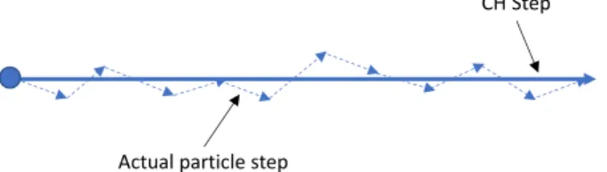
powers for =10 keV and =100 keV for protons in water. . . 11 3.1 Schematic diagram of the composition of a plane-parallel plate ionization chamber. . . 14 4.1 Simulated particle track using the CH technique (solid line) compared to a possible real particle path

(dashed line). . . 16 4.2 Illustration of the chain technique for the calculation of ionization chamber perturbation factors

imple-mented by Lourenc¸o et al. [3] . . . 19 5.1 Schematics of the set up used for the Fano test. All regions of the phantom have water-property materials

and it is divided into the buid-up and CPE regions. The light blue region has air density and it represents the cavity of the ionization chamber; the black region is the chamber’s wall and it was assigned the density of graphite; the blue region represents the water region. The proton sources are represented by the yellow circles. . . 21 5.2 Representation of the PTW-Bragg Peak ionization chamber in sub-figure (a). Simplified schematics of

the detector in (b). The light blue region represent the air cavity with a thickness of 0.2 cm and radius of 4.08 cm. The black region is the chamber’s wall. The entrance wall has a total thickness of 0.347 cm. 23 5.3 Simulation set up for the computation of ionization chamber perturbation correction factors. Water

volume used to score dose-to-water, Dwaterin (a); simulated geometry to determine the dose deposited

in the air cavity, Dairin (b); (c) geometry used to score the dose in the air cavity of the ionization

chamber when its full geometry is considered, Dchamberin (c). twis the thickness of the layer of water

simulated in (a), zw is the depth of measurement and WET is the water-equivalent thickness of the

entrance wall of the chamber. . . 24 5.4 Representation of the PTW-RoosR _{ionization chamber in (a). Simplified schematics of the detector in}

(b). The light blue region represents the air cavity with a thickness of 0.2 cm and radius of 0.78 cm. The black region is the chamber’s wall. The entrance wall has a thickness of 0.113 cm. . . 26 5.5 Simulation set up used for the calculation of the WET. The geometry of the entrance wall of the

correspondent ionization chamber followed by a water region is show in (a) and the water phantom is shown in (b). . . 28

LIST OFFIGURES DANIELABOTNARIUC, 2019 6.1 Depth-dose distribution of the homogeneous mono-directional plane-parallel proton source of 20 MeV

simulated. . . 29

6.2 Depth-dose distribution in the CPE region of the homogeneous mono-directional plane-parallel proton source of 20 MeV simulated. . . 29

6.3 Dose distribution along the x and z axis of the water-property phantom. . . 30

6.4 Restricted and unrestricted mass stopping powers in water for protons. . . 32

6.5 Comparison of the unrestricted mass total stopping power for electrons in water from NIST database and from the thin layer approach. . . 32

6.6 Ratio of the unrestricted mass total stopping powers obtained with FLUKA script to the unrestricted mass total stopping powers from NIST for electrons in water. . . 33

6.7 Bragg-Gray (orange and blue points) and Spencer-Attix (black points) water-to air stopping power ratios for proton beams of initial energies of 60 MeV, 150 MeV and 250 MeV when considering the transport of different particles. . . 34

6.8 The curve in blue is the depth-dose distribution of a 60 MeV proton beam simulated in the entrance window of the PTW- Bragg Peak chamber followed by the water phantom. The orange curve represents the depth-dose distribution in the water phantom for the same beam. The water-equivalent thickness (W ET ) of the entrance window of the chamber is the difference between the range at 80% dose of the two curves. . . 35

6.9 2-dimensional dose distribution in the geometry used to score dose to water (a), in the geometry simulated to determine the dose in the air cavity (b) and in the geometry used to score the dose in the air cavity of the chamber when its full geometry is considered (c). . . 37

6.10 Ionization chamber perturbation correction factors as a function of the beam energy when all charged particles are transported (black points), electrons are discarded (blue points) and nuclear interactions and electrons are discarded (orange points). pcavare represented in (a); pwallare represented in (b) and the total perturbation, pQ, is shown in (c). . . 38

6.11 Depth-dose distribution of the SOBP simulated in the water phantom. . . 39

6.12 Depth-dose distribution of the flat region of the SOBP simulated in the water phantom. . . 40

L

IST OF

T

ABLES

6.1 Dose values scored in the regions of the geometry simulated with different densities. The represented uncertainties are of type A. . . 30

LIST OFABBREVIATIONS DANIELABOTNARIUC, 2019

L

IST OF

A

BBREVIATIONS

BG Bragg-Gray

CH Condensed History

CPE Charged particle equilibrium MC Monte Carlo

NPL National Physical Laboratory

PSDL Primary Standards Dosimetry Laboratory RNG Random Number Generator

SSDL Secondary Standards Dosimetry Laboratory

SA Spencer-Attix

SOBP Sprea-out Bragg peak WET Water-equivalent thickness

1 I

NTRODUCTION

1.1 R

As reported by the World Health Organization, cancer is the second leading cause of death in the world and it was responsible for an estimated 9.6 million deaths in 2018 [4, 5]. In the initial stage of cancer development, the tumour is commonly confined to a specific anatomical tissue, in which it starts growing. While the disease is still well localized, surgical procedure or radiation therapy is the elected approach for treatment. In case the tumour is in close proximity to a vital organ or completely inaccessible with surgery, radiation therapy will be the preferred method. As the disease progresses, cancers can spread from their site of origin to nearby lymph nodes and start growing into other tissues or organs, evolving to metastases. To treat metastatic cancers, the suggested approaches are chemotherapy and immunotherapy, which are systemic methods. All cancer treatment techniques just described can be performed either as single treatments or, more commonly, in combination. This project will focus on radiation therapy for tumour eradication using protons.

In general, radiation can interact with biological tissue and cause direct or indirect damage to the genetic material (deoxyribonucleic acid, DNA). Direct damage occurs with the direct ionisation of the DNA strand by radiation whereas indirect damage occurs by ionising water molecules, which creates reactive free radicals that can provoke harmful intracellular reactions. Both damage types can lead to lethal reactions in the cell and the likelihood of cell death increases with increasing radiation dose. The major drawback in radiotherapy is that radiation affects both malignant cells and healthy tissues, thus, it is necessary to find the correct compromise between tumour eradication and healthy tissue damage [6].

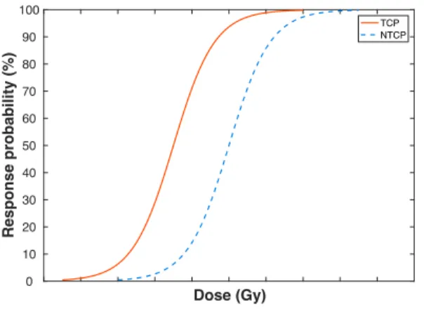
Radiation killing of single cells is stochastic since it depends on the occurrence of individual ionizing events. However, if a tumour mass or organ is considered, the effect of radiation is deterministic, i.e. there is a dose threshold bellow which no clinical response will be observed and a dose above which the effect will be observed in every individual. This is illustrated in figure 1.1 where tumour control (solid line) and healthy tissue damage (dashed line) probabilities are presented as a function of dose. Tumours that can be treated with radiotherapy are those in which the tumour control curve appears on the left side of the healthy tissue damage curve. The more separated are these curves, the more effective will be the radiotherapy treatment. Note that both curves are very steep and consequently their dependence in dose is very high. For this reason, the uncertainty in dose delivered to patient should be as small as possible [7].

Dose (Gy) 0 10 20 30 40 50 60 70 80 90 100 Response probability (%) TCP NTCP

Figure 1.1: Tumour control probability (TCP) and normal tissue complication probability (NTCP) as a function of dose delivered to the patient.

The major goal and motivation for research in radiotherapy treatment techniques for cancer is to reduce delivered dose to healthy tissue while maintaining or increasing the dose to the target structure within acceptable uncertainty in order to improve patient outcomes. As recommended by the ICRU Report 24 [8], the absorbed dose to a target volume

1 INTRODUCTION DANIELABOTNARIUC, 2019 in the patient should be delivered with an accuracy of 5% at 95% confidence level. This 5% includes different types of uncertainties, such as the uncertainty from calibration procedures in primary standard laboratories and reference absorbed dose measurements, as well as uncertainties introduced by patient positioning, treatment planning and dose delivery. For optimal treatment of patients, it is critical for dosimetric uncertainties to be as small as possible (around 1%).

1.2 A

Not long after the discovery of x-rays in 1895 [9], ionizing radiation was employed to treat cancer. Since then, research in physics and medicine has contributed to the improvement of radiation therapy and nowadays this is the main option for treatment in oncology [10]. Radiation interacts with matter via atomic and nuclear interactions. The mean energy deposited by the ionizing radiation, d¯", in a mass of material, dm, in such interactions is quantified as absorbed dose, D, and it is expressed in energy (J) absorbed per unit mass (kg) – which has the unit of gray (Gy) [11]:

D = d¯"

dm (1.1)

Over the years, many advances have been made with the main objective of increasing the dose delivered to the tumour whilst sparing surrounding healthy tissues. For instance, imaging techniques are more precise, allowing a more accurate tumour localisation, the treatment planning systems became computerized and new radiation types were introduced because of more favourable dose deposition characteristics. The advantage of proton therapy for tumour eradication relies on the finite range of these particles in tissue and it can be understood by comparing depth-dose distributions in water for distinct particles used in radiotherapy.

e

n

C-ion

Figure 1.2: Depth-dose distribution curves in water for neutral particles, such as photons (a) and neutrons (b), and for charged particles, such as electrons (c), protons (d) and carbon-ions (d) [1].

neutrons show a short build-up region followed by an exponential-like decay in dose. As the absorbed dose is directly dependent of the particle fluence (number of particles per unit area), the dose can be seen to decrease exponentially as the fluence falls exponentially due to interactions with matter. For neutral particles, dose is not directly delivered to the medium, instead, these particles will interact in matter and release secondary electrons, which then proceed to deposit their energy in the medium. The secondary electrons will not deposit their energy immediately at the site they were produced and this is why the depth-dose curves show an initial build-up region. This aspect is particularly useful for radiotherapy as it allows one to spare the skin from undesirable high dose depositions. Figures 2 (c), (d) and (e) show characteristic depth-dose distribution curves for charged particles, arranged by increasing mass. Contrary to neutral particles, the fluence of charged particles only decreases slightly with depth. All charged particles lose their energy continuously and the rate of energy loss increases as these slow down, having a maximum energy deposition at the end of their track. The peak in dose is named as Bragg peak and it is sharper the heavier is the particle. The range of the particles and, therefore, the depth of the Bragg peak can be adjusted by varying the initial energy of the beam. One can see that the maximum dose peak for electrons is quite broad due to the small electron mass. For being light particles, these scatter more in matter. For heavier particles such as protons and carbon-ions, the peak is much sharper. This feature is the main advantage of the use of proton over photons in radiotherapy since one can point the maximum dose deposition to a tumour target whilst sparing the tissues behind it. Clinically, if a certain number of proton beams with different energies are produced in the same direction, distinct Bragg peaks will occur, as it is shown by the dashed curves in figure 1.3. The combination of these peaks produces the so-called Spread-Out Bragg peak (SOBP), represented by the solid line. The proton beam is modelled in such a way so that the maximum energy is deposited uniformly across the target volume defined by the dark grey region. For patient treatments, energies between 50 MeV and 250 MeV are used, which allows a penetration in tissue from a few millimetres up tp 40 cm. As the beam stops in tissue, dose is not delivered to healthy tissues located behind the tumour (light grey area), reducing the risks of long-term side effects. This type of therapy is particularly beneficial to children and young adults as their healthy tissues are still in development [1].

Figure 1.3: Schematic representation of a Spread-Out Bragg peak (solid line) obtained through the superposition of individual Bragg peaks (dashed lines) [1].

1.3 T

–

Proton centres and radiotherapy units in general need to ensure that patients undergoing radiation treatment receive doses within internationally accepted levels of accuracy. To accomplish national and international uniformity in dosimetry metrology, user reference instruments should be traceable to Primary Standards either by direct calibration in a Primary Standard Dosimetry Laboratory (PSDL) or, more commonly, in a Secondary Standard Dosimetry Laboratory (SSDL), which in turn is linked to a PSDL. Only a small number of countries in the world are provided by PSDL for radiation

1 INTRODUCTION DANIELABOTNARIUC, 2019 dosimetry so it is impossible for these to calibrate all dosimetry instruments used all over the world. For this reason, countries with national laboratories for primary standards calibrate secondary standards laboratories. The calibration chain for user reference instruments is illustrated in figure 1.4.

Primary Standards

Secondary Standards

Reference

Standards

User Field

Standards

To better understand the calibration chain, it is necessary to distinguish between primary, secondary, reference and user field standards. To begin with, a primary standard is defined as an instrument of the highest metrological quality that allows to determine a unit of a quantity from its definition. The accuracy of a primary standard is established by comparing it with other standards of other institutions at the same level. On the other hand, a secondary standard is an instrument calibrated against a primary standard. The reference standard is defined as an instrument of the highest metrological quality accessible at a given location, from which measurements at that location are derived. Finally, the user field standard is the instrument used for routine measurements in radiotherapy centres, which is calibrated against the reference instrument at the site. In practice, radiotherapy units possess several field dosimeters for daily measurements and only one reference instrument. The reference instrument of the radiotherapy unit is normally sent to a PSDL or a SSDL where it is calibrated. It is important to note that the reference instruments at the PSDL or SSDL may not be directly calibrated against the primary or secondary standard. Instead, PSDLs and SSDLs calibrate hospitals’ reference instruments against their own reference standards (the transfer standards), which in turn is calibrated against primary or secondary devices. This procedure is used because primary and secondary instruments are very sensitive and complex to operate, therefore it is not convenient to handle them often. Transfer standards are, in fact, considered part of the primary standards themselves and this system has proven to be highly consistent throughout the years.

In dosimetry, the quantity of interest is absorbed dose to water since water is the proxy for biological tissue. At PSDLs, the absolute value of this quantity can be determined via three basic techniques, which are calorimetry, chemical dosimetry or ionization dosimetry. At the National Physical Laboratory (NPL) in the United Kingdom, the primary standards of absorbed dose to water are determined using graphite calorimeters and operated in a Cobalt-60 gamma-ray beam quality, as well as in photon and electron beams. Currently, PSDLs do not have access to proton beams in their facilities. Usually, the reference instruments as well as user field instruments are ionization chambers [12].

At NPL, the general calibration chain begins with the direct determination of absorbed dose-to-water from a Cobalt-60 beam (beam quality Q0), Dwater,Q0, using a graphite calorimeter. Afterwards, the exact same dose is delivered by the same beam quality to the reference dosimeter and its reading, MQ0is registered. The absorbed dose-to-water in the absence of the ion chamber, at the reference depth zref in a water phantom, for the beam quality Q0, is related to the

reference dosimeter’s reading through the calibration coefficient of the dosimeter in terms of absorbed dose-to-water for the beam quality Q0, ND,W,Q0, and it is expressed by:

Dwater,Q0= MQ0· ND,w,Q0 (1.2)

As mentioned above, PSDLs have no direct access to a proton beam in their facilities. This means that the reference instruments are calibrated in the reference beam quality, Q0– Cobalt-60 – which is different from the beam quality, Q,

they are meant to operate in, which is, in this case, a proton beam. When two distinct beam qualities are involved, the equation of absorbed dose to water for the beam quality, Q, is given by:

Dwater,Q= MQ· ND,w,Q0· kQ,Q0 (1.3) where MQis the chamber’s reading in the proton beam, ND,w,Q0represents the calibration coefficient of the dosimeter in the reference beam quality Q0referred above and the factor kQ,Q0is the beam quality correction factor which corrects for the different response of the ionization chamber between the user beam quality Q and the calibration beam quality Q0.

The beam quality correction factor can be obtained directly from calorimetry experiments by the ratio of the calibration coefficients in terms of absorbed dose-to-water at the qualities Q and Q0. Because of the lack of proton

beams in PSDLs, kQ,Q0are calculated analytically as: kQ,Q0 =

(Wair/e)Q· (swater,air)Q· pQ

(Wair/e)Q0· (swater,air)Q0· pQ0

(1.4) where Wair/eis the energy required to produce an ion pair, sw,airis the water to air stopping power ratio and p is the

ionization chamber perturbation factor which accounts for the non-water equivalence of the air cavity and the chamber’s wall. The equations (1.3) and (1.4) were first proposed by Hohlfeld [13] in 1988 for high-energy photon beams and established later for proton beams by Medin et al. [14] in 1995. The same methodology is employed in the IAEA TRS-398 code of practice, which is the reference protocol used in proton beams [12].

In proton beams, the beam quality correction factor, kQ,Q0, introduces an uncertainty of 4.2% (k=2) in the determination of absorbed dose-to-water. In fact, this is the main contribution to the uncertainty of Dwater,Q, which is

of the order of 4.6% (k=2), whereas an uncertainty of only 1.5% (k=2) is estimated for photon beams. The quantities that introduce the largest uncertainty in kQ,Q0are swater,airand p [12].

1.4 A

–

The use of proton beams for radiotherapy has expanded in the last few decades. To use this technique to its full potential, uncertainties on reference dosimetry in proton therapy should be improved. This project aims to improve reference dosimetry by minimising the uncertainty in dose calculations caused by the non-water equivalence of the air cavity and entrance window of ionization chambers currently used worldwide in clinical proton therapy facilities. All available protocols for reference dosimetry in proton therapy consider ionization chamber perturbation factors, p, to be unity, although it is known from previous work that these perturbation factors can amount to 1% [15]. This contributes to uncertainties in the determination of absorbed dose-to water which is of the order of 4.6% (k=2) for proton therapy beams, compared to 1.5% (k=2) of uncertainty in photon therapy [12]. Ionization chamber perturbation factors are calculated by considering different geometries of the chamber at water-equivalent depths using FLUKA Monte Carlo (MC) code, which requires the development of code with detailed modelling of these detectors. Moreover, dosimetry calculations within MC codes are very sensitive to artifacts if the correct physics list are not used. The particle transport algorithms, the energy loss along the condensed history (CH) step and the boundary crossing events must be as accurate as possible. Therefore, the MC code used to perform the proposed calculations was evaluated through a self-consistency test, the so called Fano test.

2 INTERACTIONS OF CHARGED-PARTICLES WITH MATTER DANIELABOTNARIUC, 2019

2 I

NTERACTIONS OF

C

HARGED

-P

ARTICLES WITH

M

ATTER

In radiation dosimetry, it is crucial to understand in detail the mechanisms of radiation interactions with matter in order to characterise, as accurate as possible, the energy deposition in a biological tissue [2]. Charged particles have an electric field, thus the process of energy loss for these particles is mainly based on electromagnetic or Coulomb interactions with atomic electrons and nuclei. In addition to electromagnetic interactions between charges, heavy charged particles can occasionally undergo head-on collisions with atomic nuclei (non-elastic nuclear interactions), which alter the beam fluence by changing the nature of the projectile, decreasing the primary beam fluence, and setting secondary particles in motion, discussed in section 2.3.

Electrons and positrons present a mass value much smaller in comparison with other charged particles. This influences the amount of energy transferred in one collision with matter, as well as the scattering angles. For this reason, it is suggested to consider these lighter particles in a different category from charged particles heavier than electrons. Although the aim of this work is to study proton beams, secondaries such as other heavy charged particles and electrons are considered since they result from proton interactions. Thus, an overview of charged particle interactions with matter is presented.

2.1 P

O

P

I

Charged particles interact with atomic electrons and nuclei as they pass through matter. These interactions result in energy losses and scattering of the projectiles along their track and also in excitation and ionization of the atoms in the medium. Each of these interactions is assigned a specific cross section , i.e., the probability of a particular interaction. Charged-particle Coulomb interactions are divided into four categories based upon the relationship between the classical impact parameter b - defined as the distance between the projectile and the atom’s centre - and the atomic radius, r [16]. These four types of interactions are shown in figure 2.1 and the description of each situation is generalised for all charged particles, however, some occur more frequently for either light or heavy particles.

b ⌧ r: Elastic and inelastic radiative interactions

In the cases presented in sub-figures 2.1 (a) and 2.1 (b), the impact parameter, b, is much smaller than the radius, r, of the atom in the medium, which means that the projectile interacts mainly with the atomic nucleus. Electromagnetic interactions of charged particles with the external nuclear field result in either elastic or inelastic scattering. Elastic interactions are the most frequent and are characterized by the deflection of the projectile’s trajectory by the nucleus, especially in high-Z materials. When a beam of particles traverses a slab of material, it diverges due to the particles’ deflection by the atomic nuclei. The lighter is the projectile, the larger are the deflections. In fact, this is the main mechanism by which electrons scatter. However, the scattering angles due to a single collision are typically very small therefore the increasing cross sectional area of the beam is a result of multiple Coulomb scattering (MCS). In order to conserve the momentum in a collision, the projectile loses a small amount of its initial kinetic energy, which is extremely small for the therapeutic energy range, and the target atom does not suffer excitation nor ionization. For example, for heavy charged particles, this type of collision contributes minimally, less than 1%, to the total energy loss, unless for particles with energies below several tens of keV [17].

In contrast, during inelastic radiative interactions, the incident particle may undergo a significant energy loss, with the emission of a x-ray (bremsstrahlung) photon or provoke an excited state in the nucleus. In fact, bremsstrahlung radiation does not occur exclusively upon interactions with the nucleus. This type of radiation can also be emitted upon interactions with the Coulomb field of atomic electrons [18].

For both elastic and inelastic radiative types, the interaction cross section depends on the square of the atomic number (Z2_{) of the target material. Furthermore, the inelastic radiative interaction cross section is inversely proportional}

r b

Projectile

(a) Elastic interaction

b ≪ r

r b

Projectile

(b) Inelastic radiative interaction

b ≪ r

hv

r b

Projectile

(c) Inelastic hard collision

b ≈ r

Ejected 𝛿- ray

r b

Projectile

(d) Inelastic soft collision

b ≫ r

Excited or ejected e-

Figure 2.1: Schematic illustration of the different types of interactions of charged particles with a target atom, based on the comparison of the impact parameter, b, relative to the atomic radius, r. Elastic (a) and inelastic radiative (b) interactions for b ⌧ r, and inelastic hard (c) and soft (d) interactions, b ⇡ r and b r, respectively [2].

particles heavier than electrons or positrons. b ⇡ r: Inelastic hard collision

In the sub-figure 2.1 (c), the impact parameter of the projectile is similar to the atomic radius of the absorber material. In this situation, the charged particle is more likely to interact directly with a single atomic electron, commonly from an inner shell, transferring part of its energy to the electron. Typically, the energy transferred is much larger than the electron’s atomic binding energy, therefore, hard collisions can be approximated as interactions between the charged projectile and a free electron. Upon this interaction, the electron, now referred to as a delta-ray ( -ray), is ejected from the atom with a significant kinetic energy, enough to undergo its own interactions with the medium and to deposit its energy along a different track from the primary charged particle. The probability for inelastic hard collisions between charged particles and electrons is small. The energy loss depends on the type of the incident particle. Light projectiles, for instance, could lose a significant amount of its kinetic energy in this type of interaction.

b r: Inelastic soft collision

Sub-figure 2.1 (d) shows the projectile interacting with the atom as a whole, since the impact parameter of the charged particle is much larger than the atomic radius. These interactions are characterized by small energy transfers and the main resulting effects are excitation and ionization of the atoms in the medium. Even though the energy transferred to the atom is of the order of a few eV, inelastic soft collisions are by far the most frequent, therefore the charged particle could lose around 50% of its kinetic energy to the medium [19]. The energy transferred by a particle undergoing hard and soft collisions are the most impactful mechanisms for energy loss.

2 INTERACTIONS OF CHARGED-PARTICLES WITH MATTER DANIELABOTNARIUC, 2019

2.2 S

Charged particles traversing a medium will undergo the interactions described above with the atoms of the material, losing their energy along their track, until they stop in the medium. The average energy loss, dE, per unit path length, dx, is defined as the linear stopping power, S, of the traversed material and it is expressed in MeV/cm:

S = dE

dx (2.1)

A commonly used quantity is the mass stopping power, (1/⇢)dE/dx, which has units of MeV·cm2_{/g. This}

quantity is usually preferred due to its low dependence on the density of the traversed material [20]. For heavy charged particles, depending on the mechanisms of particles interactions, one can distinguish two components of the total stopping power: electronic (el), also called collision (col), and nuclear (nuc) stopping powers (equation 2.2). The former results from interactions of charged particles with atomic electrons. It includes both inelastic hard and soft collisions and it is the main contribution to the total stopping power. With regards to the nuclear stopping power, it only includes energy losses due to elastic interactions between the projectile and the atomic nuclei of the target, as inelastic radiative interactions are only relevant for electrons and positrons.

1 ⇢ dE dx ! total = 1 ⇢ dE dx ! el 1 ⇢ dE dx ! nuc (2.2) For electrons and positrons, the total stopping power accounts the contribution of the collision (col), also called electronic (el), and the radiative (rad) stopping powers (equation 2.3). The former includes the same type of interactions as described above for heavy charged particles. The radiative stopping power includes all inelastic energy losses in which bremsstrahlung radiation is emitted.

1 ⇢ dE dx ! total = 1 ⇢ dE dx ! col 1 ⇢ dE dx ! rad (2.3)

2.2.1 THE CONTRIBUTIONS TO THE TOTAL STOPPING POWER

The calculation of the energy loss to atomic electrons due to interactions of heavy charged particles and electrons was first introduced by Bohr using classical arguments. This quantity was later extended to quantum mechanics by Bethe, Bloch and others [21].

• Heavy charged particles

For charged particles heavier than electrons and positrons, the nuclear component of the stopping power is negligible, especially for the therapeutic energy range, thus Stotal⇡ Sel. According to the ICRU Report 49, Sel

is calculated as the sum of energy loss due to both hard and soft collisions [17]. This is formulated as follows: 1 ⇢Sel= 4⇡r2 emec2 u 1 2 Z Az 2_· " ln 2mec 2 2 I ! ln(1 2₎ 2 # (2.4) where rerepresents the classical electron radius, mec2the electron rest mass energy, u the atomic mass unit,

is the velocity of the incident charged particle as a fraction of the speed of light ( = v/c), Z/A is the ratio of number of electrons per molecular weight of the medium and z the projectile charge. In the logarithmic factor, I is the mean excitation energy of the medium.

• Electrons and positrons

For electrons, the collision stopping power expression differs from the one presented for heavy particles since the energy loss due to soft collisions has a different formulation for these particles. According to the ICRU Report 37 [18], the mass collision stopping power for electrons is written as follows:

1 ⇢Scol= 2⇡r2 emc2 u 1 2 Z A· " ln E 2 k I2 ! + ln 1 ⌧ 2 ! + F (⌧ ) # (2.5) where Ekis the kinetic energy of the incident electron and ⌧ = Ek/mec2. The function F (⌧) is expressed as:

F (⌧ ) = (1 2)

 1 +⌧

2

8 (2⌧ + 1) ln 2 (2.6)

Contrary to heavy charged particles, when calculating the total stopping power for electrons or positrons, it is important to take into account the radiative component, particularly at higher kinetic energies. The general expression for the mass radiative stopping power is given as:

1

⇢Snuc= Na radE0 (2.7)

where Na represents the number of atoms per unit mass in the traversed medium, radis the cross section

function for bremsstrahlung production, which is a function that depends on Z and also on E0, being E0the

initial total energy of the electron or positron; the function raddepends on the kinetic energy of the light particle

and has different formulations for non-relativistic, relativistic and high-relativistic energy ranges [19].

The most relevant feature in the mass electronic stopping power formulas for both heavy and light charged particles is the inverse dependence on the velocity of the incident particle, . This aspect translates the increase in energy loss as the particle slows down. Several corrections were added to both original formulations later, such as the density effect, ( ), and shell, (C), corrections [22]. The former accounts for polarization effects, specially in solid media and it only becomes relevant at high energies. The shell correction becomes important at low energies, when the velocity of the projectile is lower than the velocity of orbital electrons of the atoms in the medium.

2.2.2 RESTRICTED ELECTRONIC STOPPING POWER

In dosimetry, it is of interest to measure the energy deposited by charged particles in a specific region, usually referred as cavity. The detectors used for these measurements are usually ionization chambers. As mentioned above, the electronic or collision stopping power is the energy loss by charged particles to atomic electrons, Sel, and it includes both hard and

soft collisions. However, -rays ejected in hard collisions could be energetic enough to escape the region of interest and therefore deposit their kinetic energy outside the cavity. Due to this effect, it was introduced a new quantity known as the restricted stopping power, L . The latter does not account for the energy loss by -rays with energies higher than a certain threshold , which is established depending on the cavity size [16]. The original electronic stopping power is now called the unrestricted electronic stopping power and it is larger than the restricted stopping power as it overestimates the energy loss by charged particles as it considers that all -rays deposit their energy locally. Note that it is meaningless to establish a value greater than the maximum energy transferred to an atomic electron in a hard collision, Emax, . The lower the threshold, the larger is the divergence between restricted and unrestricted stopping

powers. As one increases , the disparities become lower and when = Emax, , the restricted stopping power is

2 INTERACTIONS OF CHARGED-PARTICLES WITH MATTER DANIELABOTNARIUC, 2019 Figure 2.2 illustrates the unrestricted mass electronic stopping power (solid line) and the restricted mass electronic stopping powers for thresholds of =10 keV (dotted line) and =100 keV (dashed line) as a function of the kinetic energy of electrons in water. All curves were obtained through Monte Carlo (MC) simulations, using the FLUKA MC code [23, 24]. In order to analyse the discrepancies between unrestricted and restricted stopping powers and the respective threshold values, it is important to have an idea of Emax, . The maximum energy transferred depends on

the incident charged particle. For instance, electrons transfer up to half of their kinetic energy to -rays. This means that for a fixed value of energy transfer , the electron must have a minimum kinetic energy of 2 to produce a -ray. Therefore, for kinetic energies up-to 2 the unrestricted and restricted stopping powers coincide whereas for kinetic energies higher than 2 the restricted stopping power becomes lower. This is shown in figure 2.2 where, for =10 keV and =100 keV, the restricted stopping power starts to diverge from the unrestricted stopping power at 20 keV and 200 keV, respectively.

10-2 10-1 100 101

Electron kinetic energy (MeV)

100 101

Mass electronic stopping power (MeV cm

2/g) Restricted SP: =10 keV Restricted SP: =100 keV Unrestricted SP 20 keV 200 keV

Figure 2.2: Variation of the unrestricted mass electronic stopping power and restricted mass electronic stopping powers for =10 keV and =100 keV for electrons in water. Adapted from Andreo et al. [2].

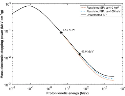
Figure 2.3 shows the same curves as described above for the case of protons. The minimum energy that protons must have in order to produce a 10 keV and a 100 keV -ray is 4.59 MeV and 45.9 MeV respectively. This energy can be calculated according to the following expression:

E = 1

4·

(M + m)2

M· m · Etransf (2.8)

where M = 1.673 ⇥ 10 27_{kg is the proton mass, m = 9.109 ⇥ 10} 31_{kg is the electron mass and E}

transf = , which

is the maximum energy transfer to the electron. For =10 keV and =100 keV, the restricted stopping power starts to diverge from the unrestricted stopping power at 4.59 MeV and 45.9 MeV, respectively.

10-2 10-1 100 101 102 103 104

Proton kinetic energy (MeV)

10-3 10-2 10-1 100

Mass electronic stopping power (MeV cm

2 /g) Restricted SP: =10 keV Restricted SP: =100 keV Unrestricted SP 4.59 MeV 45.9 MeV

Figure 2.3: Variation of the unrestricted mass electronic stopping power and restricted mass electronic stopping powers for =10 keV and =100 keV for protons in water.

2.3 N

I

O

P

In addition to Coulomb interactions with atomic electrons and the nuclear electric field, heavy charged particles may undergo the so called non-elastic nuclear interactions [25]. For the specific case of a proton beam, in such interactions, a proton may enter into the nucleus of a target atom to form an excited system which is later fragmented resulting in secondary particles such as protons, that includes also the primary proton since it is no longer distinguishable, neutrons or lighter fragments of the nucleus. Even though these interactions are considered to be rare when compared to electromagnetic interactions, they are not negligible and must be taken into account. For a 60 MeV proton beam, about 4% of the primary protons are lost before stopping due to non-elastic nuclear interactions [26]. The decline in the number of primary protons is higher as the energy of the beam increases so that, for instance, a 160 MeV proton beam, loses almost 20% of its primary protons in this type of interaction [1]. For a 250 MeV proton beam, the number of primary protons decreases in such a way that the peak-to-plateau ratio of dose decreases by a factor of 40% [27]. Therefore, to perform accurate studies with proton beams it is of great importance to consider non-elastic nuclear interactions and consider the secondary particles generated in these interactions.

The secondary charged particles resulting from non-elastic nuclear interactions could be secondary protons, deutrons, tritons, helions and alphas; from these interactions could also result neutrons as well as gamma rays.

3 PROTON DOSIMETRY DANIELABOTNARIUC, 2019

3 P

ROTON

D

OSIMETRY

The dosimetry field can be divided into absolute and relative dosimetry. The first is characterized as the fundamental measurement of absorbed dose in a medium with a detector, without need for calibration of the detector’s response. The latter derives from the former, which means that relative dosimeters must be calibrated against absolute systems [19]. As mentioned previously, three different techniques are used for absolute dosimetry in PSDL, which are calorimetry, chemical dosimetry and ionization dosimetry. Only calorimetric dosimetry will be discussed in the next section since this is the primary standard method used at NPL for photon and particle beams.

3.1 G

Calorimetric dosimetry is based on measuring the temperature rise in a medium as a result of energy deposition by ionizing radiation. The instrument used for calorimetry measurements is known as a calorimeter and it contains a small cavity, the sensitive volume, in which dose is to be determined. The point of measurement is thermally insulated from the exterior materials and it incorporates a temperature sensor, i.e. a thermistor. When the calorimeter is irradiated, only a fraction of the energy transported by the beam’s particles is transferred and deposited in the medium, resulting in the temperature rise measured. The resulting thermal energy, Q, in the point of measurement is expressed by:

Q = m· c · T (3.1)

where m refers to the mass of the medium, c is the specific heat capacity of the medium expressed in J kg 1_K 1_and

T is the temperature rise in the medium. Assuming that all energy deposited in the calorimeter’s core is converted into heat, the equation above can be rearranged in terms of absorbed dose in the medium:

Q

m = D = c· T (3.2)

In radiation dosimetry, the quantity of interest is absorbed dose to water, so water would be the ideal medium for a calorimetry system. According to NIST, the specific heat capacity of water is 4186 J kg 1_K 1_{. In a radiotherapy}

context, doses of the order of 2 Gy are delivered to patients in each fraction, therefore the rise in temperature in a water calorimeter would be of the order of 0.5 mK. It is undeniable that such a small increase in temperature is extremely hard to measure and this is clearly the major disadvantage of water calorimetry. Water calorimeters are used for absolute dose measurements, but these are not convenient for routine measurements because of their lack of sensitivity and complexity of operation. The difficulty with water calorimeters is due to the high specific heat capacity of water. If water could be replaced by another material with lower specific heat, the temperature rise per unit dose will increase -since, as shown in equation 3.2, T is inversely proportional to c. As an alternative to water, graphite is often used as the medium of interest in calorimetry. According to NIST, the specific heat capacity of graphite is 710 J kg 1_K 1_,

which is about 6 times smaller than that of water, therefore the increase in the medium’s temperature is around 6 times larger. Subsequently, for the same dose of 2 Gy, the rise in temperature in a graphite calorimeter is approximately 2.8 mK. Although this temperature rise is significantly larger and therefore relatively easier to measure than the one for water, graphite is not as tissue equivalent as water, despite having similar atomic numbers. This means that the obtained quantity, which is absorbed dose-to-graphite, needs to be converted into absorbed dose-to-water through conversion factors. The latter introduces larger uncertainties in the determination of absorbed dose-to-water in comparison with water calorimetry [19, 28].

To conclude, some PSDLs use water calorimeters whereas others use graphite calorimeters for absolute dose determination in photon and particle beams. Clearly, both water and graphite calorimeters have advantages and disadvantages and different PSDLs have developed expertise in a specific type of calorimeter. Calorimeters are complex,

not commercially available and hard to operate; therefore, these are only developed at PSDLs.

3.2 I

C

D

Reference instruments discussed in section 1.3 are classified as a relative dosimetry system since these must be calibrated against absolute standards. Relative dosimetry is a wide field, unlike absolute dosimetry. Many different techniques can be used depending on the application, although the most common and practical reference dosimetry instrument to measure the output of proton treatment systems and determine absorbed dose is an air-filled ionization chamber [29].

3.2.1 CAVITY THEORY

To measure the dose delivered in a water phantom, it is necessary to introduce a dosimeter into the medium. Dosimeters that are widely used for dose measurements in proton beams are ionization chambers whose sensitive volume, usually referred to as the cavity, is air. The relation between the absorbed dose in the air cavity of the ionization chamber and the absorbed dose in the material of the phantom is based on Bragg-Gray (BG) and Spencer-Attix (SA) cavity theories. The Bragg-Gray cavity theory was first established for photon beams but it can be directly applied to charged particles beams such as protons. The theory relies on the following assumptions [30]:

1. The cavity is small compared to the range of the charged particles so that their fluence in the medium is not altered by the presence of the air cavity. As a result, the fluence in the medium is the same as in the air cavity for all particles present in the beam;

2. All charged particles that deposit dose in the cavity, cross the cavity completely. This implies that no particles will stop in the cavity and no secondary particles will be produced inside the cavity;

3. Bremsstrahlung radiation is insignificant, therefore it does not contribute to the total dose in the cavity.

Considering that the above conditions are satisfied, the absorbed dose in the medium, Dmedium, relates to absorbed

dose in the air cavity, Dair, through the unrestricted mass electronic stopping power ratio of the medium and air,

sBG medium,air:

Dmedium= Dair· sBGmedium,air (3.3)

where sBG

medium,airis expressed in equation 3.4. Note that a proton beam contains primary protons as well as secondary

charged particles. The transport of each type of particle must be treated separately and added, as represented byP

i . sBGmedium,air = Dmedium Dair = P i REmax

0 imedium(E)(S(E)/⇢)imediumdE

P

i

REmax

0 iair(E)(S(E)/⇢)iairdE

(3.4) where i represents the type of charged particle in the beam, Emax is the maximum kinetic energy of the particle, medium(E)and air(E)are the fluence differential in energy in the medium and air, respectively, S/⇢ is the mass

unrestricted stopping power. Under the conditions of Bragg-Gray, medium(E) = air(E).

Experimental results showed that the proposed relation, in equation 3.3, did not predict accurately the ionization in air cavities [16]. Spencer and Attix refined the cavity theory to include ray production in the cavity and considered the restricted mass electronic stopping power ratio between water and air - sSA

water,air. The calculation of this quantity

3 PROTON DOSIMETRY DANIELABOTNARIUC, 2019 Both cavity theories are valid under the assumption that particle fluence does not change with the presence of the air cavity, or the whole detector, in the medium. In fact, this would be the case if the detector would be made of the same material, in terms of atomic composition and density, as the medium in which it is placed. Despite the effort to develop medium equivalent materials to build the detectors, there is still notable perturbation in the fluence of charged particles. To account for this deviation from the ideal Bragg-Gray conditions defined above, a fluence perturbation correction factor, p, should be added to equation 3.3 [31]:

Dmedium= Dair· smedium,air· p (3.5)

where smedium,airis the BG or SA medium-to-air stopping power ratio.

3.2.2 IONIZATION CHAMBER FUNCTIONALITY

Ionization chambers rely on the collection of ions which are produced when ionizing radiation passes through the sensitive volume, in this case the air cavity. Interactions of the radiation cause ionization and excitation of the gas molecules along the ionizing particle track. After a neutral molecule is ionized, the electrons attach to oxygen molecules to form negative oxygen ions [32]. The resulting positive and negative ions are called an ion pair. The operation of an ion chamber is then based on the collection of all charges created within the cavity through the application of an electric field between two electrodes. Positive and negative ions move to the electrodes of opposite polarity. The electrodes may be in the form of parallel plates, a cylinder or a sphere.

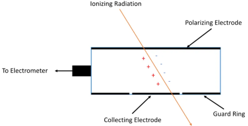
In this work, a plane-parallel plate ionization chamber is used, therefore the general composition of this type is described. Figure 3.1 is a simplified diagram of a plane-parallel plate ionization chamber. The cavity volume, which is filled with air, is bordered by the polarizing, collecting and guard electrodes. The polarizing electrode establishes the electric field in the air cavity since it is directly connected to the power supply. The collecting electrode is connected to the guard and has the function of collecting the produced charges, which is then measured by an electrometer. The electrometer must be capable of measuring very small output current which is of the order of femtoamperes to picoamperes, depending on the chamber design, radiation dose and applied voltage. The guard electrode, also called the guard ring, limits the sensitive volume of the chamber and avoids leakage current of the chamber to be collected by the collecting electrode [19, 33]. + + + + -To Electrometer Polarizing Electrode Guard Ring Ionizing Radiation Collecting Electrode

Figure 3.1: Schematic diagram of the composition of a plane-parallel plate ionization chamber.

According to the reciprocity theorem, if a small detector is used in a broad beam of a specific size or if a large sensitive area detector of a specific size is used with a small beam, the same results are obtained, if both source and detector are located in a homogeneous medium [16]. In spot scanning proton therapy systems, protons are delivered in very narrow beams (the so called pencil beams). Large detectors are thus often used for relative dosimetry measurements.

Ideally, these detectors would be used for dose reference measurements, however, PSDLs do not provide calibration coefficients (ND,w,Q0) for large area chambers. The latter are routinely used in the clinic for percent depth-dose and range measurements and small area chambers are typically used for dose reference measurements.

For an air-filled ionization chamber irradiated by a proton beam of quality Q, the average dose-to-air is given by: ¯

Dair,Q= MQ· (Wair/e)Q

⇢air· Vcavity (3.6)

where MQrepresents the measured charge in the cavity, ⇢air· Vcavityis the mass of air in the cavity and (Wair/e)Qis

the mean energy required to produce an ion pair in air.

Dose-to-water can be simply obtained with an ionization chamber by applying Bragg-Gray (or Spencer-Attix) cavity theory. Thus, dose-to-water, Dwater,Q, in a proton beam of quality Q is proportional to the average dose-to-air in

the air cavity volume, ¯Dair,Q, by:

Dwater,Q= ¯Dair,Q· (swater,air)Q· pQ (3.7)

where swater,airis the Bragg-Gray (or Spencer-Attix) mass collision stopping power ratio between water and air for the

charged particles spectrum at the measurement point in water and pQis the perturbation correction factor to account for

deviations from the conditions under which Bragg-Gray cavity theory is valid.

Replacing the extended form of the average dose-to-air in equation 3.6, an overall expression for dose-to-water is obtained: Dwater,Q=⇥MQ⇤· " 1 ⇢air· Vcavity #

·⇥(Wair/e)Q· (swater,air)Q· pQ⇤ (3.8)

It is important to highlight that the air cavity volume of commercial ionization chambers is not known accurately so it can be calculated through the following expression:

1 ⇢air· Vcavity

= ND,w,Q0

(Wair/e)Q0· (swater,air)Q0· pQ0

(3.9) where ND,w,Q0is the calibration coefficient of the dosimeter in terms of absorbed dose-to-water in the beam quality Q0, which is the reference beam quality, usually taken to be a Cobalt-60 beam. Note that all quantities in this equation refer to the beam quality Q0. By substituting equation 3.8 into the equation 3.7, dose-to-water can be expressed in the same

form as presented in the IAEA TRS-398 (section 1.3): Dwater,Q= MQ· ND,w,Q0·

(Wair/e)Q· (swater,air)Q· pQ

(Wair/e)Q0· (swater,air)Q0· pQ0

(3.10) with:

(Wair/e)Q· (swater,air)Q· pQ

(Wair/e)Q0· (swater,air)Q0· pQ0

= kQ,Q0 (3.11)