Valuation of barrier options through trinomial trees

I

S

C

T

E

D

F

U

L

F

D

M

V

ALUATION OF

B

ARRIER

O

PTIONS

THROUGH

T

RINOMIAL

T

REES

Gonçalo Nuno Henriques Mendes

Master in Financial Mathematics

2011

U

L

F

D

M

V

ALUATION OF

B

ARRIER

O

PTIONS

THROUGH

T

RINOMIAL

T

REES

Gonçalo Nuno Henriques Mendes

Master in Financial Mathematics

2011

I

S

C

T

E

D

F

I

Resumo

Os modelos das árvores (“lattice”) Binomial e Trinomial assumem que o processo estocástico do activo subjacente é discreto, isto é, o activo subjacente pode tomar um número finito de valores (cada um com uma determinada probabilidade associada) num pequeno intervalo de tempo.

A avaliação de opções com barreira usando métodos numéricos, nomeadamente os modelos Binomial/Trinomial, pode se tornar numa tarefa bastante delicada.

Enquanto o uso de um número elevado de “intervalos de tempo” pode produzir bons resultados para o caso das opções standard, o mesmo não se pode garantir para as opções com barreira, podendo mesmo produzir resultados errados. A origem deste problema surge da localização da barreira face aos nós da árvore adjacentes. Se a barreira se posicionar entre diferentes nós da árvore (e não tocar nos nós), os erros poderão ser muito significativos.

Ritchken [1995] sugere um algoritmo bastante eficiente, através do qual se constrói uma árvore cuja barreira intersecta os nós, permitindo assim resultados mais correctos. O objectivo desta dissertação é o de estudar o algoritmo proposto por Ritchken [1995].

Palavras-chave: Black-Scholes-Merton, Opções com Barreira, Arvores Trinomiais,

Ritchken

Abstract

The lattice methods, i.e. binomial and trinomial trees, assume that the underlying stochastic process is discrete, i.e. the underlying asset can change to a finite number of values (each associated with a certain probability) with a small advancement in time. Pricing barrier options using lattice techniques can be quite delicate.

While the use of a large number of time steps may produce accurate solutions for standard options, the use of the same number of time steps in valuing barrier options will often produce erroneous option values. The source of the problem arises from the location of barrier with respect to adjacent layers of nodes in the lattice. If the barrier falls between layers of the lattice, the errors may be quite significant.

Ritchken [1995] provides a highly efficient algorithm which produces a lattice where the nodes hit the barrier.

The purpose of this dissertation is to study the Ritchken [1995] algorithm.

Keywords: Black-Scholes-Merton, Barrier Options, Trinomial Trees, Ritchken JEL Classification: G12, G13

III

Acknowledgements

On concluding this endeavour, there are some people to whom I would like to express my gratitude;

Firstly, to Alexandra Ramada and Nélia Camera, when I was still working for MERCER. Their encouragement was greatly responsible for providing me with the necessary motivation to undertake this task.

Then, to Eduardo Dias and Filomena Santos from BES-VIDA, for all their support and understanding towards me and the responsibility of the task I had previously undertaken.

Also to my master’s colleagues and their huge contribution towards my success: Ângela Rocha, Lilia Alves and Marta Umbelino.

To my wife, Tânia. This thesis would not have been possible without her support and encouragement. This has became another one of our joint ventures and I’m very happy and proud of it.

Notation

– a point in ‘natural’ time; – Ending time (maturity);

– Value of the underlying asset at time t; – Exercise price (also known as “Strike”); – Barrier;

– Rebate;

– Risk-free interest rate; – Asset/dividend yield; – Volatility;

– Factor of an upward movement; – Factor of a downward movement;

– Probability of an upward movement; – Probability of a downward movement;

V

Table of Contents

1. Introduction ... 1

2. Binomial and Trinomial Models for Vanilla Options ... 2

2.1. Options ... 2

2.2. Black-Scholes-Merton Model ... 3

2.3. Binomial Model ... 7

2.4. Trinomial Model ... 13

3. Barrier Options under the Ritchken Trinomial Tree ... 16

3.1. Barrier Options ... 16 3.1.1. Down-and-in Call ... 17 3.1.2. Up-and-in Call ... 17 3.1.3. Down-and-in Put ... 17 3.1.4. Up-and-in Put ... 18 3.1.5. Down-and-out Call ... 18 3.1.6. Up-and-out Call ... 18 3.1.7. Down-and-out Put ... 19 3.1.8. Up-and-out Put ... 19 3.2. Relationships ... 20

3.3. Ritchken Trinomial Tree... 21

4. Implementation and Numerical Results ... 25

5. Conclusions ... 34

6. Appendix ... 35

6.1. “Black-Scholes-Merton” Pricing Formulas ... 35

6.1. Matlab Code ... 39

List of Figures and Tables

Figures:

Figure 1: Binomial Tree ... 7

Figure 2: Barrier assumed by binomial and trinomial tree lattices... 21

Figure 3: Down Barrier with and λ under Ritchken *1995+ ... 24

Figure 4: Trinomial Tree for a Down-and-Out call option ... 27

Figure 5: Trinomial Tree for a Down-and-Out call option under Ritchken [1995] ... 28

Tables:

Table 2: Convergence for Up-and-Out Options ... 30

Table 3: Down-and-Out Call - Sensitivities ... 31

1. Introduction

Derivatives with a more complicated payoff structure than simple vanilla options are called exotic options. Most exotic options are path dependent, meaning that their payoff is dependent on what path the underlying asset takes during the life of the option. Barrier options are path-dependent exotic derivatives whose value depends on the underlying having breached a given level, the barrier, during a certain period of time.

Ideally we would want to find closed form solutions for all exotic options. As the payoff structures of the exotic options become more complicated, so does the difficulty in finding closed form solutions. In most cases closed-form solutions do not exist, eg. American barrier options and these must be valued by using numerical methods.

The lattice methods, i.e. binomial and trinomial trees, assume that the underlying stochastic process is discrete, i.e. the underlying asset can change to a finite number of values (each associated with a certain probability) with a small advancement in time.

Pricing barrier options using lattice techniques can be quite delicate. While the use of a large number of time steps may produce accurate solutions for standard options, the use of the same number of time steps in valuing barrier options will often produce erroneous option values. The source of the problem arises from the location of barrier with respect to adjacent layers of nodes in the lattice. If the barrier falls between layers of the lattice, the errors may be quite significant. Ritchken [1995] provides a highly efficient algorithm which produces a lattice where the nodes hit the barrier.

The thesis is organized as follows. In Section 2, an introduction to standard options is made and both Binomial and Trinomial models for Vanilla Options are developed. Section 3 presents Barrier Options, and describes the method proposed by Ritchken [1995] to value them. Section 4 presents the algorithm and the main results obtained (it also includes the results provided on original paper). Finally, Section 5 concludes the thesis.

2.

Binomial and Trinomial Models for Vanilla

Options

2.1.

Options

An option is an agreement between two parties, the option seller and the option buyer, whereby the option buyer is granted a right (but not an obligation), secured by the option seller, to carry out some operation (or exercise the option) at some moment in the future. The predetermined price is referred to as strike price, and future date is called expiration date.

Options come in two varieties: A call option grants its holder the right to buy the underlying asset at a strike price at some moment in the future. A put option gives its holder the right to sell the underlying asset at a strike price at some moment in the future.

There are several types of options, mostly depending on when the option can be exercised. European options can be exercised only on the expiration date. American-style options are more flexible as they may be exercised at any time up to and including expiration date and as such, they are generally priced at least as high as corresponding European options. Other types of options are path-dependent or have multiple exercise dates (Asian, Bermudian).

For a call option, the profit made at the exercise date is the difference between the price of the asset on that date and the strike price, minus the option price paid. For a put option, the profit made at exercise date is the difference between the strike price and the price of the asset on that date, minus the option price paid.

The call option terminal payoff is defined mathematically as

1. where is the asset price at expiration date and is the exercise price. Similarly, the terminal payoff of the put option is defined as

2.2.

Black-Scholes-Merton Model

The Black-Scholes-Merton model develops on the assumption that an asset price follows a geometric Brownian motion with constant drift and volatility, a continuous-time, continuous-variable stochastic process also called a generalized Wiener process that satisfies, under the equivalent martingale measure that takes the “money-market account” as numeraire, the equation

3. where is the asset price, is the continuously compounded risk-free interest rate, is the continuously compounded asset yield, is the standard deviation of the assets’ return or annualized volatility and is a Wiener process. By definition, follows a normal distribution with mean zero and variance rate equal to the time instant .

Using Itô's lemma1, and for any continuously differentiable function ,

4. One possible choice for could be . So the Itô’s process defined by is

5.

1 _{Itô's lemma: Let}

be an Itô process and a twice continuously

differentiable function in . On that conditions, the stochastic process defined by is an Itô process, and

where

Therefore, the change in between time zero and some future time is normally distributed, i.e.

6. where is a normal distribution with mean and variance .

Integrating both sides of equation (5.) between and we have that

7. Knowing that follows a normal distribution, the price of an asset at future time given its price today follows a log-normal distribution. The only source of uncertainty is the Wiener process which is the same for both and .

Let’s now consider a portfolio composed by the quantity Δ of the asset and by a short position in the derivative , the portfolio’s value is given by

8. We can now apply the Itô’s lemma to the portfolio’s value function

9. Using the definition of we have

10. Considering 11.

we now eliminate the stochastic component (relative to ) and the equation becomes simpler:

12. Therefore, the portfolio must be riskless for the period of time and, according to risk neutral valuation, must earn the same as other short-term risk-free securities or an arbitrage opportunity would arise. Hence,

13. When we substitute equations (8.), (11.) and (12.) into equation (13.) we obtain the Black-Scholes-Merton partial differential equation

14. This equation has many solutions corresponding to the different derivatives that can be defined on S. If we define the following boundary conditions

15. and solve the Black-Scholes-Merton partial differential equation we arrive at the following formula for the time zero price of an European option:

_16. where 17. 18.

and is the cumulative probability distribution function of the standard normal distribution.

From the put-call parity given by

_19.

we obtain the pricing formula for an European put option:

_20.

The following assumptions apart from the geometric Brownian motion were made while deriving the pricing formulas for European call and put options:

• It is possible to short-sell the asset with full use of the proceeds; • There are no transaction costs or taxes;

• Securities are perfectly divisible and trading is continuous; • There are no riskless arbitrage opportunities;

• The risk-free interest rate is constant for all maturities and one can borrow and lend at this rate.

2.3.

Binomial Model

The binomial option pricing model is an iterative solution that models the price evolution over the whole option validity period. For some types of options, such as the American options, using an iterative model is the only choice since there is no known closed-form solution that predicts the exact price over time.

Cox, Ross, and Rubinstein [1979] introduced the Binomial Model for pricing American stock options. This model is categorized as a Lattice Model or Tree Model because of the graphical representation of the stock price and option price over the large number of intervals or steps, during the time period from valuation to expiration, which are used in computing the option price.

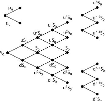
At each step, the price can only move up and down at fixed rates and with pseudo-probabilities and respectively. In other words, the root node is today’s price, each column of the tree represents all the possible prices at a given time, and each node of value as two child nodes of values and , where and are the factors of upward and downward movements for a single time-step .

The movements and are derived from volatility , where ; _.

The graphical representation of the model starts at the left with the stock price on the valuation date . At the first interval, the stock price can either branch up or down a calculated amount. From each of these two points the stock price can either branch up or down at the second interval, forming a lattice look. The branches continue, making a larger structure throughout the time intervals up to expiration date.

At expiration, the option values at each node are equal to the intrinsic value at that point, since the option is expired and has no time value at that point. The intrinsic values are then multiplied by their respective probabilities.

The model must then work backwards through each node, calculating the option value at each point. When it gets back to the left hand apex of the lattice, it has determined the present value of the option on the valuation date, using the risk-free interest rate. The total of the present values of all the individual potential paths is the option’s fair value.

Let’s see an illustration for a European Call Option (for which the expiration date is just one period away):

Let be the initial stock price (on the valuation date), which, at the end of the period can be valued as with probability or with probability .

We also assume that the interest rate is constant, individuals may borrow or lend as much as they wish at this rate; there are no transaction costs, or margin requirements and the individuals are allowed to sell short any security.

Letting denote the riskless interest rate over one period, we require . If these inequalities did not hold, there would be profitable riskless

arbitrage opportunities involving only the stock and riskless borrowing and lending.

Let be the current value of the call, and e the corresponding value at the end of the period if the stock price goes to or , respectively.

Therefore,

Assume we form a hedging portfolio containing shares of stock and the amount in riskless bonds, such that, at the end-of-period the values of the portfolio and the call for each possible outcome are the same. This will cost now, and at the end of the period, the value of this portfolio will be

It is also required that

21. Solving these equations, we have

22. Equation (21.) can also be rewritten as

23. If there are to be no riskless arbitrage opportunities, the current value of the Call and the hedging portfolio should be the same. Therefore, it must be true that

24. Equation (24.) can be simplified by defining

so that we can write

Note that, the probability is the value would have in equilibrium if investors were risk-neutral.

The expected rate of return on the stock would then be the riskless interest rate, so

and Hence, the call’s value can be interpreted as the expectation of its discounted future value in a risk-neutral world.

However, the market is not open for trading once a day, but instead trading takes place almost continuously.

Let’s now consider that , the time to expiration (maturity) is divided into number of periods with length , .

As trading takes place more and more frequently, gets closer and closer to zero. We must then adjust the interval-dependent variables , , and in such a way that we obtain empirically realistic results as becomes smaller, or, equivalently, as .

Consider the continuously compounded rate of return on the stock over each period (which is a random variable),

As an example, consider a sequence of five moves, say . Then the final stock price will be ; , and . More generally, over periods,

25. where is the (random) number of upward moves occurring during the periods to expiration.

Therefore, the expected value of is

26. and its variance is

27. Since the number of upward moves from periods follows a binomial distribution, . It is well known that

and

29. Combining , we have

30. 31. Since T is a fixed length of time, in searching for a realistic result, we must make the appropriate adjustments in , , and . Doing that, we would at least want the mean and variance of the continuously compounded rate of return of the assumed stock price movement to coincide with that of the actual stock price as . Suppose we label the actual empirical values of and as and

, respectively. Then we would want to choose , , and , so that

32. Imposing the restriction (the tree will recombine), and with a little algebra we can accomplish this by letting

33.

In this case, for any , and .

Clearly, as , while for all values of .

It is also shown on Cox, Ross, Rubinstein [1979], that the multiplicative binomial probability distribution of stock prices goes to the lognormal distribution.

Also, the resulting formulas are the same as those advanced by Black and Scholes [1973] and Merton [1973, 1977], since they began directly with continuous trading and the assumption of a lognormal distribution for stock prices as the method explained above.

2.4.

Trinomial Model

This model improves upon the Binomial Model by allowing a stock price to move up, down or stay the same with certain probabilities.

Trinomial trees provide an effective method of numerical calculation of option prices within the Black-Scholes equity pricing model. Trinomial trees can be built in a similar way to the binomial tree. To create the jump sizes and and the transition probabilities and in a binomial model we aim to match these parameters to the first two moments of the distribution of our geometric Brownian motion. The same can be done for our trinomial tree for ; ; ; ;

.

Let’s consider a trinomial tree model defined by 34. Thus, 35. 36. where we have used

In a risk neutral world with continuous time, the mean gross return is , where is the riskfree rate. So with equation (35.),

Thus we have an equation that links our first target moment, the mean return, with the four parameters ; ; ; .

In the Black–Scholes–Merton model we have lognormally distributed stock prices with variance

_38.

Dividing by and equating to Equation (36.), we obtain

_39.

which links our second target moment, , with our four parameters.

Conditions (37.) and (39.) impose two constraints on 4 parameters of the tree. An extra constraint comes from the requirement that the size of the upward jump is the reciprocal of the size of the downward jump,

40. This condition is not always used for a trinomial tree construction, however, it greatly simplifies the complexity of the numerical scheme, since it leads to a recombining tree, which has the number of nodes growing polynomially with the number of levels, rather than exponentially.

Given the knowledge of jump sizes ; and the transition probabilities , it is now possible to find the value of the underlying asset, , for any sequence of price movements.

Let us define the number of up, down and middle jumps as ; ; , respectively, and so the value of the underlying share price at node for time is given by

41.

We have imposed three constraints ((37.), (39.), (40.)) on four parameters ; ; and . So, there will be a family of trinomial tree models.

We’ll just consider the following popular representative of the family: its jump sizes are ; .

Its transition probabilities are then given by

42. 43. 44.

3. Barrier Options under the Ritchken

Trinomial Tree

3.1.

Barrier Options

Barrier options are path-dependent exotic derivatives whose value depends on the underlying having breached a given level, the barrier, during a certain period of time. The market for barrier options has grown strongly because they are cheaper then corresponding standard options and provide a tool for risk managers to better express their market views without paying for outcomes that they may find unlikely.

These types of options are either initiated or terminated upon reaching a certain barrier level; that is, they are either knocked in or knocked out.

A European knock-in option is an option whose holder is entitled to receive a standard European option if a given level is breached before expiration date or a rebate otherwise. A European knock-out option is a standard European option that ceases to exist if the barrier is touched, giving its holder the right to receive a rebate. In both cases the rebate can be zero.

The way in which the barrier is breached is important in the pricing of barrier options and, therefore, we can define down-and-in, up-and-in, down-and-out and up-and-out options for both calls and puts, giving us a total of eight different barrier options. There are more complex types of barrier options like double barrier options but we will not cover them in this text.

Also, these options could have rebates, which are pre-defined payouts which are sometimes given when a barrier option expires without being exercised. For this thesis purposes we won’t consider rebates because the barriers with rebates are not traded as much as barriers without.

3.1.1.

Down-and-in Call

The down-and-in call option gives its holder the right to receive a vanilla call option if the barrier H is hit or a rebate R otherwise. At inception the underlying price S is higher than the barrier H and has to move down before the regular option becomes active.

Expressed mathematically, the terminal payoff function is

45.

3.1.2.

Up-and-in Call

Like the down-and-in, the up-and-in call option gives its holder the right to receive a regular call option if the barrier H is breached or a rebate R otherwise, but the underlying price S starts below the barrier H and has to move up for the regular option to be activated.

The terminal payoff function is defined as

46.

3.1.3.

Down-and-in Put

A down-and-in put option gives its holder the right to receive a standard put option if the barrier H is hit or a rebate R otherwise. The underlying price S starts above the barrier H and has to move down before the vanilla put is born.

The terminal payoff function is expressed mathematically by

3.1.4.

Up-and-in Put

The up-and-in put option gives its holder the right to receive a regular put option if the barrier H is hit or a rebate R otherwise. At inception the underlying price S is lower than the barrier H and has to move up for the regular put option to become activated.

Expressed mathematically, the terminal payoff function is

48.

3.1.5.

Down-and-out Call

A down-and-out call option is a regular call option that expires worthless or pays rebate R as soon as the barrier H is hit. At inception the underlying price S is higher than the barrier H.

The terminal payoff function is expressed as

49.

3.1.6.

Up-and-out Call

The up-and-out call option is a regular call option that expires and pays rebate R if the barrier H, above the underlying price S at inception, is breached.

Expressed mathematically, the terminal payoff function is

3.1.7.

Down-and-out Put

A down-and-out put option is a regular put option while the barrier H is not hit. If the barrier is breached, then a rebate R is paid. In the beginning the underlying price S is higher than the barrier.

The terminal payoff function is given by

51.

3.1.8.

Up-and-out Put

The up-and-out put option is a vanilla put option that expires paying a rebate R as soon as the barrier H, above the underlying price S at inception, is hit.

Expressed mathematically, the terminal payoff function is

3.2.

Relationships

Considering that there is no any rebate, we can obtain some relationships between vanilla and barrier options.

Suppose that we have a portfolio composed by a and-in call and a down-and-out call with identical characteristics and no rebate.

If the barrier is never hit the down-and-out call provides us a standard call, otherwise, the down-and-out call expires worthless but the down-and-in call emerges as a standard call.

Either way we end up with a vanilla call so the following relationship between barrier options and vanilla options must hold when the rebate is zero:

53. With a similar reasoning we can reach the same relationships for the other barrier options

54. 55. 56.

3.3.

Ritchken Trinomial Tree

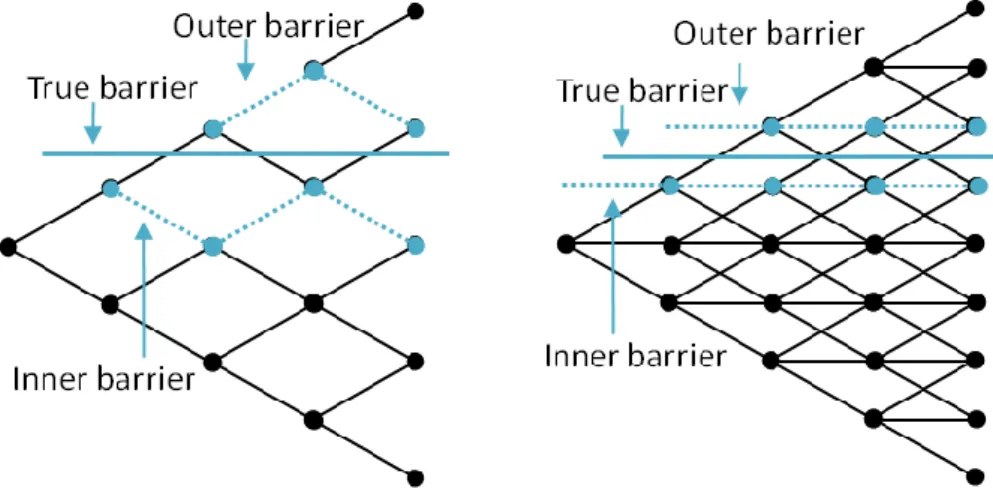
Barrier options can be priced by lattice techniques such as binomial or trinomial trees. However, even in continuously monitored barrier options, the convergence of the lattice approach is very slow and requires a quite large number of time steps to obtain a reasonably accurate result. This happens because the barrier being assumed by the tree is different from the true barrier.

Define the inner barrier as the barrier formed by nodes just on the inside of the true barrier and the outer barrier as the barrier formed by nodes just outside the true barrier. Figure below shows the inner and outer barrier for a binomial and trinomial tree when the true barrier is horizontal and constantly monitored. The usual tree calculations implicitly assume the outer barrier is the true barrier because the barrier condition is first met on the outer barrier.

Figure 2:Barrier assumed by binomial and trinomial tree lattices

Ritchken [1995] provided an effective method to deal with this situation, since he describes a method where the nodes always hit the barrier.

Here we briefly review the trinomial lattice implementation provided by Kamrad and Ritchken [1991] and Ritchken [1995].

It is well-known that trinomial and higher order multinomial lattice procedures can be used as an alternative to the binomial lattice.

Assume the underlying asset follows a Geometric Wiener Process which, for valuation purposes has drift , where is the riskless rate, is the dividend yield and is the instantaneous volatility. Then

57. where is a normal random variable whose first two non-central moments are equal to and , respectively.

Let be the approximating distribution for over the period . is a discrete random variable with the following distribution

58. where .

The first two non-central moments of the approximating distribution are chosen to be the same as the ones from . Specifically we have:

59. 60. Solving these equations, we have:

61.

And finally, as then

62. Thus, for a sufficiently small , the transition probabilities are given by

63. 64. 65. can be viewed as a parameter that controls the gap between layers of prices on the lattice, and is referred to as the “stretch parameter”.

Notice that if then , and the expressions collapse to the binomial model of Cox, Ross and Rubinstein [1979].

The advantage of this trinomial representation is that the extra parameter allows us to decouple the time partition from the state partition. For ordinary options, Kamrad and Ritchken [1991] show that selecting such that the horizontal jump probability is one third produces very rapid convergence in prices, and is computationally more efficient than a binomial lattice with twice as many time partitions.

To price barrier options, Ritchken [1995] provides a procedure to determine the stretch parameter such that the barrier is hit exactly.

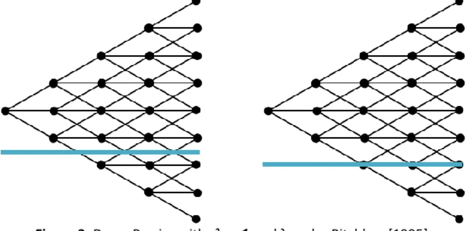
To make the explanation clear, consider the down-an-out call option where represents the knock-out barrier.

Starting with , we compute the number of down moves that leads to the lowest layer of nodes above the barrier, H. This value, , say, is the largest integer smaller than , where is defined by

66. If is an integer, then we shall maintain , otherwise we should consider such that .

By other words, it’s the same as compute (as defined on equation (66.)) and consider Then if we should keep , otherwise we should consider .

Under this construction . With this specifications of , the trinomial approximation will result in a lattice that will produce a layer of nodes that coincides with the barrier.

Bellow two figures are shown that illustrate a down barrier option when , i.e. when the nodes do not hit the barrier, and with under Ritchken [1995], where the nodes hit the barrier.

4. Implementation and Numerical Results

Here we briefly describe the algorithms used to set up the valuation for Knock-Out options (calls and puts for both Down-and-Knock-Out and Up-and-Knock-Out options), as well for European and American style options.

We left the algorithm for knock-in as a future improvement on this thesis. However, if there is no rebate we can use de relationships provided on Section 3.2 to get the values for the European style knock-in options.

ALGORITHM:EUROPEAN KNOCK-OUT BARRIER OPTIONS UNDER RITCHKEN [1995]  Find lambda according to Ritchken [1995]:

o Compute

o Compute , if then keep , else set .

 Calculate the jump sizes , and ;

 Calculate the transition probabilities , and ;

 Build the share price tree:

 Calculate the payoff of the option at maturity, :

o DO call: o DO put: o UO call: o UO put:

 Calculate option price at node (backward induction)

for do o DO: o UO: Otherwise end for

ALGORITHM:AMERICAN KNOCK-OUT BARRIER OPTIONS UNDER RITCHKEN [1995]  Find lambda according to Ritchken [1995]:

o Compute

o Compute , if then keep , else set .

 Calculate the jump sizes , and ;

 Calculate the transition probabilities , and ;

 Build the share price tree:

 Calculate the payoff of the option at maturity, :

o DO call: o DO put: o UO call: o UO put:

 Calculate option price at node (backward induction)

for do o Call option: or o Put option: or Otherwise end for

Output option price

Case 1:

Consider a Down-and-Out Call option with the same parameters as was done on Ritchken [1995] paper:

; ;

- Scenario (i): , which is the same as using the Binomial Tree (as explained before).

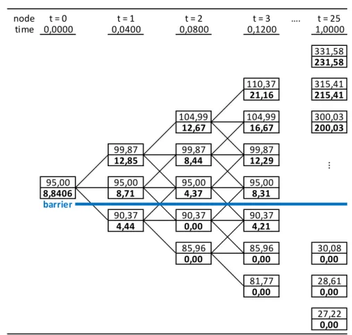
- Scenario (ii): with “stretch” parameter from Ritchken *1995+; For the first scenario, we have

;

; ;

Figure 4: Trinomial Tree for a Down-and-Out call option At each node (trees) we have:

Upper Value = Underlying Asset Price Lower Value = Option Price

node t = 0 t = 1 t = 2 t = 3 …. t = 25 time 0,0000 0,0400 0,0800 0,1200 1,0000 331,58 231,58 110,37 315,41 21,16 215,41 104,99 104,99 300,03 12,67 16,67 200,03 99,87 99,87 99,87 12,85 8,44 12,29 95,00 95,00 95,00 95,00 8,8406 8,71 4,37 8,31 barrier 90,37 90,37 90,37 4,44 0,00 4,21 85,96 85,96 30,08 0,00 0,00 0,00 81,77 28,61 0,00 0,00 27,22 0,00 ⋮

Thus, we obtain an option value of 8,8406 for this Down-and-Out call, as shown on figure 4. We can easily notice that, as supposed, the barrier does not hit the tree nodes.

A different thing happens on the second scenario, where we consider the stretch parameter from Ritchken [1995].

For the second scenario, we have

;

; ;

Figure 5: Trinomial Tree for a Down-and-Out call option under Ritchken [1995]

node t = 0 t = 1 t = 2 t = 3 …. t = 25 time 0,0000 0,0400 0,0800 0,1200 1,0000 367,07 267,07 111,73 347,75 21,78 247,75 105,85 105,85 329,45 11,23 16,32 229,45 100,28 100,28 100,28 11,43 5,79 11,02 95,00 95,00 95,00 95,00 6,0069 5,90 0,00 5,68 barrier 90,00 90,00 90,00 0,00 0,00 0,00 85,26 85,26 27,39 0,00 0,00 0,00 80,78 25,95 0,00 0,00 24,59 0,00 ⋮

In this case the option price is 6,0069 which is close to the accurate value provided by Black-Scholes formulas, 5,9968.

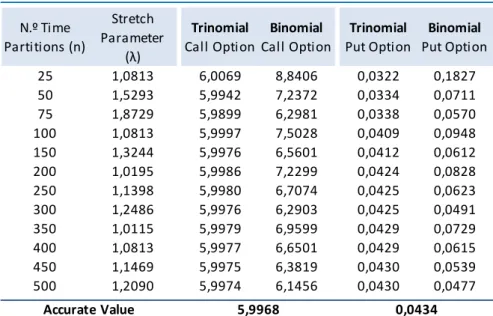
The table below shows the convergence values for this DO call option using the two scenarios above, as well for the put with same parameters. For each time partition, the value of the stretch parameter is reported.

Table 1: Convergence for Down-and-Out Options

We easily observe the very rapid convergence for the down-and-out prices. Table 2 shows the results obtained for the other knock-out options: Up-and-Out call and put options. These options have the same parameters as the previous Down-and-Out options, with the exception of barrier level, which for this case is 110 (obviously above the strike).

N.º Time Partitions (n) Stretch Parameter (λ) Trinomial Call Option Binomial Call Option Trinomial Put Option Binomial Put Option 25 1,0813 6,0069 8,8406 0,0322 0,1827 50 1,5293 5,9942 7,2372 0,0334 0,0711 75 1,8729 5,9899 6,2981 0,0338 0,0570 100 1,0813 5,9997 7,5028 0,0409 0,0948 150 1,3244 5,9976 6,5601 0,0412 0,0612 200 1,0195 5,9986 7,2299 0,0424 0,0828 250 1,1398 5,9980 6,7074 0,0425 0,0623 300 1,2486 5,9976 6,2903 0,0425 0,0491 350 1,0115 5,9979 6,9599 0,0429 0,0729 400 1,0813 5,9977 6,6501 0,0429 0,0615 450 1,1469 5,9975 6,3819 0,0430 0,0539 500 1,2090 5,9974 6,1456 0,0430 0,0477 Down-and-Out Option Accurate Value 5,9968 0,0434

Table 2: Convergence for Up-and-Out Options

For these up-and-out options, we observe that the trinomial results provided do not converge for the accurate value: sometimes the figures are close to the accurate value, but it depends on the number of time-steps considered.

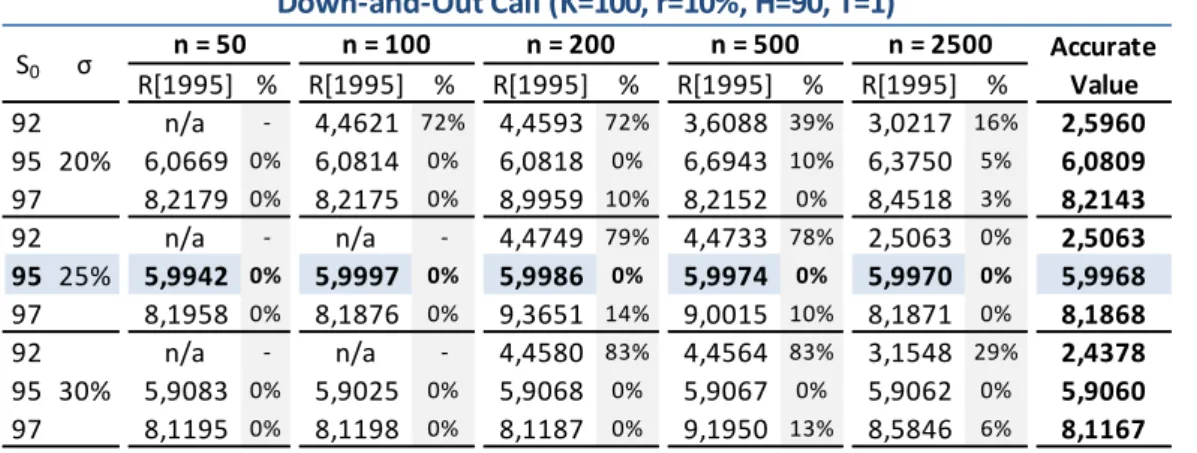
Let’s now consider some stress on initial stock prices and volatility , for the same Down-and-Out call mentioned before. Table 3 illustrate the values obtained, considering the scenarios with and , the results in the middle (blue) are the original ones and .

For each number of time-steps , Table 3 shows the value obtained and the error (%) with respect to the accurate value reported (column at the end).

N.º Time Partitions (n) Stretch Parameter (λ) Trinomial Call Option Binomial Call Option Trinomial Put Option Binomial Put Option 25 1,4660 0,5532 0,0000 6,7117 5,7234 50 1,0366 0,0826 0,2534 5,6957 6,2322 75 1,0157 0,2156 0,2262 6,2105 6,1768 100 1,1728 0,2163 0,0756 6,2087 5,7513 150 1,0260 0,1735 0,1438 6,0789 6,0077 200 1,0366 0,0867 0,1426 5,6913 5,9357 250 1,0302 0,1507 0,1272 5,9988 5,9168 300 1,0157 0,0879 0,1373 5,6916 5,9267 350 1,0971 0,0880 0,0902 5,6915 5,6975 400 1,0662 0,1382 0,0945 5,9468 5,7579 450 1,0366 0,0879 0,1131 5,6909 5,8221 500 1,0087 0,1302 0,1224 5,9103 5,8856 Up-and-Out Option Accurate Value 0,0889 5,6907

Table 3: Down-and-Out Call - Sensitivities

We easily observe that it is extremely difficult to achieve convergence when the barrier is close to the current price of the underlying asset (the “near-barrier” problem), or when we increase the volatility.

R[1995] % R[1995] % R[1995] % R[1995] % R[1995] % 92 n/a - _4,4621 72% _4,4593 72% _3,6088 39% _3,0217 16% _2,5960 95 20% 6,0669 0% 6,0814 0% 6,0818 0% 6,6943 10% 6,3750 5% 6,0809 97 8,2179 0% 8,2175 0% 8,9959 10% 8,2152 0% 8,4518 3% 8,2143 92 n/a - n/a - 4,4749 79% 4,4733 78% 2,5063 0% 2,5063 95 25% 5,9942 0% 5,9997 0% 5,9986 0% 5,9974 0% 5,9970 0% 5,9968 97 8,1958 0% _8,1876 0% _9,3651 14% _9,0015 10% _8,1871 0% _8,1868 92 n/a - _n/a - _4,4580 83% _4,4564 83% _3,1548 29% _2,4378 95 30% 5,9083 0% _5,9025 0% _5,9068 0% _5,9067 0% _5,9062 0% _5,9060 97 8,1195 0% _8,1198 0% _8,1187 0% _9,1950 13% _8,5846 6% _8,1167 Down-and-Out Call (K=100, r=10%, H=90, T=1) Accurate Value n = 50 n = 100 n = 200 n = 500 σ S0 n = 2500

Case 2:

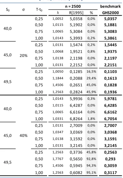
Consider the following set of twenty-four contracts, American-Style Up-and-Out

Put options, that have different values of the underlying asset price at valuation date , of the time-to-expiration , and of the volatility parameter .

The barrier level and the strike value are fixed at and , respectively. The risk-free rate is chosen to be .

We choose , , and . As a result, the set of contracts include out-of-the-money, at-the-money, and in-the-money options.

Table 4 summarizes the option prices for the trinomial Ritchken [1995] method, with twenty-five hundred time steps, in relation to the benchmark used on Gao-Huang-Subramahnyam [2000] (the Ritchken (1995) method with at least ten thousand time-steps).

We also observe that it is particularly hard to achieve convergence when the barrier is close to the current price of the underlying asset, or when we increase the volatility.

Table 4: American-Style Up-and-Out Put

Gao-Huang-Subramahnyam [2000] develop one method that is free of the difficulty in dealing with spot prices in the proximity of the barrier, the case where the barrier options are most problematic. However, the implementation of such quasi-analytical pricing method is outside the scope of the present dissertation.

benchmark λ R[1995] % GHS2000 0,25 1,0052 _5,0358 0,0% _5,0357 0,50 1,0115 _5,1902 0,0% _5,1881 0,75 1,0065 5,3084 0,0% 5,3083 1,00 1,0143 _5,3993 0,2% _5,3861 0,25 1,0131 1,5474 0,2% 1,5445 0,50 1,0068 _1,9521 0,8% _1,9375 0,75 1,0138 2,1198 0,0% 2,1197 1,00 1,0131 _2,2152 0,0% _2,2151 0,25 1,0050 0,1285 16,5% 0,1103 0,50 1,1844 _0,2088 29,4% _0,1613 0,75 1,4506 0,2651 45,0% 0,1828 1,00 1,2563 0,2824 45,9% 0,1936 0,25 1,0143 _5,9936 0,3% _5,9781 0,50 1,0115 6,4287 0,0% 6,4285 0,75 1,0065 _6,6164 0,0% _6,6162 1,00 1,0331 6,8264 1,8% 6,7054 0,25 1,0131 _2,7009 0,0% _2,7007 0,50 1,0347 3,0369 0,0% 3,0368 0,75 1,0138 _3,1592 0,0% _3,1591 1,00 1,0131 3,2145 0,0% 3,2145 0,25 1,2563 _0,3736 45,8% _0,2563 0,50 1,7767 0,5650 92,8% 0,293 0,75 1,4506 _0,5945 94,3% _0,3059 1,00 1,2563 0,6082 95,1% 0,3117 American Style Up-and-Out Put

(K=45, r=4.88%, H=50) n = 2500 20% 40% T-t0 40,0 45,0 49,5 S0 σ 49,5 45,0 40,0

5. Conclusions

It has been recognized that the simple binomial method is not appropriate for pricing barrier options due to the fact that the price of such options is very sensitive to the location of the barrier in the lattice.

This research project addressed the problems involved in pricing barrier options using lattice techniques. If simple binomial models are used, large errors may result.

The source of the problem arises from the location of the barrier with respect to adjacent layers of nodes in the lattice; usually the barrier does not coincide with a layer of nodes, which may produce erroneous results.

The main focus of the project was the implementation of Ritchken [1995] which provides an effective method to deal with this situation; he describes a method where the nodes always hit the barrier, so the barrier being assumed by the tree is the true one.

The problem with these approaches is that as the asset price gets close to the barrier, the number of time steps needed to value this option goes to infinity. As a suggestion, for those cases one could use the method proposed by Gao-Huang-Subramahnyam [2000].

6. Appendix

6.1.

“Black-Scholes-Merton” Pricing Formulas

Merton (1973) and Rubinstein (1991a) derived the following closed formulas for the pricing of European barrier options.

_{67. 68. 69. 70. 71.} 72. 73. 74. 75. 76. 77. 78. where .

































6.1.

Matlab Code

The following Matlab code is the main function used to get all the results posted on this thesis. function [n,lambda,price] = TrinomialBarrierOptions(BO,CP,EA,Tree,S0,K,sigma,t,T,rf,H,n,R) % INPUT VARIABLES %

% BO: "Barrier Option":

% 'DO' - DOWN-and-OUT barrier option % 'UO' - UP-and-OUT barrier option %

% CP: 'C' - CALL option % 'P' - PUT option %

% EA: 'E' - European Style option % 'A' - American Style option %

% TREE: 'T' - TRINOMIAL tree, otherwise uses BINOMIAL %

% S0: Spot (@Start Date) % K: Strike

% sigma: Volatility % t: Start Date % T: Maturity

% rf: risk free rate % H: Barrier

% T: Maturity

% n: number of time partitions % R: Rebate

dt = (T-t)/n;

if (Tree == 'T') %Trinomial figures

%find lambda to use on Trinomial tree for Barrier Options

eta = log(S0/H)/(sigma*sqrt(dt)); n0 = fix(eta);

if(eta == n0) %eta is an integer

lambda=1; else

lambda = eta/n0; end

else

lambda=1; %uses Binomial tree

end

u = exp(lambda*sigma*sqrt(dt)); %m = 1; not necessary in this code

%d = 1/u; not necessary in this code

niu = rf - 0.5*(sigma^2); %drift

%transition probabilities

pu = 1/(2*lambda^2) + niu*sqrt(dt)/(2*lambda*sigma); pm = 1 - 1/lambda^2;

pd = 1/(2*lambda^2) - niu*sqrt(dt)/(2*lambda*sigma);

%set auxiliar number of rows (matrix) n_lin = 2*n+1;

%compute the stock price at each node for j=1:n+1 for i=n-j+2:n+j S(i,j)=S0*u^(n-i+1); end end

%compute payoff at maturity switch BO case {'DO'} for i=1:n_lin if(S(i,n+1)<=H) P(i,n+1) = R; else if(CP =='C') P(i,n+1) = max(S(i,n+1)-K,0); else P(i,n+1) = max(K-S(i,n+1),0); end end end case {'UO'} for i=1:n_lin if(S(i,n+1)>H) P(i,n+1) = R; else if(CP =='C') P(i,n+1) = max(S(i,n+1)-K,0); else P(i,n+1) = max(K-S(i,n+1),0); end end end end

%compute payoffs at all other time steps switch BO

case {'DO'} j=n; while j>0

if(S(i,j)>H) if (EA == 'E') P(i,j)=exp(-rf*dt)*(pu*P(i-1,j+1)+pm*P(i,j+1) +pd*P(i+1,j+1)); else if(CP =='C') P(i,j)=max(exp(-rf*dt)*(pu*P(i-1,j+1)+pm*P(i,j+1) +pd*P(i+1,j+1)),S(i,j)-K); else P(i,j)=max(K-S(i,j),exp(-rf*dt)*(pu*P(i-1,j+1) +pm*P(i,j+1)+pd*P(i+1,j+1))); end end else P(i,j) = 0; end end j=j-1; end case {'UO'} j=n; while j>0 for i=n-j+2:n+j if(S(i,j)<=H) if (EA == 'E') P(i,j)=exp(-rf*dt)*(pu*P(i-1,j+1)+pm*P(i,j+1) +pd*P(i+1,j+1)); else if(CP =='C') P(i,j) = max(exp(-rf*dt)*(pu*P(i-1,j+1)+pm*P(i,j+1) +pd*P(i+1,j+1)),S(i,j)-K); else P(i,j) = max(K-S(i,j),exp(-rf*dt)*(pu*P(i-1,j+1) +pm*P(i,j+1)+pd*P(i+1,j+1))); end end else P(i,j) = 0; end end j=j-1; end end price = P(n+1,1);

7. Bibliography

 BLACK, F. and M. SCHOLES, 1973, “The Pricing of Options and Corporate

Liabilities”, Journal of Political Economy 81, 637-654.

 COX, J., S. ROSS and M. RUBINSTEIN, 1979, “Option Pricing, A Simplified

Approach”, Journal Financial Economics 7, 229-263.

 GAO,B.,HUANG J. AND M.SUBRAMAHNYAM, 2000, “The Valuation of American

Barrier Options Using the Decomposition Technique”, Journal of

Economics Dynamics & Control, 24, 1783-1827.

 GILLI,M. and E. SCHUMAN, 2009, “Implementing Binomial Trees”, COMISEF WPS 8.

 HULL J.,2000, “Options, Futures and Other Derivative Securities”, Fourth Edition, Prentice–Hall.

 RITCHKEN,P. and B. KAMRAD, 1991, “Multinomial Approximating Models for

Options with k State Variables”, Management Science, Volume 37, Issue

12, 1640-1652.

 RITCHKEN, P., 1995, “On Pricing Barrier Options”, The Journal of