Was there a structural change, after 2009, in the
relation between macroeconomic and the stock
market’s performance in the United States?
Pedro Melo, 152217008
Dissertation written under the supervision of
Professor João Valle e Azevedo
.
Dissertation submitted in partial fulfilment of requirements for the MSc in
Economics, at the Universidade Católica Portuguesa, 24
thof February 2020.
2
Was there a structural change, after 2009, in the relation between
macroeconomic and the stock market’s performance in the United States?
by Pedro Melo
Abstract
During the lasts 10 years, stock markets have witnessed consecutive historical maxima, namely the S&P500 index. Parallelly, the associated Cyclically-Adjusted Price-to-Earnings ratio (CAPE) followed the same path, being substantially above the historic average. In the same line, Cochrane (2011) excess returns regression seems to suggest overvalued stock prices, similar to the periods that ended at the Dotcom bubble and the Great Recession. Moreover, looking 5 years ahead it seems to suggest a stable forecasted path what can mean a correction of the actuals’ excess returns over the next years.
In order to get some clues about this bull-market, this dissertation focuses on the relation between macroeconomic and stock market performance proxied by the S&P500 index from 2009 to 2019. In particular, investigates the relations between the stock market and the economic activity, monetary policy and the companies’ financial performance (of the companies that integrate the index), through two Structural Vector Auto-Regression (SVAR), resorting to the Cholesky decomposition. We find that, comparing with the two previous post-recessions periods, the current one appears to have a higher positive sensitivity of the stock market to a shock on the economic activity and on the financial performance of companies (better conditions), as well as a significant negative short-term reaction to a shock on monetary policy (tightening). This relation with the monetary policy is strengthened by our LOGIT model that approaches the significant relation of the US Federal Reserves’ monetary policy surprise announcements on the S&P500 index stock returns.
Keywords: S&P500 equity index bull market, unconventional monetary policy, economic activity impact.
3
Was there a structural change, after 2009, in the relation between
macroeconomic and the stock market’s performance in the United States?
by Pedro Melo
Resumo
Os últimos 10 anos foram marcados por consecutivos máximos históricos nos mercados acionistas, nomeadamente no índice S&P500. Paralelamente, o rácio associado “Cyclically-Adjusted Price-to-Earnings” (CAPE) acompanhou a mesma tendência tendo registado valores acima da média histórica.
Da mesma maneira, segundo a regressão dos “excess returns” apresentada por Cochrane (2011), é possível evidenciar valores sobrevalorizados, um comportamento similar aos períodos que terminaram na bolha Dotcom e na Grande Recessão. Ademais, olhando para um horizonte de 5 anos, constata-se uma trajetória estável dos retornos previstos o que poderá evidenciar uma correção dos atuais ao longo dos próximos anos.
De forma a obter algumas pistas sobre o “bull market”, esta tese foca a relação entre a performance macroeconómica e a do mercado acionista, recorrendo ao índice S&P500 como
proxy, de 2009 a 2019. Por outras palavras, investiga as relações entre o mercado acionista e
atividade económica, política monetária, e a performance financeira das empresas que compõem o índice, através de dois “Structural Vector Auto-Regression” (SVAR), recorrendo à decomposição de Cholesky. Comparando os resultados com os dois últimos períodos pós-recessão, é possível constatar que o período atual evidencia, não só, uma maior sensibilidade positiva do mercado acionista a um choque na atividade económica e na performance financeira (melhores condições), bem como uma reação significativa negativa, no curto prazo, a um choque na política monetária (maior restrição). Relação última fortalecida pelo nosso modelo LOGIT que estima a relação expressiva entre os anúncios surpresa da política monetária da Reserva Federal Americana e os retornos do índice S&P500.
Palavras-chave: índice acionista S&P500 “bull market”, política monetária não convencional, impacto atividade económica.
4
Acknowledgments
This is the end… The end of a great journey. After having passed through challenging situations, overcoming episodes, and fantastic moments, I am here writing the final chapter of my thesis. It is, no doubt, a great school providing a fantastic programme, composed by an excellent Academic and Administrative staff, that enables us to have a critical reasoning about economic topics and, simultaneously, strongly prepares us to the professional life.
Throughout my masters, I had the privilege of conferring with Professors that have marked me, and are, nowadays, a source of inspiration.
First of all, I would like to enhance and to thank Professor João Valle e Azevedo for his supervision.
Moreover, I am also grateful for the advice, conversations and support given by some illustrious Professors as Catarina Reis, Francisco Torres and Miguel Athayde Marques.
Last but not least, I would also like to thank my family, namely my Grandfather Frederico, fiancée and close friends for their constant and fundamental support.
5
GLOSSARY
CAPE – CYCLICALLY-ADJUSTED PRICE-TO-EARNINGS RATIO CPI–CONSUMER PRICE INDEX
FED–USFEDERAL RESERVE
FRED–FEDERAL RESERVE OF ST.LOUIS – ECONOMIC RESEARCH GDP–GROSS DOMESTIC PRODUCT
GFC–GREAT FINANCIAL CRISIS
HAC–HETEROSKEDASTICITY AND AUTOCORRELATION CONSISTENT COVARIANCE IPI–INDUSTRIAL PRODUCTION INDEX
ISM–INSTITUTE FOR SUPPLY MANAGEMENT LOGIT–LOGISTIC REGRESSION
LSAP–LARGE-SCALE ASSET PURCHASES MBS–MORTGAGE-BACKED SECURITIES OLS–ORDINARY LEAST SQUARES OTC–OVER-THE-COUNTER
P/E ANDPE–PRICE-EARNINGS RATIO PMI–PURCHASING MANAGERS’INDEX QE–QUANTITATIVE EASING
STDEV–STANDARD DEVIATION
SVAR–STRUCTURED VECTOR AUTO-REGRESSION MODEL S&P500–STANDARD AND POOR’S EQUITY INDEX
T-BILL 3M–TREASURY BILL FOR 3 MONTHS T-BILL 6M–TREASURY BILL FOR 6 MONTHS US–UNITED STATES OF AMERICA
VAR–VECTOR AUTO-REGRESSION MODEL YOY–YEAR ON YEAR
6
List of Output Figures
OUTPUT FIGURES 1–IMPULSE-RESPONSE FUNCTIONS OF THE THREE VARIABLES (IPI GROWTH RATE
YOY, EFFECTIVE FEDERAL FUNDS RATE, REAL STOCK RETURNS YOY) BY THE CHOLESKY
DECOMPOSITION, BETWEEN APRIL 1991 AND MARCH 2019. 31
OUTPUT FIGURES 2–IMPULSE-RESPONSE FUNCTIONS OF THE THREE VARIABLES (IPI GROWTH RATE
YOY, EFFECTIVE FEDERAL FUNDS RATE, REAL STOCK RETURNS YOY) BY THE CHOLESKY
DECOMPOSITION, BETWEEN APRIL 1991 AND FEBRUARY 2001. 33
OUTPUT FIGURES 3–IMPULSE-RESPONSE FUNCTIONS OF THE THREE VARIABLES (IPI GROWTH RATE
YOY, EFFECTIVE FEDERAL FUNDS RATE, REAL STOCK RETURNS YOY) BY THE CHOLESKY
DECOMPOSITION, BETWEEN DECEMBER 2001 AND NOVEMBER 2007. 35
OUTPUT FIGURES 4–IMPULSE-RESPONSE FUNCTIONS OF THE THREE VARIABLES (IPI GROWTH RATE
YOY, EFFECTIVE FEDERAL FUNDS RATE, REAL STOCK RETURNS YOY) BY THE CHOLESKY
DECOMPOSITION, BETWEEN JULY 2009 AND MARCH 2019. 37
OUTPUT FIGURES 5–IMPULSE-RESPONSE FUNCTIONS OF THE TWO VARIABLES (REAL EARNINGS PER
SHARE GROWTH RATE YOY, REAL STOCK RETURNS YOY) BY THE CHOLESKY DECOMPOSITION,
BETWEEN DECEMBER 2001 AND NOVEMBER 2007. 42
OUTPUT FIGURES 6–THE FORECASTED EXCESS RETURNS VERSUS THE ACTUALS’ EXCESS RETURNS,
BETWEEN 1951 AND 2023. 48
List of Tables
TABLE 1–OUTPUT OF THE LOGIT MODEL, BETWEEN APRIL 1991 AND MARCH 2019. 22
7
List of Illustrative Figures
FIGURE 1–REAL MONTHLY PRICES OF THE S&P500 INDEX. 11
FIGURE 2–CAPE RATIO OF THE S&P500 INDEX. 13
FIGURE 3–REAL S&P500 INDEX PRICES VERSUS REAL EARNINGS OF THE S&P500 INDEX. 14
FIGURE 4–THE RELATION BETWEEN THE GROWTH RATES OF THE INDUSTRIAL PRODUCTION INDEX
AND THE REAL GROSS DOMESTIC PRODUCT, YEAR ON YEAR. 24
FIGURE 5–THE RELATION BETWEEN THE ISMINDEX AND THE REAL GROSS DOMESTIC PRODUCT
GROWTH RATE YEAR ON YEAR. 25
FIGURE 6–THE RELATION BETWEEN THE EFFECTIVE FEDERAL FUNDS RATE AND THE FEDERAL
FUNDS TARGETS. 26
FIGURE 7–WU-XIA SHADOW FEDERAL FUNDS RATE. 26
FIGURE 8–THE CAPERATIO AND THE REAL PRICES OF THE S&P500 INDEX. 44
8
Table of Contents
1. INTRODUCTION 10
A)CONTEXT 10
B)MOTIVATION 15
C)A REVIEW OF THE RELEVANT LITERATURE 16
2. A PROXY FOR THE MONETARY POLICY IMPACT 19
A)THE DATA 20
B)THE MODEL 20
C)THE RESULTS 21
3. THE MACROECONOMIC RELATION 23
A)THE DATA 23
B)A FIRST APPROACH 27
I.THE MODEL 27
II.THE ROBUSTNESS OF THE MODEL 29
III. THE RESULTS 30 A)APRIL 1991–MARCH 2019 31 B)APRIL 1991–FEBRUARY 2001 33 C)DECEMBER 2001–NOVEMBER 2007 35 D)JULY 2009–MARCH 2019 37 C)A DIFFERENT APPROACH 39 I.THE MODEL 39
II.THE ROBUSTNESS OF THE MODEL 40
III. THE RESULTS 40
A)APRIL 1991–MARCH 2019 41
B)APRIL 1991–FEBRUARY 2001 41
C)DECEMBER 2001–NOVEMBER 2007 42
9
4. THE SIMULATION ESTIMATION 43
A)THE MODEL 46
B)THE DATA 46
C)THE ROBUSTNESS OF THE MODEL 47
D)THE RESULTS 47
5. CONCLUSION 49
6. REFERENCES 50
10
1. Introduction
A. Context
August 2007, characterized by a turmoil in the financial markets, set the beginning of the last economic crisis in the United States of America (US). Following Gorton and Metrick (2012) reasoning, “the crisis was started by a bank panic, a run on short-term money market instruments, in particular sale and repurchase agreements and asset-backed commercial paper”. The banking system faced serious problems related with the loss of confidence, which translated into liquidity issues and credit constraints. It did not take too long to infect the US real economy, as it was observable a deep decline in consumption and investment, and a significant increase of the unemployment. The contagion was spread around the world manifested in a slowdown of the Gross Domestic Product (GDP) but also, in some cases, to activity contractions.
The S&P500 equity index was not an exception during this period and suffered a considerable devaluation, being one of the most significant bear-markets witnessed in history. The S&P500 index fell 52% real prices in 2009, only surpassed by the 1929 crash representing, at the time, a depreciation of 81%.
This crisis was the first global and systemic in terms of its magnitude, being the largest recession since the Great Depression in the US. The effects were, in some way, smoothed by the US Federal Reserve (FED), which have prevented the crisis from equaling or even exceeding the Great Depression.
In this way, some months after the beginning of the Great Recession period, more precisely in November 2008, the FED announced the first Quantitative Easing (QE) program that lasted until June 2010. It is important to recall that the QE was a set of monetary unconventional measures never seen before in the US. This program was composed by three interventions, being the second between November 2010 and June 2011 and the last one between November 2011 and November 2014. In the end, these programs lifted to an amount of total assets held by the FED of around $4.5 trillion. A huge amount when compared to the level before the QE, set at $800 billion.1
11
The application of the QE, also denoted Large-Scale Asset Purchases (LSAP), involved two steps: on the one hand, the central bank set the federal funds target range at the zero-lower bound; and, on the other hand, it started a policy of securities purchasing from the government-sponsored housing agencies, mortgage-backed securities (MBS) issued by those agencies and coupon securities issued by the United States Treasury. The expected output was to end the panic felt on the monetary markets, stop the impairment, increase money supply and decrease the cost of borrowing money in order to encourage borrowing and spending, and in this way stimulate the economy.
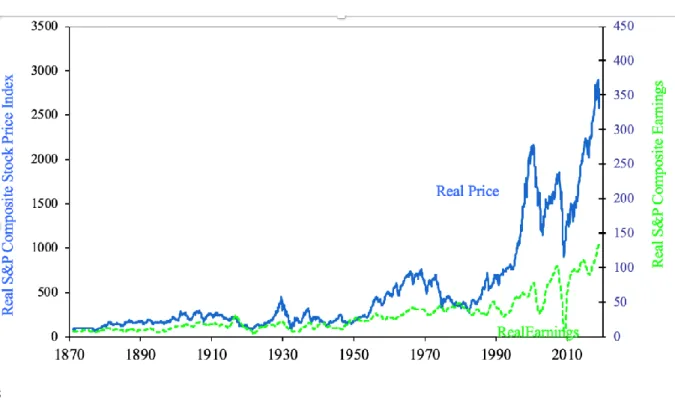
It seems quite difficult to say if the results that appeared sometime after were directly due to the effectiveness of the QE, but one fact is that the S&P500 index have been experiencing one of the strongest bull-markets ever, as can be observed in figure 1. Since 2009, the S&P500 index has been roaring ahead much beyond the previous maxima, not only nominal but also real ones.
Figure 1: Real monthly prices of the S&P500 index.
Nonetheless, it seems important to highlight the fact that the current stock market behavior has been happening within a peculiar period. First, because this era has been characterized by a slower GDP recovery when compared with other post-recession periods in
12
the US2. In particular, when looking at the period before the Dotcom bubble, we can observe
an average annual real GDP growth rate of 3.53%, and 2.52% during the period prior to the Great Recession. Since July 2009 until March 2019, the real growth rate was just 2.11%. As it was argued by Taylor (2014) “this very severe recession was followed by an extremely disappointing recovery”. Second, as we have already mentioned this period is being characterized by the application of unconventional monetary measures.
In order to better analyze this stock markets’ behavior, we used Robert Shiller’s Price-Earnings Ratio approach also known as CAPE (Cyclically Adjusted Price-to-Price-Earnings Ratio) or P/E103.
It is important to note the fact that this ratio is a more consistent indicator to assess long financial performance since it allows smoothing the fluctuations on corporate profits driven by the business cycles, as the earnings can be volatile from year to year.
𝐶𝐴𝑃𝐸 𝑅𝑎𝑡𝑖𝑜 =𝑃𝑡
𝐸𝑡−11→𝑡−1
̅̅̅̅̅̅̅̅̅̅̅̅̅
⁄ (1)
As we can see through the previous equation, this ratio is defined by the current real stock price divided by the average of the last ten years of earnings per share (moving average), excluding the current period. Both variables are adjusted for inflation (Consumer Price Index (CPI)) in order to convert them to real values. It allows us to compare the consistency of share prices over time and to have a measure of stock market under or over valuation. Moreover, this indicator is also a good predictor of future stock market returns as we shall be able to expose in the last section of this dissertation.
2 Again, Gorton and Metrick (2012) support this point of view indicating that “recovery has been weak at best”. 3 Presented in the Robert Shiller’s book Irrational Exuberance (2000) -
13
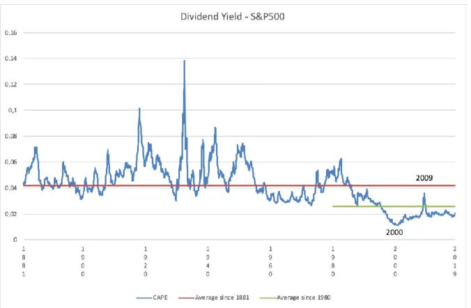
Figure 2: CAPE ratio of the S&P500 index.
As Robert Shiller mentioned4, it is important to look at historic data from which we
can extract since it is the main teacher concerning lessons of the financial booms and busts. Looking at the present situation, as we can see through the figure 2, it is possible to observe high current values (or by opposition, low earnings yield), when compared with other periods. Additionally, those are only lower than 1929 and 2000. It is important to recall that these two periods were considered two major bull-markets, that, as we could see, led to important price corrections. Taking into consideration a more recent period (since 1980), we also detect a persistent and significant discrepancy between the observed values and the average.
A rising CAPE ratio could be caused for other factors, real or erroneously perceived by investors. In this context it seems important to investigate what is driving this seemingly apparent disequilibrium.
Therefore, it is useful to decompose this ratio in order to understand the reason of this significant appreciation since 2009.
4 Financial Times interview – 2015.
14
Figure 3: Real S&P500 index prices versus Real Earnings of the S&P500 index.
5
As it is perceptible by the figure 3, both the real prices and the real earnings per share have been increasing since 2009 but the former faster than the latter. This can mean that prices are being influenced by some external variable other than the real earnings.
Simultaneously, it seemed also important to look at the length of the period in question. If it was a shorter period, this increase in the real prices, and consequently in the CAPE ratio, might be due to some occasional events. However, the effects have been persisting for almost ten years.
Immediately, looking at the significant CAPE ratio mostly driven by an important increase of the real stock prices and associated to a considerable duration of ten years, the question that came to our mind was the reason behind this abnormal behavior. In other words, what are the other structural drivers that are triggering this effect?
Thus, in this dissertation we try to search for some clues about the stock market behavior of the present period looking at some important structural macroeconomic variables – the economic activity, the monetary policy impact and the companies’ financial performance.
15
The approach of this dissertation is sustained on a specific research question: was there any structural change in the causality between macroeconomic and the stock’s market performance since 2009, perhaps caused by the influence of the unconventional monetary policy implemented in the US during the period under study?
In order to address this question, we decided to divide this dissertation in three sections. The first looks at the impact of the monetary policy surprise announcements on the stock markets. The second tests the relation among the four variables – economic activity, monetary policy, companies’ financial performance and real stock returns. Finally, we use a well-known stock-market forecasting model based on the notion of excess stock market returns in order to look at the S&P500 index overvaluation path.
B. Motivation
“Markets can remain irrational longer than you can remain solvent.” – John Maynard Keynes.
The motivation of this dissertation lies in a tentative to better comprehend the behavior of the S&P500 equity index in the rather interesting period that followed the Great Financial Crisis (2008-2009) by addressing the relation between the stock market’s performance and macroeconomic variables, namely economic activity and the monetary policy. The objective is to compare the relation across other periods of expansion and try to identify either similarities or differences with the current period.
In order to approach our goal, we decided to start by an introductory model that captures the direct impact of the monetary policy in stock markets. With this, we can show the significant relation between the two variables, what leads us to give a central role to monetary policy in our modelling strategy.
Having said that, we pursued our approach studying the relation among four important variables – economic activity, monetary policy, companies’ financial performance and stock markets. This is to say, to study the S&P500 index behavior through these indicators, as it was already said.
16
Finally, having some clues about this relation, we decided to simulate the current excess returns of the S&P500 index under recent past behavior (1951-2009) in order not only to capture the gap between the forecasted values and the actual ones as well as the forecasted path for the next five years.
However, we are aware of the limitations of our approach and more work needs to be done in order to conceptualize the impacts that we are going to try to identify, in the next sections.
C. A review of the relevant literature
Due to great improvements within the financial area, it is common knowledge among economists that the stock market is a significant variable for the economy and monetary policy but is also subject to their influence.
Therefore, in line with our dissertation focus, we decided to divide the literature review in two distinct parts. Firstly, we illustrate the relation between the stock markets and the economic activity. Afterwards, we address the relation between the stock markets and monetary policy (and its side effects).
This body of literature will help framing the approach followed in this dissertation, including the impact of the unconventional policies conducted since the Great Financial Crisis (GFC).
Relation between stock markets and economic activity:
Fama (1981), started by arguing about the positive correlation between real stock returns and real activity. A few years later, Fama (1990), identified that the future growth rates of industrial production, used as proxy for expected cash-flows, were responsible for 43% of the return variance of annual returns on the value-weighted portfolio of New York Stock Exchange (NYSE) between 1953 and 1987. Moreover, Schwert (1990) sustained and complemented this latter point using a longer period (1889-1988). Giving continuity to this reasoning, Barro (1990) exposed the significant positive correlation between the stock prices and the growth rate of the US aggregate business investment. In addition, Chen, Roll and
17
Ross (1986) tested positively the impact of innovations, in macroeconomic variables, on stock markets. They found significant results for: spread between long and short interest rates, expected and unexpected inflation, industrial production, and the spread between high and low-grade bonds. Moreover, Fama and French (1989) achieved the conclusion that “expected returns are lower when economic conditions are strong and higher when conditions are weak”. In addition, Cochrane (1991) approached the idea of forecasting noticing that “stock returns forecast real variables including investment and GNP”, also shared by Fischer and Merton (1982).
In the same line, Levine (1996) identified that the stock markets seemed to give a great boost to economic development, through the creation of liquidity even after multiple regressions controlling for inflation, fiscal policy, political stability, education, the efficiency of the legal system, exchange rate policy, and openness to international trade. According to this idea, Levine and Zervos (1996) concluded that stock market development is positively and robustly correlated with long-run economic growth, in spite of other studies that had demonstrated the opposite. Finally, it is important to underline the fact that stock markets were important during the period of the 1985-1999, since they represented 33% of the total financial wealth in the US, as it was approached by Rigobon and Sack (2003).
Finally, Lee (1992) approached this inverse relation stating that stock returns “appear Granger-causality prior” and, in this way, explain real activity. In the same line, Bernanke and Gertler (1999, 2001) argued that stock prices have a direct effect on output. A few years earlier (1989), the same authors have mentioned the point of the net worth of the entrepreneurs and its importance on the propagation of shocks to the economy.
Relation between stock markets and monetary policy impact:
Bjørnland and Leitemo (2009) showed a huge negative interdependency between the interest rate setting and real stock prices. In the same vein, Thorbecke (1997), Rigobon and Sack (2003 and 2004) and Bernanke and Kuttner (2005), identified a significant impact of the monetary policy (through the interest rate) on the equity markets. In other words, expansionary monetary policy leads to positive stock returns. Therefore, Kuttner (2001) detailed into a deeper perspective this effect and showed that the responses to a “surprise component” of the FED policy is significantly stronger than the response to the change itself,
18
which seems to continue aligned with the actuality. This will be the focus of our first empirical analysis in Section 2.
In parallel, it is also important to have in mind the view that indicates that the stock markets represent an important source of information for the conduction of the monetary policy, given by the authors Bjørnland and Leitemo (2009). Taking an alternative approach, Vickers (1999) concluded that asset prices matter for monetary policy in the way that they help to inform judgements about inflation prospects, while advising against including asset prices in the measure of the inflation targeted. Gilchrist and Leahy (2002) also argued against the inclusion of stock markets variables in the monetary policy making, explaining that asset prices tend to be positively correlated with movements in output and inflation, and so policies based on these variables will affect indirectly the financial markets. Conversely, Alchian and Klein (1973) argued for an inclusion of the asset prices in order to achieve a correct measure for inflation since “they reflect the current money prices of claims on future, as well as current, consumption”.
Additionally, concerning the unconventional monetary measures impact and learning with past events, Kimura and Small (2004) argued that the “quantitative monetary easing” undertaken by the Bank of Japan in 2001, aimed at increasing risk premia on assets with pro-cyclical returns such as equities. In the same line, Rogers, Scotti and Wright (2014) called our attention to the significant reduction of the term premia of the asset-market during the period of unconventional measures led by the FED and other Central Banks. Within the same rational, Bhattarai and Neely (2016) presented evidence of the US QE impact on the financial markets, namely equities having influenced in the desired manner. Moreover, Rosa (2012) exposed the facts for a high significance of those measures on asset prices, even after controlling for the surprise component of the FED’s communication about the future path. Hattori, Schrimpf and Sushko (2016) suggested that these measures seem to have a stabilizing and stimulatory effect on financial markets. In addition, Mishkin (2009) showed the importance of the monetary policy during the financial crisis in reducing the macroeconomic risk through lowering the interest rates on default-free securities and also on the credit spreads.
19 o Monetary policy and its side effects:
Despite, the at the time Chairman of the FED, Ben Bernanke, was conscious about the uncertainty of the monetary policies effects and the certainty about its costs. Concluding, in 2012, he argued that monetary policy was not as effective as economic policies and could not neutralize the “fiscal and financial risk” that a country can face.
Galí (2014) stated that “monetary policy cannot affect the conditions for existence (or non-existence) of a bubble, but it can influence its short-run behavior, including the size of its fluctuations”. Similarly, Bordo and Landon-Lane (2013) argued about the positive impact of the expansionary monetary policy (interest rate below the target rate) on asset prices and their subsequentially correction. In addition to that, Blanchard and Watson (1982) exposed the significant real impact of a financial market bubble on the economy.
2. A proxy for the monetary policy impact
As it was addressed in the literature review, the monetary policy seems to have a significant impact on financial markets, namely in the stock markets, and the other way around is also true.
Moreover, it is known that stock markets react, namely in the short run, to the expectations of the monetary policy set by the central bank and do not wait for the implementation of the announcements. This is in line with what was argued by D’Amico and King (2013) when they state that the effect of unconventional monetary policies is probably felt with announcements that are able to change market expectations. Thus, the US stock market, namely the S&P500 index, should not be an exception.
In order to start our analysis, we decided to set an estimation with the objective of observing the “immediate” impact of monetary policy announcements on the stock markets. In other words, to establish the relation of the investors’ anticipation within the S&P500 index to the FED announcements.
20
A. The data
For this and the following models (except for the last section of this dissertation), we shall use data from April 1991 until March 2019, divided into three periods of expansion. Those are, for the NBER, limited by the three recessions:
- July 1990 until March 1991 - March 2001 until November 2001 - December 2007 until June 2009 Therefore, the periods analyzed are:
- April 1991 until February 2001 - December 2001 until November 2007 - July 2009 until March 2019
It seems important to refer the fact that for this first analysis we decided to use daily data with the objective of having a more refined view of the FED surprise announcements.
Moreover, for this model, we shall use the absolute returns variations of the S&P500 index as dependent variable and absolute variations of the Treasury Bill for 6 Months (T-Bill 6M) interest rate as explanatory variable, both in nominal values. This “forward-looking” instrument is a valuable proxy to track monetary policy since, looking at the data, we assume this is one possible way how investors anticipate possible changes in the FED policy or react to actual FED surprise policy announcements. This because a shorter term is more lied to the establishing of the monetary policy and a higher term looks more at the state of the economy.
B. The model
In order to address this issue, we decided to use a binary (0;1) model resorting to the logistic regression (logit).
Recall that our objective is to analyze the direct effect of the FED surprise monetary policy on the stock returns of the S&P500 index. For that purpose, we decided to use the following model:
21
Where, 𝑆𝑅𝑡 refers to the nominal stock returns of the S&P500 index, and 𝐷𝑃𝑥𝑡 (x=1,2) to the dummy variables described below.
Defining our variables, we have:
𝑆𝑅𝑡= {1, 𝑖𝑓 | 𝑆&𝑃500𝑡 𝑆&𝑃500𝑡−1 − 1| > 𝑆𝑇𝐷𝐸𝑉(| 𝑆&𝑃500𝑡 𝑆&𝑃500𝑡−1 − 1|) 0, 𝑜𝑡ℎ𝑒𝑟𝑤𝑖𝑠𝑒 𝐷𝑃1𝑡 = { 1, 𝑖𝑓 |𝑇 − 𝐵𝑖𝑙𝑙 6𝑚𝑡 − 𝑇 − 𝐵𝑖𝑙𝑙 6𝑀𝑡−1| > 𝑆𝑇𝐷𝐸𝑉(|𝑇 − 𝐵𝑖𝑙𝑙 6𝑚𝑡 − 𝑇 − 𝐵𝑖𝑙𝑙 6𝑀𝑡−1|) 𝑎𝑛𝑑 |𝑇 − 𝐵𝑖𝑙𝑙 6𝑚𝑡 − 𝑇 − 𝐵𝑖𝑙𝑙 6𝑀𝑡−1| < 2 × 𝑆𝑇𝐷𝐸𝑉(|𝑇 − 𝐵𝑖𝑙𝑙 6𝑚𝑡 − 𝑇 − 𝐵𝑖𝑙𝑙 6𝑀𝑡−1| 0, 𝑖𝑓 𝑜𝑡ℎ𝑒𝑟𝑤𝑖𝑠𝑒 ) 𝐷𝑃2𝑡 = {1, 𝑖𝑓 |𝑇 − 𝐵𝑖𝑙𝑙 6𝑚𝑡 − 𝑇 − 𝐵𝑖𝑙𝑙 6𝑀𝑡−1 | > 2 × 𝑆𝑇𝐷𝐸𝑉(|𝑇 − 𝐵𝑖𝑙𝑙 6𝑚𝑡 − 𝑇 − 𝐵𝑖𝑙𝑙 6𝑀𝑡−1|) 0, 𝑖𝑓 𝑜𝑡ℎ𝑒𝑟𝑤𝑖𝑠𝑒
Where, STDEV refers to the standard deviation of the period analyzed (previously described).
It is important to note the fact that we are using absolute values in order to keep not only the positive changes but also the negative ones of the T-Bill 6M.
Moreover, in this model, we decided to split these absolute changes, through the standard variations, in two parts. In this way, we are assuming that important changes in the monetary policy expectations are, at least, twice of the standard deviation of the T-Bill 6M during the period in question.
C. The results
The results obtained through our econometric regression model are in line with what was expected.
However, before we start stating the results obtained, it is important to underline the facts that, on the one hand , the 𝑅2 is not very significant for our analysis and, on the other
22
ratio”6. For that reason, only the signal is interpreted and not the magnitude of the coefficient.
In other words:
If the coefficient is positive, it means that a rise in the explanatory variable increases the likelihood that the dependent variable is equal to 1.
On the contrary, if the coefficient is negative it means that an increase of the explanatory variable decreases the likelihood that the dependent variable is equal to 1. We can now look at our results, presented in the table below:
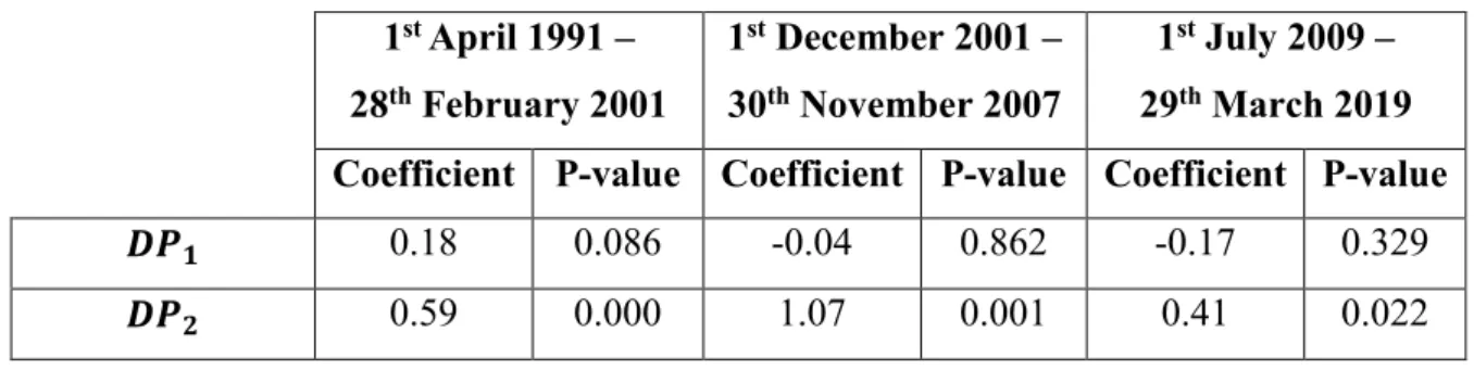
Table 1: Output of the Logit model, between April 1991 and March 2019.
1st April 1991 – 28th February 2001 1st December 2001 – 30th November 2007 1st July 2009 – 29th March 2019 Coefficient P-value Coefficient P-value Coefficient P-value
𝑫𝑷𝟏 0.18 0.086 -0.04 0.862 -0.17 0.329
𝑫𝑷𝟐 0.59 0.000 1.07 0.001 0.41 0.022
These results suggest that the stock market is subject to a significant impact of the monetary policy surprises announcements (in our model defined as 𝐷𝑃2). This is to say that,
using our proxy regarding the intervention of the monetary policy in the investors’ expectations, the stock returns are more likely to react. In other words, facing an event that makes the rate on the T-Bill 6M to vary by more than twice the standard deviation (for the period in question), the stock returns are more likely to change significantly (by more than one-standard deviation as per the definition of the dependent variable). Although, it is important to mention that this is just a proxy and T-Bills can move for other reasons.
This result complements the two following models in the sense that it suggests a significant impact of the monetary policy on the stock markets.
23
3. The macroeconomic relation
As it was observable in this first part and in line with the literature review, monetary policy is a significant variable when we are addressing stock returns variance.
Being our objective to address the stock market behavior since 2009 through macroeconomic relations, it seems important to include as variables, not only, the economic activity as well as some measure of monetary policy. Moreover, in order to complement and sustain the validity of the economic activity results set by the first model of this section, we decide to address another relation using the earnings of the companies of the S&P500 index.
A. The data
As it was already said, for the four following models7, we shall use data from April
1991 until March 2019, but now in a monthly basis, divided into the same three periods of expansion, previously defined.
In this way, the four variables chosen to approach the two VAR models, presented in this chapter, were the following: Industrial Production Index (IPI), the Effective Federal Funds Rate8 (substituted by the Wu-Xia Shadow Rate9 during the period of unconventional
measures), the real earnings per share of the companies that compose the S&P500 index, and the real prices of the S&P500 index.10
The Industrial Production Index11 is used in order to measure the economic activity
impact (characterized by the real Gross Domestic Product (GDP))12. We shall use the
7 The output of the other models is presented in the Appendix.
8 A possible measure to capture the impact of the monetary policy effectiveness. Tests with the T-Bill 6M variable were also performed and the output obtained was quite similar (results can be assessed in the Appendix).
9 Henceforth explained.
10 The ISM Index will also be used as a complementary approach of the IPI variable in order to give consistency to the first performed VAR (results can be assessed in the Appendix).
11 FRED definition: This index is an economic indicator that measures real output for all facilities located in the United States manufacturing, mining, electric, and gas utilities (excluding those in U.S. territories).
12 This dissertation is totally aware of the fact that the IPI is a proxy and industry does not represent the economy as a whole.
24
IPI year on year (YoY) growth rate in order to have a monthly measure highly correlated with the real GDP Growth YoY (through figure 4 it is possible to observe the data frequency between the two variables). Since our objective is to study the performance, we decided to use growth rates YoY.
Figure 4: The relation between the growth rates of the Industrial Production Index and the real Gross Domestic Product, year on year.
Right axis: Real GDP Growth YoY Left axis: IPI Growth YoY
The real GDP is one variable frequently used in order to represent the economy. However, we are aware of the limitations and problems of this indicator.
In parallel, the Purchasing Managers’ Index (PMI) from the Institute for Supply Management (ISM), also denoted ISM Index13, will be also used as a proxy to real
GDP Growth YoY in order to support our analysis with the IPI Index. As we can see
13 Quandl definition - composite index based on the diffusion indexes of five of the indexes with equal weights: New Orders (seasonally adjusted), Production (seasonally adjusted), Employment (seasonally adjusted), Supplier Deliveries (seasonally adjusted), and Inventories.
-.16 -.12 -.08 -.04 .00 .04 .08 .12 .16 .20 -.06 -.04 -.02 .00 .02 .04 .06 .08 .10 1980 1985 1990 1995 2000 2005 2010 2015
25
through the figure below, this indicator is also highly correlated with the real GDP growth rate.
Figure 5: The relation between the ISM Index and the real Gross Domestic Product growth rate year on year.
Right axis: Real GDP Growth YoY Left axis: ISM Index
The variable Effective Federal Funds Rate14 is used in order to account for the
monetary policy impact. The reason why it was chosen is the high correlation with the Federal Funds Target Range, as we can see through the figure 615.
Thus, during the period of unconventional monetary measures the impact is measured through the Wu-Xia shadow rate (from January 2009 until November 2015).16
14 The effective federal funds rate is the interest rate at which depository institutions trade federal funds (balances held at Federal Reserve Banks) with each other overnight.
15 This proxy was firstly approached by Bernanke, B and Blinder, A (1992).
16 This shadow rate will not suffer more updates as long as target range for the federal funds rate is at or above 25 to 50 basis points. The reason behind is the high correlation between the Wu-Xia rate and effective federal funds rate for levels of the former set at least at 25 basis points.
10 20 30 40 50 60 70 80 -.06 -.04 -.02 .00 .02 .04 .06 .08 .10 1980 1985 1990 1995 2000 2005 2010 2015
26
Figure 6: The relation between the Effective Federal Funds Rate and the Federal Funds Targets.
17
Figure 7: Wu-Xia Shadow Federal Funds Rate.
18
As we can see through the figure 7, during the Quantitative Easing, the rate is negative due to the set of unconventional measures.
The earnings are represented by the real earnings per share of the companies that belong to the S&P500 index and are used in order to track the profitability/performance of the same. In order to have stationarity and to track performance, we decided to apply the growth rate year on year of this variable.
17 Federal Reserve of St. Louis (FRED) - https://fred.stlouisfed.org/series/DFEDTARU#0
27
The stock markets are represented by the S&P500 index through the real stock returns growth rate year on year of the same index. Again, since our objective is to track the performance of the variables, having stationarity, we decided to use growth rate year on year.
These two last variables are deflated through the Consumer Price Index (CPI) in order to approach the real values.
B. A first approach
i.
The model
In order to study the real economic and monetary impacts on the stock markets (more precisely the S&P500 index) we decided to estimate a Vector Auto-Regression (VAR) model. The main reasons were the endogeneity between the three variables and, giving this reality, to have the possibility of subjecting these to structural shocks and, more important, to be able to analyze them. This is in line with what Lee (1992) argued about the usefulness of a VAR approach for investigating the relationship between stock returns and other variables.
The generic model can be presented with the following notation:
{ 𝐼𝑃𝐼𝑡 = 𝐶1+ 𝑎111 𝐼𝑃𝐼𝑡−1+ 𝑎121 𝐹𝐸𝐷𝑡−1+ 𝑎131 𝑆𝑅𝑡−1+ . . . +𝑎11 𝑝 𝐼𝑃𝐼𝑡−𝑝+ 𝑎12 𝑝 𝐹𝐸𝐷𝑡−𝑝+ 𝑎13 𝑝 𝑆𝑅𝑡−𝑝+ 𝜀1𝑡 𝐹𝐸𝐷𝑡 = 𝐶2+ 𝑎211 𝐼𝑃𝐼𝑡−1+ 𝑎221 𝐹𝐸𝐷𝑡−1+ 𝑎231 𝑆𝑅𝑡−1+ . . . +𝑎21 𝑝 𝐼𝑃𝐼𝑡−𝑝+ 𝑎22 𝑝 𝐹𝐸𝐷𝑡−𝑝+ 𝑎23 𝑝 𝑆𝑅𝑡−𝑝+ 𝜀2𝑡 𝑆𝑅𝑡 = 𝐶3+ 𝑎311 𝐼𝑃𝐼𝑡−1+ 𝑎321 𝐹𝐸𝐷𝑡−1+ 𝑎331 𝑆𝑅𝑡−1+ . . . +𝑎31 𝑝 𝐼𝑃𝐼𝑡−𝑝+ 𝑎32 𝑝 𝐹𝐸𝐷𝑡−𝑝+ 𝑎33 𝑝 𝑆𝑅𝑡−𝑝+ 𝜀3𝑡 ,
Where 𝐼𝑃𝐼𝑡 refers to IPI growth rate YoY (IPI YoY), and 𝐹𝐸𝐷𝑡 to effective federal (Fed) funds rate, and 𝑆𝑅𝑡 to real stock returns YoY.
Transforming in matrix notation, we have:
[ 𝐼𝑃𝐼𝑡 𝐹𝐸𝐷𝑡 𝑆𝑅𝑡 ] = [ 𝐶1 𝐶2 𝐶3 ] + [ 𝑎111 𝑎121 𝑎131 𝑎211 𝑎221 𝑎231 𝑎311 𝑎 32 1 𝑎 33 1 ] [ 𝐼𝑃𝐼𝑡−1 𝐹𝐸𝐷𝑡−1 𝑆𝑅𝑡−1 ] + . . . + [ 𝑎11𝑝 𝑎12𝑝 𝑎13𝑝 𝑎21𝑝 𝑎22𝑝 𝑎23𝑝 𝑎31𝑝 𝑎32𝑝 𝑎33𝑝 ] [ 𝐼𝑃𝐼𝑡−𝑝 𝐹𝐸𝐷𝑡−𝑝 𝑆𝑅𝑡−𝑝 ] + [ 𝜀1𝑡 𝜀2𝑡 𝜀3𝑡 ]
28 Therefore, the reduced form can be written as:
𝐴(𝐿)𝑌𝑡 = 𝜀𝑡
Where, 𝐴(𝐿) = 1 − 𝐴1𝐿 − 𝐴2𝐿2 − 𝐴3𝐿3− . . . −𝐴𝑝𝐿𝑝
Being L the lag operator and 𝑌𝑡 the matrix formed by the three variables that belong to our model.
Assuming that this process is stationary (this means no unit root), we can write this equation as:
𝑌𝑡 = 𝐴−1(𝐿)𝜀𝑡
In order to be able to submit the three variables of the model to structural shocks from each of them, we decided to transform the VAR in a Structural Vector Auto-Regression (SVAR), resorting to the Cholesky decomposition.
Therefore, following the Cholesky approach, the reduced model can be written as: 𝑌𝑡 = 𝐴−1(𝐿)𝐶𝜇𝑡
The C matrix is inferior diagonal and can be written as:
𝐶 = [
𝑆11 0 0
𝑆21 𝑆21 0
𝑆31 𝑆32 𝑆33 ]
Moreover, 𝜇𝑡 is the error matrix composed by the structural shocks. The construction of the
latter needs to be carefully developed since the order of the variables is highly significant for the results.
In this case, we decided to have the following order19:
𝜇𝑡 = [
𝜇𝐼𝑃𝐼𝑡
𝜇𝐹𝐸𝐷𝑡
𝜇𝑆𝑅𝑡 ]
Here we are assuming that the Industrial Production Index reacts immediately only to its own shock. An example of this shock can be a productivity shock in the economy.
29
In the same line, the Effective Federal Funds Rate reacts immediately both to a shock to the IPI and to its own shock. An example of the latter can be a surprise interest rate increase by the FED.
Finally, the Stock Returns react immediately not only to its own shock as well as to the IPI and effective federal funds rate shocks. An example of an own shock within the S&P500 index can be a re-appraisal of the multiples (also called Price-Earnings ratio). With this movement, investors will expect more (or less) for 1 unit of the earnings tomorrow, depending on whether we are in presence of a positive (or negative) shock.
Therefore, we can write our econometric regression model as:
[ 𝐼𝑃𝐼𝑡 𝐹𝐸𝐷𝑡 𝑆𝑅𝑡 ] = 𝐴−1(𝐿) [ 𝑆11 0 0 𝑆21 𝑆22 0 𝑆31 𝑆32 𝑆33 ] [ 𝜇𝐼𝑃𝐼𝑡 𝜇𝐹𝐸𝐷𝑡 𝜇𝑆𝑅𝑡]
ii.
Robustness of the model
The robustness of this model was studied through the performance of one complement VAR that includes the ISM Index instead of the IPI YoY, as primarily mentioned. The results obtained through this variable are similar to the ones that we shall present and are available in the appendix. Moreover, another test was performed with the T-Bill 6M instead of the Effective Federal Funds Rate variable and the results were also quite similar. The similarity reinforces the consistency of the results achieved in our previous model.
Yet, it could be the case that some variables are not stationary although we should be aware that this is not a problem since without cointegration among the variables used, the VAR model continues to be well specified. Nevertheless, the VAR satisfies the stability condition for all the sub-periods analyzed, a necessary condition to the robustness of our model.
30
iii.
The results
The lag length of the model is supported by the five criteria presented on the EViews program – Sequential modified likelihood ratio, Final prediction error, Akaike information criterion, Schwarz information criterion, Hannan-Quinn information criterion.
The importance of the lag length is well stressed by Braun and Mittnik (1993), which showed the fact that when lag length in a VAR model is different from the true lag length, the estimates are inconsistent as well as the respective impulse-response functions and variance decomposition. Similarly, Lütkepohl (1993) indicates that an overfitting, in other words, a higher order lag length than the true lag length causes an increase in the mean-square forecast errors. In the same line, an underfitting of the lag length often generates autocorrelated errors.
The results are presented in the form of impulse-response functions to shocks in each of the VAR variables. It is important to clarify that the measures are in percentage points. This means that a x percentage point increase in a variable lead to an y percentage point variation in the other variable.
It should be recalled that the objective of this model is to uncover the relation between the three variables in the most recent period (July 2009 – March 2019) comparing with the other previous periods of expansion, in order to track the current bull market of the S&P500 index. For that, we analyze each of the periods in turn.
31 a) April 1991 until March 2019
Output Figures 1: Impulse-Response Functions of the three variables (IPI growth rate YoY, effective federal funds rate, real stock returns YoY) by the Cholesky decomposition, between April 1991 and March 2019. -0. 4 0.0 0.4 0.8 5 10 15 20 25 30 35 40 45 50 55 60 R es po ns e of IP I_ Y O Y to I P I_ Y O Y -0. 4 0.0 0.4 0.8 5 10 15 20 25 30 35 40 45 50 55 60 R es po ns e of I P I_ Y O Y t o E FF E C TI V E _F E D _F U N D S _R A TE -0. 4 0.0 0.4 0.8 5 10 15 20 25 30 35 40 45 50 55 60 R es po ns e of I P I_ Y O Y t o R E A L_ S TO C K _R E TU R N S _Y O Y -.1 .0 .1 .2 .3 .4 .5 5 10 15 20 25 30 35 40 45 50 55 60 R es po ns e of E FF E C TI V E _F E D _F U N D S _R A TE t o IP I_ Y O Y -.1 .0 .1 .2 .3 .4 .5 5 10 15 20 25 30 35 40 45 50 55 60 R es po ns e of E FF E C TI V E _F E D _F U N D S _R A TE t o E FF E C T IV E _F E D _F U N D S _R A T E -.1 .0 .1 .2 .3 .4 .5 5 10 15 20 25 30 35 40 45 50 55 60 R es po ns e of E F FE C T IV E _F E D _F U N D S _R A TE t o R E A L_ S TO C K _R E TU R N S _Y O Y 0 2 4 6 5 10 15 20 25 30 35 40 45 50 55 60 R es po ns e of R E A L_ S TO C K _R E TU R N S _Y O Y t o IP I_ Y O Y 0 2 4 6 5 10 15 20 25 30 35 40 45 50 55 60 R es po ns e of R E A L_ S TO C K _R E T U R N S _Y O Y t o E F FE C T IV E _F E D _F U N D S _R A TE 0 2 4 6 5 10 15 20 25 30 35 40 45 50 55 60 R es po ns e of R E A L_ S TO C K _R E T U R N S _Y O Y t o R E A L_ S TO C K _R E TU R N S _Y O Y R es po ns e to C ho le sk y O ne S .D . ( d. f. ad ju st ed ) I nn ov at io ns – 2 S .E .
32
The results seem to be aligned with what is usually argued in the economic literature as showed in our literature review, though with some exceptions.
Starting by these exceptions, namely the monetary policy impact, it is observable that the responses of the IPI YoY and the real stock returns YoY to a positive shock in the variable effective federal funds rate are not intuitive. Thus, the results should be read with caution since zero is inside the confidence bands. So, upon a 1 percentage point increase of the interest rate (tightening of the monetary policy), the economic activity seems to increase 0.2 percentage points in the short run (after 1,5 years). Regarding the stock market, it is possible to observe that a tightening of the monetary policy seems to have a negative impact in the short-term but quickly compensated in the medium-term. A result that might warrant more work in order to interpret this unintuitive outcome.
Besides, we can observe a positive correlation between the economic activity and the real stock returns, knowing that the impact of the latter on the economic activity is smaller and slower than the opposite. This result is in line with the conclusion set in our literature review.
In other words, the positive response of the IPI YoY to a 1 percentage point increase of the real stock returns is set at 0.8 percentage points in 1 year. The opposite follows the same tendency but with different magnitudes. For a 1 percentage point increase of the IPI YoY, the real stock returns tend to increase around 1.5 percentage points during the firsts 6 months.
Another interesting finding is the reaction of the monetary policy when the economic activity and stock market are improving. This means, upon a 1 percentage point increase of the IPI YoY, the effective federal funds rate tends to increase around 0.1 percentage points. The same relation is also true to a positive shock in real stock returns YoY. This can give us some ideas about the behavior of the FED, which tends to increase the interest rate when economic conditions are good until a certain point.
33 b) April 1991 until February 2001
Output Figures 2: Impulse-Response Functions of the three variables (IPI growth rate YoY, effective federal funds rate, real stock returns YoY) by the Cholesky decomposition, between April 1991 and February 2001. -.4 -.2 .0 .2 .4 .6 5 10 15 20 25 30 35 40 45 50 55 60 R es po ns e of IP I_ Y O Y to I P I_ Y O Y -.4 -.2 .0 .2 .4 .6 5 10 15 20 25 30 35 40 45 50 55 60 R es po ns e of I P I_ Y O Y t o E FF E C TI V E _F E D _F U N D S _R A TE -.4 -.2 .0 .2 .4 .6 5 10 15 20 25 30 35 40 45 50 55 60 R es po ns e of I P I_ Y O Y t o R E A L_ S TO C K _R E TU R N S _Y O Y -.1 .0 .1 .2 5 10 15 20 25 30 35 40 45 50 55 60 R es po ns e of E FF E C TI V E _F E D _F U N D S _R A TE t o IP I_ Y O Y -.1 .0 .1 .2 5 10 15 20 25 30 35 40 45 50 55 60 R es po ns e of E FF E C TI V E _F E D _F U N D S _R A TE t o E FF E C T IV E _F E D _F U N D S _R A T E -.1 .0 .1 .2 5 10 15 20 25 30 35 40 45 50 55 60 R es po ns e of E F FE C T IV E _F E D _F U N D S _R A TE t o R E A L_ S TO C K _R E TU R N S _Y O Y -2 0 2 4 5 10 15 20 25 30 35 40 45 50 55 60 R es po ns e of R E A L_ S TO C K _R E TU R N S _Y O Y t o IP I_ Y O Y -2 0 2 4 5 10 15 20 25 30 35 40 45 50 55 60 R es po ns e of R E A L_ S TO C K _R E T U R N S _Y O Y t o E F FE C T IV E _F E D _F U N D S _R A TE -2 0 2 4 5 10 15 20 25 30 35 40 45 50 55 60 R es po ns e of R E A L_ S TO C K _R E T U R N S _Y O Y t o R E A L_ S TO C K _R E TU R N S _Y O Y R es po ns e to C ho le sk y O ne S .D . ( d. f. ad ju st ed ) I nn ov at io ns – 2 S .E .
34
In order to analyze the monetary policy impact in the stock markets it is important to contextualize the period. At the time, the Chairman of the FED, Allan Greenspan, led a policy of significant interest rate reduction between 1988 and 1992. After that, it was possible to observe a strong bull market of the stock markets and a significant recovery of the economy accompanied by a slight increase of the interest rates.
Starting with the monetary policy impact, the results indicate that a positive shock in the effective federal funds rate leads to a decrease of the real stock returns (almost 2 percentage points), in the short run. Conversely, expansionary monetary policy can lead to an appreciation of the real stock returns.
In the same line, the impact of a monetary policy shock in the economic activity seems also to be intuitive. This means that under a shock that leads to a 1 percentage point increase of the effective federal funds rate, the economic conditions will tend to decrease 0.2 percentage points, one year after.
However, the impact of the output growth on the stock markets seems to be less intuitive and not significant. This gives us some clues about the bubble that was forming at the time, meaning that the investors might have looked at other indicators beyond the economic activity. However, the converse makes more sense since for a 1 percentage point increase of the real stock returns YoY, the industrial output reacts with an almost 0.4 percentage points increase, one year after, what can sustain the arguments set in our literature review about the impact of the stock markets on the economic activity.
Besides, it is also possible to identify a similar interest rate behavior as the previous period already analyzed. In other words, for a positive shock in the IPI YoY (1 percentage point increase), the interest rates will tend to increase (almost 0.2 percentage points). The correlation between the stock market performance the monetary policy path seems to follow the same path but the relation should be read with caution since zero is inside the confidence bands. Again, this shows us that the Central Bank was likely to increase the interest rates when the economic activity is running well.
35 c) December 2001 until November 2007
Output Figures 3: Impulse-Response Functions of the three variables (IPI growth rate YoY, effective federal funds rate, real stock returns YoY) by the Cholesky decomposition, between December 2001 and November 2007. -.2 .0 .2 .4 .6 5 10 15 20 25 30 35 40 45 50 55 60 R es po ns e of IP I_ Y O Y to I P I_ Y O Y -.2 .0 .2 .4 .6 5 10 15 20 25 30 35 40 45 50 55 60 R es po ns e of I P I_ Y O Y t o E FF E C TI V E _F E D _F U N D S _R A TE -.2 .0 .2 .4 .6 5 10 15 20 25 30 35 40 45 50 55 60 R es po ns e of I P I_ Y O Y t o R E A L_ S TO C K _R E TU R N S _Y O Y -.1 .0 .1 .2 .3 5 10 15 20 25 30 35 40 45 50 55 60 R es po ns e of E FF E C TI V E _F E D _F U N D S _R A TE t o IP I_ Y O Y -.1 .0 .1 .2 .3 5 10 15 20 25 30 35 40 45 50 55 60 R es po ns e of E FF E C TI V E _F E D _F U N D S _R A TE t o E FF E C T IV E _F E D _F U N D S _R A T E -.1 .0 .1 .2 .3 5 10 15 20 25 30 35 40 45 50 55 60 R es po ns e of E F FE C T IV E _F E D _F U N D S _R A TE t o R E A L_ S TO C K _R E TU R N S _Y O Y -2 0 2 4 6 5 10 15 20 25 30 35 40 45 50 55 60 R es po ns e of R E A L_ S TO C K _R E TU R N S _Y O Y t o IP I_ Y O Y -2 0 2 4 6 5 10 15 20 25 30 35 40 45 50 55 60 R es po ns e of R E A L_ S TO C K _R E T U R N S _Y O Y t o E F FE C T IV E _F E D _F U N D S _R A TE -2 0 2 4 6 5 10 15 20 25 30 35 40 45 50 55 60 R es po ns e of R E A L_ S TO C K _R E T U R N S _Y O Y t o R E A L_ S TO C K _R E TU R N S _Y O Y R es po ns e to C ho le sk y O ne S .D . ( d. f. ad ju st ed ) I nn ov at io ns – 2 S .E .
36
In terms of results, let’s start with the unintuitive impact of the output shock on the stock market. We can observe that a 1 percentage point rise in IPI YoY generates a negative reaction of the real stock returns YoY during the firsts 6 months at around 2 percentage points. Again, this can mean that, at the time, other variables could be influencing the real stock returns rather than economic activity. Similarly, the converse relation is not obvious. Facing a 1 percentage point increase of the real stock returns YoY, the output decreases in the short run (during the first year) but rises over the medium-term. However, it is possible to observe a significant positive impact of the real stock returns on the ISM index.
It was no doubt, a period (before the Great Recession) where the stock markets increased significantly. Immediately after 2007, the stock markets started giving their first warnings (S&P500 index bear market) before the recession, even if the economy did not indicate the same. Confronting this with our results, the negative correlation between the two variables seems to make sense. Moreover, this is in line with the literature presented that indicates the stock market as a good predictor of the business cycles
When we consider the monetary policy impact, the results are not significant. This can give us some clues about the importance that investors took to this variable at the time.
Looking at the FED policy, the results are also not significant for the impact of economic activity. However, through our output, it is possible to observe a slight impact of the real stock returns on the FED policy. This means that for a 1 percentage point increase of the real S&P500 index, the effective federal funds rate tends to increase 0.05 percentage points. Yet, we are aware of the low significance of this result but this could indicate some influence of equity market performance on the policy followed at the time by the FED.
37 d) July 2009 until March 2019
Output Figures 4: Impulse-Response Functions of the three variables (IPI growth rate YoY, effective federal funds rate, real stock returns YoY) by the Cholesky decomposition, between July 2009 and March 2019. -.4 .0 .4 .8 5 10 15 20 25 30 35 40 45 50 55 60 R es po ns e of IP I_ Y O Y to I P I_ Y O Y -.4 .0 .4 .8 5 10 15 20 25 30 35 40 45 50 55 60 R es po ns e of I P I_ Y O Y t o E FF E C TI V E _F E D _F U N D S _R A TE -.4 .0 .4 .8 5 10 15 20 25 30 35 40 45 50 55 60 R es po ns e of I P I_ Y O Y t o R E A L_ S TO C K _R E TU R N S _Y O Y -.4 -.2 .0 .2 .4 .6 5 10 15 20 25 30 35 40 45 50 55 60 R es po ns e of E FF E C TI V E _F E D _F U N D S _R A TE t o IP I_ Y O Y -.4 -.2 .0 .2 .4 .6 5 10 15 20 25 30 35 40 45 50 55 60 R es po ns e of E FF E C TI V E _F E D _F U N D S _R A TE t o E FF E C T IV E _F E D _F U N D S _R A T E -.4 -.2 .0 .2 .4 .6 5 10 15 20 25 30 35 40 45 50 55 60 R es po ns e of E F FE C T IV E _F E D _F U N D S _R A TE t o R E A L_ S TO C K _R E TU R N S _Y O Y -2 0 2 4 5 10 15 20 25 30 35 40 45 50 55 60 R es po ns e of R E A L_ S TO C K _R E TU R N S _Y O Y t o IP I_ Y O Y -2 0 2 4 5 10 15 20 25 30 35 40 45 50 55 60 R es po ns e of R E A L_ S TO C K _R E T U R N S _Y O Y t o E F FE C T IV E _F E D _F U N D S _R A TE -2 0 2 4 5 10 15 20 25 30 35 40 45 50 55 60 R es po ns e of R E A L_ S TO C K _R E T U R N S _Y O Y t o R E A L_ S TO C K _R E TU R N S _Y O Y R es po ns e to C ho le sk y O ne S .D . ( d. f. ad ju st ed ) I nn ov at io ns – 2 S .E .
38
As previously mentioned, this period is in some way uncommon due to the unconventional monetary policies conducted by the Central Bank of the United States. At the same time, we have been witnessing a very long bull market despite the slow economic recovery when compared to other post-recessions periods. Therefore, the objective is to understand the difference among the dynamics of the three variables and try to identify some patterns about this period (2009-2019).
The first relevant result is the reaction of the stock markets to a shock in the output growth. In fact, a 1 percentage point increase of the latter gives rise to an increase of almost 2 percentage points of the former, during the firsts 6 months. In some way, we can see the fact that the economic activity is affecting the stock returns more significantly in the short run, when compared with the other periods analyzed. This can give us a clue about the sensitiveness of the stock markets during this period.
Moreover, the reaction of the output growth to a shock on the real stock returns seems to be similar to the other periods (except the period before the Great Recession). This means that the response of the IPI YoY to a real stock returns shock (1 percentage point increase) is almost 0.4 percentage points, during the first year.
Observing the monetary policy impact, we can see that the magnitude of the shocks in the effective federal funds rate is similar to the period before the Dotcom bubble. This means that an increase of 1 percentage point in the effective federal funds rate leads to a short-run decrease of the real stock returns YoY on almost 2 percentage points and 0.4 percentage points in the IPI YoY.
In addition, the neutral impact of the stock returns and the economic activity on the effective federal funds rate seems an interesting result. Looking at what happened, the FED only started increasing the interest rate in December 2015 what gives us a small number of observations. It seems acceptable, with the S&P500 index hitting maximum values, month after month, the economic activity growing and the interest rates at the zero-lower bound, that the relation effects are not significant.
Concluding this first subpart, it seems that monetary policy has having a significant direct impact not only on economic activity but also on the real stock returns of the S&P500 index in the current period. Finally, more work needs to be done in order to interpret the high
39
significant impact of a shock to the economic activity on the real stock returns when compared to the two previous periods of expansion where the model suggests low significance. The question that we can ask if it is the case that investors are paying more attention to the economic indicators, namely to the performance of the companies, or, on the contrary, the greater sensitivity of stock markets to activity indicators is an indirect impact coming through an amplification effect of changes in economic conditions by the unconventional monetary policy.
C. A different approach
i.
The model
Having assessed the relation between macroeconomic variables, a different approach, accounting for real earnings of the companies, was adopted in order to develop, support, and complement our previous econometric regression model. Looking at figure 3, we can notice that the real earnings per share are also reaching historic maximum values. Knowing this statement, we wanted to test if those are having a significant relation with the stock returns. In other words, if this variable is contributing for the S&P500 index behavior.
The model is quite similar to the previous one as well as the approach by the impulse-response functions. The main difference is the variable “real earnings growth rate YoY” instead of the “IPI growth rate YoY”.
The error matrix has the following order:
𝜇𝑡 = [
𝜇𝑅𝐸𝑡
𝜇𝐹𝐸𝐷𝑡
𝜇𝑆𝑅𝑡 ]
Where, 𝑅𝐸𝑡 refers to real earnings growth rate YoY (real earnings YoY), and 𝐹𝐸𝐷𝑡 to effective federal (Fed) funds rate, and 𝑆𝑅𝑡 to real stock returns YoY.
Here we are assuming that the Real Earnings variable reacts immediately only to its own shock. An example of this shock can be a technology shock that suddenly increases the
40
productivity of the companies. The other shocks were already explained in our previous econometric regression model.
Again, an important note should be made in order to enhance the fact that the three variables are endogenous among themselves.
Therefore, we can write our new model as:
[ 𝑅𝐸𝑡 𝐹𝐸𝐷𝑡 𝑆𝑅𝑡 ] = 𝐴−1(𝐿) [ 𝑆11 0 0 𝑆21 𝑆22 0 𝑆31 𝑆32 𝑆33 ] [ 𝜇𝑅𝐸𝑡 𝜇𝐹𝐸𝐷𝑡 𝜇𝑆𝑅𝑡 ]
ii.
Robustness of the model
The econometric regression satisfies the stability condition for all the periods that will be analyzed. This means that no roots lie outside the unit circle, a necessary condition for the robustness of our model.
iii.
The results
Again, the lag length is defined as the previous model using to the same five information criteria of the previous VAR model.
In this model, we shall focus on the relation between real earnings growth rate and real stock returns, both YoY, since the relation between the monetary policy and real stock returns appears to be quite similar to the model analyzed previously.
Once again, we shall analyze period by period in order to be able to have a critical view of the present period. Similarly, the results obtained by the impulse-response functions can be interpreted in the same way as the previous model.
41 a) April 1991 – March 2019
During the all sample analyzed (1991-2019), it is possible to identify a positive correlation, for both sides, between real stock returns and real earnings growth rate, what is in line with the results set in our previous model.
This means, that upon a 1 percentage point increase of the real earnings growth rate YoY, the reaction of the real stock returns is to increase almost 2 percentage points. The opposite is also true, with a response of 20 percentage points increase of the real earnings one year after the shock of a 1 percentage point increase of the real stock returns YoY. However, this last relation is compensated by a negative one in the medium term.
The first result is quite intuitive since if the companies are more profitable, they should be more valuable, which we see at least in the short term. Looking in particular at the second one, it would make sense if we assume that the investors are rational agents. This is in the sense that people are investing today because they are expecting an increase of the real earnings in a near future. Nevertheless, this is only a possible clue for the justification because of the limitations of our VAR model. A deeper analysis is needed in order to interpret consistently this result.
b) April 1991 – February 2001
Considering the period prior to the Dotcom bubble, the relation between the real earnings per share and the real stock returns is not so evident. This lack of clarity complicates the analysis that could be done.
However, the non-significant result presented in this output sustains our first analysis about the possibility of some other variable affecting the real stock returns of the S&P500 index.
Focusing on the response of the real earnings to a positive shock in the real stock returns can show us, in some way, the irrationality of the agents. In other words, this evinces that the agents invested, which led to a 1 percentage point of the real stock returns, against a null return.