The impact of major modes of climate variability on wave parameters in the western european coast

Resumo

O comportamento das ondas gravíticas superficiais oceânicas tem tido desde sempre um papel de grande importância na evolução geológica e socio-economica das regiões costeiras. Desde tempos pré-historicos as primeiras povoações humanas em regiões costeiras tiveram que enfrentar-se com a variabilidade das condições das ondas e com as consequências relativas. As condições de ondulação apresentam uma grande variabilidade espacial e temporal que tem um impacto directo na eficiência de várias atividades económicas, entre as quais podemos mencionar o transporte maritimo e a pesca. O conhecimento do clima das ondas pode ser de grande importância na transição para um modelo energético baseado em fontes de energia renováveis, entre as quais a energia gerada pelas ondas poderá ter um papel determinante. A erosão costeira é tambem fortemente relacionada com as características da ondulação. Nos ultimos anos as actividades económicas relativas ao turismo dos desportos de ondas são cada ano mais relevantes nas regiões costeiras europeias, em particular em Portugal, e dependem muito do regime de ondulação e da sua variabilidade no tempo (e.g. surf).

O objetivo central deste estudo é o de analisar a existência de uma ligação entre a variabilidade do clima das ondas e certos modos de variabilidade climática bem como avaliar o papel destes como possíveis predictores. Os modos climáticos em estudo são: Oscilação do Atlântico Norte (North Atlantic Oscillation, NAO), padrão do Atlântico Este (East Atlantic pattern, EA) e o padrão da Escandinávia (Scandinavian Pattern, SCAND), sendo que são tendencialmente considerados os padrões de circulação atmosférica a larga-escala mais importantes para o clima da região Euro-Atlântica.

Os dados referentes aos parámetros das ondas são relativos a dez pontos ao longo da costa Europeia e foram retirados de uma base de dados obtida através de um modelo de ondas regional que cobre a area do Atlántico Nordeste, produzido e validado por (Dodet et al., 2010). O modelo simula as condições de ondas a partir do modelo espectral WW3 forçado por uma reanalisis do campo do vento NCEP.

Os parametros de ondas usados neste trabalho são: a altura significativa da onda (Hs); a média da terça parte das ondas com maior altura registadas durante o tempo considerado; e periodo de pico (Tp): o periodo associado ao maior nível de

energia num grafico espectral. A partir destes dados foram calculadas médias interanuais relativas ao Inverno (Dezembro-Março) caracterizadas por um valor que representa a média de todos os registos desse conjunto de meses. As médias interanuais foram normalizadas subtraindo o valor médio e dividindo pelo desvio-padrão. A normalização dos dados permite compreender melhor a magnitude das anomalias presentes e desta forma distinguir mais facilmente valores normais de valores menos comuns das variáveis em estudo.

Os dados referentes aos modos clímaticos foram retirados do site do Climate Prediction Center (CPC) da NOAA (National Oceanic and Atmospheric Administration) para os mesmos períodos temporais dos dados das ondas, mas com uma resolução mensal: um valor de índice (por cada modo) por cada mês. Os índices foram calculados pela NOAA com recurso a uma análise PCA ao campo da altura geopotencial aos 500 hPa. A identificação das diferentes fases de cada modo foi feita com uma base no valor dos seus índices: a fase positiva é definida por um índice ≥ 0.5; a fase negativa por um índice de ≤ - 0.5; e a fase intermédia ou neutra por um índice entre 0.5 e -0.5. A partir dos índices dos modos clímaticos foram feitas médias interanuais e foram normalizadas da mesma forma usada pelos dados de onda.

Para avaliar o impacto dos modos climáticos com a variabilidade do clima das ondas foi feita uma comparação entre a variabilidade interanual das médias invernais dos parâmetros da onda escolhidos e dos modos climaticos. As correlações foram calculadas com o coeficiente de correlação de Pearson para um grau de significância de (p<0.10).

O resultado desta comparação revela que a variabilidade interanual da ondulação relativa ao inverno pode ser associada para uma grande parte da área em estudo com os índices da NAO, EA e SCAND. Encontraram-se correlações significativas entre os valores relativos à altura significativa da onda (Hs) e o índice da NAO em todos os pontos localizados entre 07.5º-02.5ºW e 50.0º-45.0N. A correlação entre NAO e Hs decresce de forma constante para sudoeste tornando-se negativa a sul dos 42.5ºN, até atingir correlações negativas fracas (mas estatisticamente significativas) nos dois pontos mais a sul (localidades 9 e 10). Correlações positivas e significativas foram encontradas tambem entre a NAO e o periodo de pico (Tp) em todos os pontos. EA-Hs e EA-Tp apresentam correlações positivas e significativas

em todos os pontos. SCAND e Hs têm correlações significativas nos pontos a sul de 42.5ºN e crescem até atingir o valor maximo de 0.39 na localidade mais a sul (localidade 10). Não foram encontradas correlações significativas entre SCAND e Tp.

O impacto dos modos clímaticos foi também estudado a partir da analise das distribuições de Hs e de Tp. Este estudo foi centrado nos pontos localizados mais a norte (1) e mais a sul (10) devido à grande diferença que mostraram na análise das correlações entre os parametros de onda e os índices dos modos climaticos. A significatividade das variações das distribuições foi avaliada com o teste de Kolmogorov-Smirnov. Encontrou-se que em 1 as fases positivas da NAO são significativamente associadas a uma distribuição da Hs mais larga e com valores médios mais altos que no caso da fase negativa da NAO. Tambem as fases da EA no ponto 1 têm um impacto significativo na distribuição de Hs parecido com o impacto da NAO. As mesmas correlações positivas foram encontradas para NAO e EA em relação ao Tp em 1. Não foram encontradas variações significativas em função das fases do índice SCAND para a distribuição da Hs e do Tp em 1. No ponto 10 (mais a sul) a distribuição da Hs tem uma fraca correlação negativa com a NAO mas as distribuições não são significativamente diferentes. Um impacto significativo e positivo foi encontrado para a EA e distribuição de Hs em 10. O impacto na distribuição de Tp é significativo e positivo para NAO e EA em 10. A influência da SCAND na distribuição de Hs e Tp em 10 apresenta variações fracas e não-significativas.

Os modos climáticos podem interagir entre si, resultando em estruturas espaciais modificadas. Por tal, uma avaliação do impacto destes na distribuição dos parametros de onda foi feita também para fases combinadas. Encontrou-se que a NAO e a EA têm um impacto significativo na distribuição de Hs quando se encontram na mesma fase e que anulam o impacto quando se encontram em oposição de fase no ponto 1. Contrariamente, a oposição das fases entre NAO e EA tem um impacto significativo em 10 onde são registadas Hs maiores durante a combinação de fases (NAO-EA+) e Hs mais pequenas durante (NAO+EA-). A influência das fases da SCAND também nesta análise é fraca e não-significativa. Por fim foi avaliada a capacidade de um modelo de regressão linearl (MLRM) para reconstruir a variabilidade das medias interanuais dos parâmetros das ondas

relatívas ao inverno a partir dos índices da NAO, da EA e da SCAND usados como variáveis predictoras. As séries reconstruidas apresentam correlações positivas e estatisticamente significativas com as séries originais com um valor máximo de 0.71 encontrado para a altura significativa da onda no ponto 10. Em conclusão, a partir dos resultados obtidos, é possivel afirmar que os modos de variabilidade climática NAO, EA e SCAND têm um impacto no clima das ondas nas costas europeias. NAO e EA mostraram as melhores correlações com os parametros de onda em todas as análises. O impacto da SCAND, a pesar de não ser notável nas análises das distribuições de Hs e Tp, deu correlações significativas e positivas com Hs só a a sul dos 42.5º, o que deixa aberta a hipótese de que melhores correlações possam encontrar-se ampliando a área de análise para latitudes mais baixas. Palavras-chave: Ondas gráviticas superficiais, Variabilidade Climatica, North Atlantic Oscillation (NAO), East Atlantic Pattern (EA), Scandinavian Pattern (EA)

Abstract

The North Atlantic Oscillation (NAO), the East Atlantic (EA) and the Scandinavian (SCAND) modes are three main large-scale circulation patterns driving the climate variability of the Euro-Atlantic region. This work evaluates their impact in wave climate parameters and assesses their skill as predictors of wave activity. The representative wave parameters used for this purpose are the significant wave height (Hs) and the peak period (Tp). Wave data have been retrieved from a 57-year hindcast study (1953–2009), obtained with the spectral wave model WW3 forced with the NCEP reanalysis of the wind fields, that was implemented and validated by (Dodet et al., 2010). This model provided wave data for 10 key locations that cover a wide portion of the European coast from 50ºN to 35ºN. First, a comparison between the inter-annual variability of the winter means of the selected wave parameters and the three climate modes has been made. The findings reveal that wave climate variability can be associated, to a large extent, with the proposed indexes of variability (NAO, EA and SCAND). Second, statistically significant variations in the winter distributions of Hs and Tp have been found with respect to the preferred phase of NAO and EA while SCAND did not produce significant variations. Significant variations have also been found for several two-by-two combinations of phases with NAO and EA being the leading patterns again. Finally, the skill of a multi-linear regression model (MLRM), built using the NAO, EA and SCAND indexes, to reconstruct the original inter-annual winter means of Hs and Tp was evaluated. The reconstructed series correlate with the original ones relatively well with values up to 0.71 for the inter-annual winter mean of Hs in the northernmost location in study.

Keywords: Ocean Surface Waves, Climate Variability, North Atlantic Oscillation (NAO), East Atlantic Pattern (EA), Scandinavian Pattern (SCAND).

Acknowledgements

I wish to express my gratitude to Irene, my everything.

My family, who always believed in my potential from the beginning till the very end.

My friends, especially Martin & Maria, Roberta, Inês, Davide & Chiara, Daniela, Andrea and Sofia for their human support even in the most discouraging moments and for helping me with my language limitations, I gratefully acknowledge their comments and criticism, which led to substantial improvements in the final version.

A particular thank you also goes to João and Pedro from the Lab, thanks to them I did not have to reinvent the wheel.

To Professor Joaquim Diaz for the precious advices and comments.

Index

Resumo ... iii

Abstract ... vii

Acknowledgements ... viii

List of Figures ... xi

List of Tables ... xiv

1. Introduction ... 16

1.1 Climate Variability Modes ... 16

1.2 Identification of Climate Modes ... 17

1.2.1 North Atlantic Oscillation (NAO) ... 19

1.2.2 East Atlantic Pattern (EA) ... 22

1.2.3 Scandinavian Pattern (SCAND) ... 23

1.2.4 Combination of Modes... 25

1.3 Impact on Wave Climate ... 27

1.4 Wind Generated Waves Theory ... 30

1.5 Wave parameters definition ... 32

2 Data Sets and Methodology ... 34

2.1 Wave data source and location ... 34

2.2 Climate modes indexes ... 35

2.3 Data Analysis ... 37

2.4 Multiple Linear Regression Models (MLRM) ... 38

3 Results and Discussion ... 39

3.1 Climatology ... 39

3.3 Combination of modes ... 47

3.4 Multiple Linear Regression Models (MRLM) ... 50

4 Conclusions ... 52

List of Figures

Fig. 1: Winter (DJMF) NAO index calculated using different methods and different spatial extensions. Figure taken from (Hurrel, 2003) ... 19 Fig. 2: Spatial pattern of North Atlantic Oscillation (NAO) computed for December–

February within the period 1960–2000 and based on a PCA approach. Figure taken from (Trigo et al., 2008) ... 20 Fig. 3: SLP and Wind intensity (arrows) winter climatology for a positive phase(a) and a

negative phase (b) of the NAO index for the 1959-2007 period. Figure taken from (Jerez & Trigo, 2013) ... 21 Fig. 4: Correlation between winter (October–March) values of wind speed and the

corresponding winter NAO index for the period 1960–2000. Figure taken from (Trigo et al. 2008) ... 21 Fig. 5: Spatial pattern of East Atlantic (EA) computed for December–February within the

period 1960–2000 and based on a PCA approach. Figure taken from (Trigo et al., 2008). ... 22 Fig. 6: Correlation between winter (October–March) values of wind speed and the

corresponding winter NAO for the period 1960–2000. Figure taken from (Trigo et al., 2008) ... 23 Fig. 7: Spatial pattern of teleconnection index Scandinavian (SCAND) computed for

December-February within the period 1960–2000 and based on a PCA approach. Figure taken from (Trigo et al., 2008) ... 24 Fig. 8: Correlation between winter (October–March) values of wind speed and the

corresponding winter SCAND for the period 1960–2000. Figure taken from (Trigo et al., 2008) ... 24 Fig. 9: Spatial correlation between SLP and NAO for different combination of indexes for

winter (DJF). Each Figure indicates each combination for the same phase (S) and opposite phase (O). Figure taken from (Comas-Bru & McDermott, 2013) ... 25 Fig. 10: Impact of the phase of the NAO and EA on the winter (DJF) monthly mean sea

level pressure field (mb) over the North Atlantic for the period 1871–2008.. The figures in the middle column represent the leading EOF (i.e., the NAO), while those in the middle row represent the EA pattern. The corner figures represent the linear combinations of these two modes. Figure taken from (Moore et al., 2013) ... 26 Fig. 11: As in Fig. 19, but for the SCAND pattern. Figure taken from (Moore et al., 2013)

27

Fig. 12: Correlation between winter (October-March) values of significant wave height and the corresponding winter NAO (top), EA (middle), and SCAND (bottom) indexes for the period 1970-2000. Figure taken from (Trigo et al., 2008) ... 28

Fig. 13: Winter-mean SLP, winter-mean wind velocity over the North Atlantic Ocean and winter-mean wave spectra at P1 (12.5W; 55.0N) and P3 (12.5W; 35.0N) for the case „„NAO-” in winter 1969 (A–D, respectively) and for the case „„NAO+” in winter 1989 (E– H, respectively). Figure taken from (Dodet et al., 2010) ... 29 Fig. 14: The wave-induced wind-pressure variation over a propagating harmonic wave.

Figure taken from (Holthuijsen, 2007) ... 31 Fig. 15: Density probability function p(H) for wave height defined by the Rayleigh

distribution (eq. 3) Significant wave height Hs is indicated.Figure taken from Young (1999)... 32 Fig. 16: Locations where the modeled wave parameters have been extracted. ... 34 Fig. 17: Histogram of significant wave height (left) and peak period (right) for the

location 1 (top) and location 10 (bottom). ... 40 Fig. 18: Pearson correlation coefficients between winter (December–March) values of

significant wave height (left), peak period (right) and the corresponding winter NAO (top), EA (middle) and SCAND (bottom) for the period 1953–2009 for each location. Dots marked with black circles have statistical significance (p<0.10). ... 41 Fig. 19: Comparisons between the normalized winter NAO (top), EA (middle), SCAND

(bottom) and winter-means of Hs (left) and Tp (right) for location 1. The Pearson correlation coefficient is given for each plot. ... 42 Fig. 20: Comparisons between the normalized winter NAO (top), EA (middle), SCAND

(bottom) and winter-means of Hs (left) and Tp (right) for location 10. The Pearson correlation coefficient is given for each plot. ... 43 Fig. 21: Histogram for Significant Wave Height in Location 1. The different phases of the modes are represented by different colors. ... 44 Fig. 22: Histogram for Peak period in Location 1. The different phases of the modes are

represented by different colors. ... 45 Fig. 23: Histogram for Significant Wave Height in Location 10. The different phases of

the modes are represented by different colors. ... 46 Fig. 24: Same of Fig 23. but for peak period... 46 Fig. 25: Histograms of Significant Save Height for Location 1 (left) and Location 10

(right). The histograms are divided by colors, each one of which represents different combination between NAO and EA (top), NAO and SCAND (middle), SCAND and EA (bottom). ... 47 Fig. 26: Histograms of Significant Save Period for Location 1 (left) and Location 10

(right). The histograms are divided by colors, each one of which represents different combination between NAO and EA (top), NAO and SCAND (middle), SCAND and EA (bottom). The histograms are calculated for DJFM winters for the 1953/2009 period.

Fig. 27: Comparison between the observed Significant Wave Height (top), Peak Period (bottom) and the same parameters modeled using the modes‟ indexes as predictor variables for location 1. The Pearson correlation coefficient is given for each plot. ... 51 Fig. 28: Comparison between the observed Significant Wave Height (top), Peak Period

(bottom) and the same parameters modeled using the modes indexes as predictor variables for location 10. ... 51

List of Tables

Table 1. Number of winter months for negative, neutral and positive phase for NAO, EA and SCAND and the relative percentage of occurrence for the period 1953-2009... 35

Table 2. Combination of modes: in the second column it‟s specified which phases are combined together indicating also if they are in the same phase or in opposition of phase. In the third column it‟s shown the number of months in which that particular combination has been observed. In the fourth column there is the relative frequency of occurrence. In the fifth column theres the total number of months analyzed for every combination. ... 36

Table 3. Climatology of the locations in study ... 39

Table 4. Correlations between each one of the modes inter-annual winter means, the MLRM modeled series and the original inter-annual winter means of Hs and Tp for each location. ... 50

Acronyms and Abbreviations

EOF – Empirical Orthogonal Function Hs – Significant Wave Height

MLRM –

NAO – North Atlantic Oscillation

NCEP – National Center for Environmental Prediction NOAA – National Oceanic and Atmospheric Administration PCA – Principal Component Analysis

SCAND – Scandinavian Pattern SLP – Sea Level Pressure Tp – Peak Period

TAFB – Tropical Analysis & Forecast Branch WW3 – Wave Watch III

1. Introduction

Ocean surface gravity waves have always played a major role throughout time by shaping shorelines, defining the position of human settlements and influencing several aspects of human activities on the coast and on the sea. Wave conditions show a strong spatial and temporal variability from small to planetary spatial scale and almost on every time scale. Such a strong variability has a direct and important impact on the efficiency of historically important economic activities such as fishing ship or human and cargo transportation. Coastal erosion is also strongly related to wave conditions and its variability (de Winter et al., 2012). A better knowledge of wave climate variability may be of major importance in the transition towards a new energetic framework based on renewable sources among which wave-energy may play a major role in the very near future. Economic activities related with wave-sports tourism (e.g. surfing)., are growing quickly in the European coastal regions, especially in Portugal, and are highly dependent on wave climate (Espejo, 2014). Therefore it is necessary to improve our understanding of how spatial and temporal variability of wave climate have been evolving in the last few decades and to identify major factors for such pronounced fluctuations. This work aims to study the impact of three major large-scale circulation modes, namely the NAO, the EA pattern, and the SCAND pattern, on representative wave parameters such as significant wave height and peak period in the western European coast.

1.1 Climate Variability Modes

Variations in regional climate that occur at the same time over distant regions on earth have been noticed throughout the history of meteorological literature, and are commonly known as teleconnections (Wallace & Gutzler, 1981). They represent a relation between climatological anomalies in two or more regions located at a large distance from each other. Their behavior is more easily appreciable at inter-annual, seasonal to annual time scale so that we can eliminate the influence of meteorological variations and focus on the low frequency large scale effects of teleconnections (Hurrel, 2000). Teleconnection patterns are also referred to as preferred modes of low-frequency (or long time scale) variability and normally last several weeks or several months but can sometimes also be recorded for several consecutive years. These low-frequency modes play a major role in shaping the

spatial and temporal variability of the climate at the regional scale, since they result from the complex mutual influence that local processes and large-scale events have (IPCC 2013).

The changes in the atmospheric circulation associated with the main climate variability modes have a significant impact at the surface climate, including on sea level pressure, temperature and precipitation fields (Trigo et al., 2002), as well as in wind (Jerez & Trigo, 2013). Moreover, these patterns exert their influence also in ocean gravity waves (Dodet et al., 2010; Trigo et al., 2008) and the occurrence of extreme events (Vicente-Serrano et al., 2010). As a result, several socio-economic from renewable energies, open air sports and agriculture, are vulnerable these large-scale perturbations, and therefore may be spatially and temporally adjusted in order to reduce their vulnerability.

Correlations between the anomalies in two locations can occur simultaneously or with a small time lag. The fact that we can observe delayed correlations between climate anomalies in two different regions gives us the possibility of predicting an approximate meteorological state via the magnitude of the anomalies and the phase of the variability modes. This perspective can be used to forecast the state of a climate mode or, given a state of a climate mode, to try to forecast the climate anomalies that will occur (Trigo et al., 2004; Bierkens & van Beek, 2009).

1.2 Identification of Climate Modes

The identification of climate modes is normally achieved through a statistical analysis of the spatial distribution and local intensity of appropriate meteorological fields such as sea level pressure (SLP), geopotential height at various pressures (most commonly 700hPa and 500hPa) and oceanic surface temperature. The National Oceanic and Atmospheric Administration (NOAA) Climate Prediction Center (CPC) produces and stores meteorological and climate data including the indexes and the spatial distribution of several climate modes (http://www.cpc.ncep.noaa.gov/). Sea level pressure (SLP) data are used to build the anomaly indexes when a time series of data is available for two or more locations. A first method of identification of climate modes (station-based) is to calculate the index based on the difference of the normalized SLP in two locations identified as centers of action. For a given time, the value can be either positive or negative. This way we can divide climate modes between a positive phase and a

negative phase. When the recorded anomaly has a value which is close to zero in both phases it is normally assumed that the climate pattern is in a neutral phase. This approach is strictly dependent on the localization of the station which collects the data, therefore it does not take into consideration the translations of the center of action and cannot accurately separate the effects of the climate modes from other meteorological/transient events (Osborn et al., 1999). There is a second approach in the identification of climate modes, which is the application of computational methods such as the Principal Component Analysis (PCA), a technique that became popular for analysis of atmospheric data following the paper by Lorenz (1956), who named the technique empirical orthogonal function (EOF) analysis. Both names are commonly used, and refer to the same set of procedures. PCA reduces a data set containing a large number of variables to a data set containing fewer new variables. These new variables are linear combinations of the original ones, and these linear combinations are chosen to represent the maximum possible fraction of the variability contained in the original data in order to find patterns of fluctuations and variations in time and space. It must be noted that the obtained spatial patterns (or EOFs) and their correspondent time series (PCs) are data dependent, i.e. can change depending on the spatial window used and also on the total period employed (Wilks, 2006). A comparison between the two methods is shown in Figure 1, where we can see 3 normalized indexes of a climate mode, in this case the North Atlantic Oscillation (NAO). The first index is calculated using the station-based approach while the second (NAO-Atlantic PC1) and the third (NAM-NH PC1) are calculated using the PCA method for different spatial extensions.

Fig. 1: Winter (DJMF) NAO index calculated using different methods and different spatial extensions. Figure taken from (Hurrel, 2003)

1.2.1 North Atlantic Oscillation (NAO)

The North Atlantic Oscillation (NAO) is the leading mode climate variability over the Northern Hemisphere. The NAO is characterized by a dipolar which refers to a redistribution of atmospheric mass between the Arctic and the subtropical Atlantic (Trigo et al., 2002). When it swings between phases, it produces significant changes in surface air temperature, wind, storminess and precipitation over the Atlantic Ocean, Eastern North America and most of Europe (Trigo et al., 2002; 2004). The influence of NAO over the ocean results in changes in heat content, gyre circulations, mixed layer depth, salinity, high latitude deep water formation, ice sea cover and gravity wave activity (Hurrel & Deser, 2009; Trigo et al., 2008; Dodet et al. 2010). The spatial pattern of NAO is shown in Figure 2.

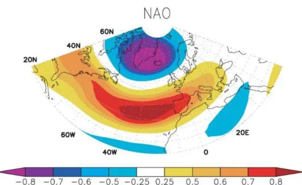
Fig. 2: Spatial pattern of North Atlantic Oscillation (NAO) computed for December–February within the period 1960– 2000 and based on a PCA approach. Figure taken from (Trigo et al., 2008)

Between the the two centers of action, located over quite different latitudes, there is a band where the correlation between the SLP anomaly and the index is weak or equal to zero (Figure 2). During a positive phase of the NAO, the spatial distribution of SLP is characterized by a strong meridional gradient in the North Atlantic as shown in Figure 3 (a). Winds are stronger in the positive phase than in the negative phase (Fig.3 (b)). The meridional gradient tends to diminish during negative phases of the NAO. The shift from one phase to another of the NAO index contributes to the modulation of the trajectories of the depressions in the North Atlantic which causes changes in the transport of heat and humidity and consequently alterations of the temperature and precipitation patterns in a continental scale (Trigo et al., 2004; Hurrel, 2003; IPCC 2007).

Fig. 3: SLP and Wind intensity (arrows) winter climatology for a positive phase(a) and a negative phase (b) of the NAO index for the 1959-2007 period. Figure taken from (Jerez & Trigo, 2013)

In Southwestern Europe winds tend to south-western Iberia from NW during the positive phase and more from the west during the negative phase. Despite the impact of NAO in wind direction, NAO does not change significantly the strength of the wind flow in the Iberian region (Fig. 4). On the contrary, in the northern part of the European coast, such as west of the British islands, a great variability between phases for what concerns the wind intensity has been observed (Figure 4).

Fig. 4: Correlation between winter (October–March) values of wind speed and the corresponding winter NAO index for the period 1960–2000. Figure taken from (Trigo et al. 2008)

1.2.2 East Atlantic Pattern (EA)

In the European side of the North Atlantic, the second most important climate variability mode corresponds to the Atlantic East (EA) Pattern. It has been defined by Barnston & Livezey (1987) as a dipole being centered near 55ºN,20º-35ºW with a strong northwest-southeast gradient over western Europe (the neutral line passing between England or France) and an oppositely signed east-northeast-west-southwest-oriented anomaly band over North Africa or the Mediterranean Sea (Figure 5). The EA pattern has an impact on precipitation and temperature in Europe (Trigo et al., 2008). According to Murphy & Washington (2001), the EA explains the variability pattern of precipitation over Ireland and the UK than the NAO.

Fig. 5: Spatial pattern of East Atlantic (EA) computed for December–February within the period 1960–2000 and based on a PCA approach. Figure taken from (Trigo et al., 2008).

The correlation between EA index and wind intensity over the North Atlantic presents the highest correlation values at lower latitudes than those associated to the NAO pattern (Trigo et al. 2008) (Figure 6).

Fig. 6: Correlation between winter (October–March) values of wind speed and the corresponding winter NAO for the period 1960–2000. Figure taken from (Trigo et al., 2008)

1.2.3 Scandinavian Pattern (SCAND)

The third major mode of climate variability in the North Atlantic/Europe sector is the Scandinavian Pattern (SCAND). It has been defined with a primary center in the Scandinavian/North Sea zone coupled with an oppositely signed weaker center in south-western Europe as shown in Figure 7. The SCAND pattern is, among the climate variability modes used for this work, the one with the most continental expression (Trigo et al. 2008). It has been associated, even if in a less effective way than the NAO and the EA, with anomalies in temperature, precipitation and wind climate in Europe. The positive phase of SCAND is associated with negative temperature and a positive precipitation anomaly in the Iberian region (Trigo et al. 2008).

Fig. 7: Spatial pattern of teleconnection index Scandinavian (SCAND) computed for

December-February within the period 1960–2000 and based on a PCA approach. Figure taken from (Trigo et al., 2008)

Fig. 8: Correlation between winter (October–March) values of wind speed and the corresponding winter SCAND for the period 1960–2000. Figure taken from (Trigo et al., 2008)

The spatial pattern of correlation between the winter SCAND index and wind intensity is shown in Figure 8. The highest correlations have been observed just between the two centers of SCAND. The correlation pattern between the winter values of wind speed and the corresponding SCAND index (Fig.8) is relatively weak and presents the highest values of correlation in the northeastern sector of the Atlantic, between Greenland and Scandinavia (Trigo et al., 2008)

1.2.4 Combination of Modes

Climate variability modes can interact with each other and these interactions modify the structure of their spatial pattern. Comas-Bru & McDermott (2013) studied the modifications of the NAO structure in association with the other two major modes and these modifications in terms of SLP are shown in Figure 9. These authors have evaluated the change of SLP pattern in the NAO standard signature produced by EA and SCAND, taking into account if these modes are in the same (S) or opposite phase (S) of the NAO. Comas-Bry & McDermott (2013) have also concluded that the relative positioning of the EA and the NAO may affect the intensity and the latitude of the westerlies.

Fig. 9: Spatial correlation between SLP and NAO for different combination of indexes for winter (DJF). Each Figure indicates each combination for the same phase (S) and opposite phase (O). Figure taken from (Comas-Bru &

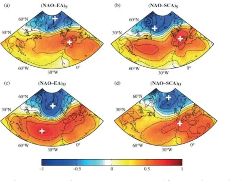
Using a slightly different approach Moore et al. (2011) showed that the EA phase modulates the NAO location and intensity since the northern center of action of the EA is located right along the NAO nodal line. In a similar way, it has been shown by Moore et al., (2013) that the location of the main SCAND center of action imposes mobility on the centers of the NAO dipole. In Figure 10 and 11 we can see how the interaction of the various modes can influence the SLP spatial pattern, as a consequence of these interactions we can observe attenuations or amplifications of the anomalies associated with the undisturbed phase of the modes. Comas-Bru & McDermott (2013) have concluded that the relative positioning of the EA and the NAO may affect the intensity and the latitude of the westerlies.

Fig. 10: Impact of the phase of the NAO and EA on the winter (DJF) monthly mean sea level pressure field (mb) over the North Atlantic for the period 1871–2008.. The figures in the middle column represent the leading EOF (i.e.,

the NAO), while those in the middle row represent the EA pattern. The corner figures represent the linear combinations of these two modes. Figure taken from (Moore et al., 2013)

Fig. 11: As in Fig. 19, but for the SCAND pattern. Figure taken from (Moore et al., 2013)

1.3 Impact on Wave Climate

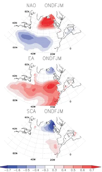
Several published works suggest the hypothesis that teleconnections have an impact on wave climate in the North Atlantic (Dodet et al., 2010; (Trigo et al., 2008). According to these authors, the inter-annual variability of climate modes implies a corresponding variability on wave parameters. In Trigo et al. (2008) the highest correlations (>0.7) of NAO and significant wave height (Hs) were found in northern latitudes between the British Islands and Greenland, a more coherent spatial distribution has been found for EA-Hs correlations with still high (~0.7) maximum values but at lower latitudes than with the NAO. An opposite dipolar pattern has been found for the SCAND-Hs where negative correlations were at higher latitudes than the positive (even if weak) correlations at lowers latitudes.

Fig. 12: Correlation between winter (October-March) values of significant wave height and the corresponding winter NAO (top), EA (middle), and SCAND (bottom) indexes for the period 1970-2000. Figure taken from (Trigo et al.,

2008)

The location of maximum correlation values for the NAO and the EA indexes and the Hs fields were usually located at the east of the corresponding maximum values obtained for the wind pattern; this is due to the fact that Hs is not only dependent on the local wind activity, but also on the swell propagating from more distant storms (Trigo et al., 2008). Also in Dodet et al. (2010) the results obtained show the strong link between the ocean and atmospheric climate dynamics, since inter-annual and long-term variability of significant wave height, peak wave period and mean wave direction were found to be significantly related to the NAO index. In order to explain the correlations in Dodet et al (2010) extreme NAO values were selected. In the case of NAO- (winter 1969/70) low gradients and low mean winds were observed, while in the case of NAO+ (winter of 1988/89) high gradients and strong mean winds produced bigger wave conditions (Fig 13.)

Fig. 13: Winter-mean SLP, winter-mean wind velocity over the North Atlantic Ocean and winter-mean wave spectra at P1 (12.5W; 55.0N) and P3 (12.5W; 35.0N) for the case ‘‘NAO-” in winter 1969 (A–D, respectively) and for the

case ‘‘NAO+” in winter 1989 (E–H, respectively). Figure taken from (Dodet et al., 2010)

1.4 Wind Generated Waves Theory

There are several distinct mechanisms able to generate a gravity wave that propagates across the ocean; nevertheless, the majority of the waves we observe on the ocean surface have been generated by the wind activity over the open sea. The factors that influence the formation and the evolution of waves in deep water are essentially the following three: wind speed, wind duration in time, and fetch, namely the length of the area of ocean surface over which the wind blows with a constant direction.

One candidate model for the initial generation of waves is the instability of the water surface layer in which the wind generates a current. Two fluids with different speeds, such as water and air, will generate perturbations at their interface if speeds and densities differ enough (Lamb, 1932; Holthuijsen, 2007). Another candidate model is the one suggested by (Phillips 1957) in which waves are generated by resonance between propagating wind-induced pressure waves at the water surface. Once initial water waves are finally generated Miles (1957) found that these waves modify the airflow and consequently the wind-induced pressure in a way that enhances their growth.

Phillips‟ theory for a constant wind estimates that the transfer of energy from wind to waves

S





)



,

(

f

S







where f is the frequency, θ the direction and the U_wind the wind intensity vector.

Most of the operational models ignore this mechanism because in reality, small waves are always present to trigger wave growth. Normally initial small waves are just imposed in the model. The growth of the waves, once the first initial small perturbations are created, is described by Miles (1957) who found that the air pressure at the water surface reaches a maximum on the side of the wave exposed to the wind and a minimum on the side protected from the wind by the wave crest, implying that the wind pushes the water surface up and down right when it is moving respectively up and down, as shown in Figure 14.

Fig. 14: The wave-induced wind-pressure variation over a propagating harmonic wave. Figure taken from (Holthuijsen, 2007)

This coupling transfers energy from the atmosphere to the waves, and since it is dependent on the amplitude of the waves it increases its effectiveness as the wave grows in a positive-feedback mechanism:

)

,

(

)

,

(

f





E

f



S













where  is a coefficient that depends on the speed and direction of the wind and the wave,

U

1.5 Wave parameters definition

The wave parameters used to define the wave climate in this work are the Significant Wave Height (Hs) and the Peak Period (Tp).

The Significant Wave Height is defined as the average of one third of the highest waves in a measured wave record, and was intended to mathematically express the wave height estimated by a "trained observer" (Wilson et al., 2002).

The probability density function p(H) for the wave height is given by Rayleigh distribution: ) ( 2 2 2

2

)

(

e

H

H

H

p



where

H

The distribution graph is shown in figure 15. The probability of measuring a wave higher than Hs is indicated as the shadowed area in the graph (

H

H

This probability is given by:

133 . 0 ) ( 2.02 ) 42 . 1 ( ) ( 2 2 2 2         e e e H H p rms rms rms S H H H H S (4)

which means that there is a probability of 13.3% of measuring a wave higher than Hs (Young, 1999).

Fig. 15: Density probability function p(H) for wave height defined by the Rayleigh distribution (eq. 3) Significant wave height Hs is indicated.Figure taken from Young (1999)

The peak wave period (Tp) is defined as the wave period associated with the most energetic waves in the total wave spectrum at a specific point. Wave regimes that are dominated by wind waves tend to have smaller peak wave periods, and regimes that are dominated by swell tend to have larger peak wave periods (NOAA-TAFB). Because the average period is considered to be less statistically stable, and because the higher waves are the most important, it is best to use the peak period as a representative wave period for a spectrum of waves (Sorensen, 1993).

2 Data Sets and Methodology

2.1 Wave data source and location

In an ideal world long-term series of buoy data would be readily available, with no gaps and missing values, however, this is rarely the case. Buoy data may be the wave data source analogically closest to reality, but they often present some limitations in data continuity while satellite altimeter data has only been available since the late eighties (Dodet et al., (2010). Therefore, several authors have employed a spectral wave model in order to guarantee consistency in terms of data continuity and time. In this work, wave data have been produced by a regional wave model over the North-East Atlantic Ocean implemented by Dodet et al., (2010). A wave hindcast simulation was performed with the spectral wave model WAVEWATCH III (Tolman, 2009) forced with the NCEP Reanalysis wind fields (Kalnay et al., 1996), over a spatial grid covering the North Atlantic Ocean, from 80.0° W to 0.0° W in longitude and 0.0° N to 70.0° N in latitude, with a 0.5° resolution. The model was validated by Dodet et al., (2010) against buoy data over the available timefor several buoy locations. From this model time series of representative wave parameters in 10 different locations in the North East Atlantic from 1953 to 2009 have been extracted and have been used for this work. Locations considered cover a wide portion of the western European coast, from 50ºN to 35ºN as illustrated in Figure 1.

2.2 Climate modes indexes

Climate modes data have been taken from the CPC website for the same time interval of the wave data, but with a monthly temporal resolution. The indexes have been calculated using the PCA method applied to the geopotential height field at 500hPa. A winter mean of each mode has been calculated and the indexes where then normalized.

The phase of each mode has been determined by the value of the respective normalized index as it follows:

Positive phase: Index ≥ 0.5

Neutral phase: - 0.5 < Index < 0.5 Neutral phase: Index ≤ -0.5

In frequency of occurrence of winter months (December, January, February and March) for each phase of the analyzed modes for the period 1953-2009, resulting in 224 total winter months analyzed. This is important in order to understand the relative frequency of occurrence of the phases of each mode (also shown in percentage).

Table 1. Number of winter months for negative, neutral and positive phase for NAO, EA and SCAND and the relative percentage of occurrence for the period 1953-2009.

Negative Phase Neutral Phase Positive Phase Total NAO 67 (30%) 77 (34%) 80 (36%) 224 (100%) EA 93 (42%) 72 (32%) 59 (26%) SCAND 61 (27%) 90 (40%) 73 (33%)

As previously mentioned, climate variability modes can interact with each other. Thus it is also important to study the impact of different possible combinations of phases. Excluding the combination of neutral phases, 12 combinations have been obtained as shown in Table 2.

Table 2. Combination of modes: the second column shows which phases are combined indicating also if they are in the same phase or in opposition of phase. Third column shows the number of months in which that particular combination has been observed. The fourth column shows the relative frequency of occurrence. The fifth column shows the total number of months analyzed for every combination. Climate variability modes Combination of modes Nº of monhts Frequency Total NAO & EA S

EA

NAO

)

(

EA

NAO

)

(

EA

NAO

)

(

EA

NAO

)

(

SCAND

NAO

)

(

SCAND

NAO

)

(

SCAND

NAO

)

(

SCAND

NAO

)

(

SCAND

EA

)

(

SCAND

EA

)

(

SCAND

EA

)

(

SCAND

EA

)

(

2.3 Data Analysis

Wave data with a 6 hrs time step every day from 1st _{January 1953 to 31}st

December 2009 with no interruptions or missing data. The parameters used for this analysis are Significant Wave Height (Hs) and Peak Period (Tp). Winter averages of the wave parameters for winter (n) have been considered from December (n-1) to March (n). The focus of the analysis has been concentrated on winter values because the climate modes in analysis have a greater expression in winter (Barnston & Livezey, 1987). Furthermore, various authors (Bacon and Carter, 1993; Bauer, 2001; Wang and Swail, 2001; Woolf et al., 2002; Dodet et al., 2010) have shown that wave height climate is better correlated with the winter NAO index than the monthly NAO index.

The normalization used for wave parameters and climate modes is the standard score that represents the number of standard deviations a variable is above (or below) its mean:

 ) ( _mean normalized x x x   (5)

Temporal correlation (R), computed through the Pearson correlation coefficient, was employed to measure the strength of the relationship between the large-scale circulation indexes and the wave parameters.

The significance of the variations in the distributions of wave parameters was evaluated using the Kolmogorov-Smirnov test.

2.4 Multiple Linear Regression Models (MLRM)

Climate variability modes, as already mentioned, have an impact on many aspects of the climate of one given region. In order to build a diagnostic model based on climate modes, the indexes of each mode can be considered as predictor variables. The inclusion of more than one predictor variable allows for the study of the combined effect of climate modes. The same procedure has been used in (Jerez & Trigo, 2013) by using a multiple linear regression as follows:

)

(

)

(

)

(

)

(

t

C

C

WNAO

t

C

WEA

t

C

WSCAND

t

X









where the coefficients WNAO, WEA and WSCAND represent the predictor variables, which are the winter indexes, and are multiplied by their respective regression coefficients:

C

C

C

C

The accuracy of these modeled series is then evaluated by an objective comparison with the original ones. To this purpose, two scores have been used: the Pearson correlation coefficient (R) between the original and the modeled series, and the standard deviation ratio (stdr) defined as the ratio between the standard deviation

of the modeled series and the standard deviation of the original series (Jerez & Trigo, 2013). The closer the stdr value is to 1, the better the agreement between the

two series is. Lower (or higher) than 1 values indicate a lower (or higher) standard deviation for the modeled series than for the original ones.

Eventual problems related to over fitting were mitigated by employing the always stringent cross-validation scheme, usually known as the leave-one-out scheme (Wilks, 2006). Of the 56 yr of data vailable, 55 yr are used for construction and 1 for validation. A moving window is applied, such that the first run is performed using data for 1954-2009 for construction and data from 1953 for validation; on the second run data for 1953-2008 are used for construction and data from 2009 for model development, and so on (Trigo & Palutikof, 1999; Sousa et al., 2011).

3 Results and Discussion

After a preliminary assessment on the 10 locations it was decided to focusthe work in a few representative locations. Thus locations 1 and 10, the northernmost and the southernmost locations respectively, were used in the context of the current work. The main reason for this choice is related to the spatial gradient (from north to south) that has been observed in the correlations between climate modes and wave parameters, often resulting in two distinct behaviors in the two locations.

3.1 Climatology

In Table 3 the climatology relative to significant wave height and peak period is shown. Highest values of the mean significant wave height tend to be located in the most exposed locations (1, 5 and 6), while the lowest values are found in relatively protected locations. It‟s interesting to notice that the lowest standard deviation values of significant wave height are found in station 3, 8, 9 and 10 also where the longest peak periods are recorded. As shown in figure 16, the distribution of significant wave height is narrower in location 10 than in location 1 while the peak period has a slightly wider distribution in location 10.

Table 3. Climatology of the locations in study

Location

Number Longitude & Latitude Significant Wave Height [m] Peak period [s]

x̄ σ Max. Value x̄ σ 1 07.5 W; 50.0 N 2.35 1.46 12.37 8.20 1.85 2 05.0 W; 47.5 N 1.24 1.41 12.69 8.28 1.82 3 02.5 W; 45.0 N 1.78 1.10 12.04 8.69 1.89 4 05.0 W; 45.0 N 2.11 1.29 12.45 8.60 2.02 5 07.5 W; 45.0 N 2.34 1.38 12.70 8.52 1.98 6 10.0 W; 45.0 N 2.52 1.46 12.69 8.42 1.92 7 10.0 W; 42.5 N 2.21 1.27 11.63 8.65 1.97 8 10.0 W; 40.0 N 2.03 1.11 13.00 8.73 2.03 9 10.0 W; 37.5 N 1.93 1.00 13.27 8.70 2.07 10 10.0 W; 35.0 N 1.82 0.90 11.23 8.74 2.11

Location 10 tends to receive swells that are smaller (in height) but with longer period than those in location 1 due to its latitude, being far from the mid-latitude storm tracks, while location 1 is more often hitten by storms collecting higher waves but with shorter periods.

Fig. 17: Histogram of significant wave height (left) and peak period (right) for the location 1 (top) and location 10 (bottom).

3.2 Impact of each mode on Significant Wave Height and Peak Period

The impact on wave climate of NAO, EA and SCAND was undertaken by analyzing the Pearson correlation between the normalized inter-annual winter (December to March) averages of Hs and Tp and the corresponding winter normalized indexes. As shown in Figure 18a, positive significant (p<0.10) correlation between NAO and Hs with a value of 0.48 has been found in location 1, the correlation coefficients then decrease steadily going south-west, becoming negative south of 42.5Nº and inverting signal, reaching weak (but significant ) correlations in the two

Fig. 18: Pearson correlation coefficients between winter (December–March) values of significant wave height (left), peak period (right) and the corresponding winter NAO (top), EA (middle) and SCAND (bottom)

for the period 1953–2009 for each location. Dots marked with black circles have statistical significance (p<0.10).

southernmost locations (9 and 10) with a negative maximum value of -0.28 in 10. Significant positive correlations have been found for Tp and NAO in every location with a weak north to south spatial distribution with the highest values in northern latitudes (0.60 in 1) and the lowest values in southern latitudes (0.51 in 10) (Fig. 18b). Likewise, EA and Hs correlations are significant and positive in all locations, decreasing from north to south with a maximum value of 0.63 in 1 and a minimum

Fig. 19: Comparisons between the normalized winter NAO (top), EA (middle), SCAND (bottom) and winter-means of Hs (left) and Tp (right) for location 1. The Pearson correlation coefficient is given for each

plot.

value of 0.46 in 10 (Fig. 18c). As for Tp and EA it was also found widespread significant positive correlations everywhere in the area of study with a higher values in southern locations (0.57 in 10) and lower values in the northern locations with a minimum of 0.41 in 1 (Fig. 18d). Finally correlation values between SCAND and Hs have positive significant correlations in locations 6, 7, 8 and 9 with a maximum value of 0.39 in 10 (Fig. 18e). It is interesting to notice that there is a south to north spatial distribution and the correlations, even though

Fig. 20: Comparisons between the normalized winter NAO (top), EA (middle), SCAND (bottom) and winter-means of Hs (left) and Tp (right) for location 10. The Pearson correlation coefficient is given for each

plot.

not significant, become negative north of 45ºN. No relevant relationship has been found in what regards SCAND and Tp, probably because the longer period waves that could be correlated with positive SCAND are starting to be generated in the southern boundary of our area of observation, right where the best SCAND-Hs correlation has been found (Fig.18 e) and f)). Those waves then propagate southwards outside our network of locations. In figures 19 and 20 the temporal evolution of all the modes and respective wave parameters is shown for location 1 and 10.

The impact of climate modes on wave parameters has also been evaluated taking into account the entire winter distribution of significant wave height and peak period. This is achieved by producing histograms for locations 1 and 10 for each phase of each mode and for each parameter (Figures 21, 22, 23 and 24). All the histograms presented are calculated for December-March Winters. Positive NAO phases are associated in location 1 with a wider distribution of Hs and also with a shift towards higher values, while negative phases result in a narrower distribution. Negative phases of EA are strongly associated with smaller wave conditions while positive phases present significantly larger wave conditions. No significant link was found between SCAND phases and Hs in location 1 (Figure 21).

Fig. 21: Histogram for Significant Wave Height in Location 1. The different phases of the modes are represented by different colors.

Regarding the changing in distribution of peak period in location 1 it is possible to observe similar impacts for both NAO and EA with shorter periods associated with the respective negative phases, and longer periods as a result of positive phases (Figure 22). The impact of NAO and EA on wave period is not as strong as the impact on wave height in location 1 since being at a latitude of 50ºN in this location

Fig. 22: Histogram for Peak period in Location 1. The different phases of the modes are represented by different colors.

the higher waves associated with positive phases of NAO and EA have not yet developed in length but are instead still growing in height. Tp variations appear to be not significantly linked with the SCAND phases. Location 10 sees very weak variations in the distribution of Hs both for NAO and SCAND while it is strongly affected by the EA phases as shown in Figure 23. Smaller waves are associated with negative EA phases while positive phases of EA do not differ significantly from neutral phases. Stronger variations are associated with the wave period: with both NAO and EA negative phases resulting in much smaller periods observed in location 10, while there is no significant influence of the SCAND phases. The unsignificant variation in the distribution of Hs associated with NAO in 10 and the strong and positive correlation for Tp is explainable by the fact that location 10 receives swells from northern latitudes (where the correlation between NAO and Hs is significant and positive); those swells during their travel from north to south have time to separate their spectral components and attenuate their wave height but conserving their long period components. Therefore, at lower latitudes such as in 10, long period but small height waves are therefore associated with positive NAO while shorter wave periods are much more common during negative NAO winters.

Fig. 23: Histogram for Significant Wave Height in Location 10. The different phases of the modes are represented by different colors.

3.3 Combination of modes

It must be stressed that each individual winter months is often characterized by significant values of various circulation indices, i.e. the large-scale pattern of atmospheric circulation is not too similar to any of the analyzed but, instead, to a combination of two modes. Thus, in order to study the interactions between two different phases of each mode histograms of Hs and Tp of the December-March Winters have been plotted for all the possible combinations of phases for the locations 1 and 10 (Figures 25 and 26).

Fig. 25: Histograms of Significant Save Height for Location 1 (left) and Location 10 (right). The histograms are divided by colors, each one of which represents different combination between NAO and EA (top),

The histograms are represented in four different colors, each one representing different combinations between NAO and EA (top), NAO and SCAND (middle), SCAND and EA (bottom). NAO and EA patterns interact in such a way that results in a narrower distribution for location 1, and averaged towards small (<2m) values of Hs when they both are in a negative phase, while higher conditions are associated with positive phases of the two indexes.

Fig. 26: Histograms of Significant Save Period for Location 1 (left) and Location 10 (right). The histograms are divided by colors, each one of which represents different combination between NAO and EA (top), NAO and SCAND (middle), SCAND and EA (bottom). The histograms are calculated for DJFM winters

Winter months characterized by opposite phases of NAO and EA tend to weaken their impact in 1 resulting in no statistically significant difference between the NAO+EA- and NAO-EA+ distributions. Unlike location 1, the opposition of the NAO and EA phases is relevant in 10 where the combination EA+NAO- is associated with significantly higher conditions than NAO+EA-. No statistically significant difference has been found in 10 for the combination EA-NAO in the same phase with respect to Hs values. NAO-SCAND and SCAND-EA combinations show weak and not statistically significant variations of the distribution of Hs associated with a change in the SCAND index since it seems they only respond to the NAO and EA oscillations for both locations 1 and 10. As for the impact of combined modes on Winter Tp distributions in locations 1 and 10 it is possible to observe a major role being played by NAO-EA while they are in the same phase; both in 1 and 10 longer period waves are associated with NAO+EA+, while shorter periods are much more common during negative phases NAO-EA-. As previously seen for Hs, the opposition of phases tends to attenuate their impact on Tp. SCAND influence appears to have almost no impact on Tp in both locations. It is interesting to notice that for NAO-SCAND and EA-SCAND combinations the overall change in the distribution is mostly dependent on the phase of NAO and EA respectively.

3.4 Multiple Linear Regression Models (MRLM)

The combined influence of NAO, EA and SCAND was further evaluated through the use of a multi-linear regression model (MLRM) which includes the three large-scale indexes as predictors. The MLRM (Equation 6) has been calibrated using the inter-annual winter means of Hs and Tp. The corresponding patterns of the MLRM-modeled series and the original series for both parameters are shown in figure 27 for location 1 and in figure 28 for location 10. The Pearson correlation coefficient is shown for each plot. Table 4 summarizes the correlations of each mode with the inter-annual winter mean of Hs and Tp and presents also correlations between the original values and the modeled values for each location in analysis with its standard deviation ratio (stdr).

Table 4. Correlations between each one of the modes inter-annual winter means, the MLRM modeled series and the original inter-annual winter means of Hs and Tp for each location. The standard deviation ratio between the modeled and the original series is also given. The underlined values are statistically significant (p<0.10). Location Number Longitude & Latitude NAO EA SCAND MLRM stdr Hs Tp Hs Tp Hs Tp Hs Tp Hs Tp 1 07.5 W; 50.0 N 0.48 0.60 0.63 0.41 -0.13 -0.16 0.71 0.65 0.74 0.68 2 05.0 W; 47.5 N 0.38 0.59 0.61 0.35 -0.04 -0.18 0.64 0.60 0.67 0.64 3 02.5 W; 45.0 N 0.36 0.51 0.58 0.38 0.04 -0.18 0.61 0.53 0.64 0.59 4 05.0 W; 45.0 N 0.34 0.58 0.57 0.36 0.07 -0.18 0.58 0.59 0.62 0.64 5 07.5 W; 45.0 N 0.24 0.57 0.58 0.38 -0.16 -0.16 0.56 0.60 0.58 0.64 6 10.0 W; 45.0 N 0.15 0.57 0.38 0.38 0.16 -0.16 0.58 0.60 0.60 0.64 7 10.0 W; 42.5 N -0.01 0.62 0.57 0.38 0.28 -0.21 0.59 0.65 0.64 0.68 8 10.0 W; 40.0 N -0.14 0.63 0.53 0.44 0.35 -0.21 0.59 0.69 0.64 0.72 9 10.0 W; 37.5 N -0.24 0.57 0.49 0.52 0.38 -0.17 0.57 0.69 0.62 0.72 10 10.0 W; 35.0 N -0.28 0.51 0.46 0.57 0.39 -0.14 0.58 0.69 0.65 0.72

The agreement between the MLRM modeled series and the original series of Hs and Tp is high and statistically significant in all cases with a maximum correlation of 0.71 found for Hs in location 1. The stdr is also well sustained (above 0.5) in all cases with a maximum value of 0.74 for Hs in 1.

Fig. 27: Comparison between the observed Significant Wave Height (top), Peak Period (bottom) and the same parameters modeled using the modes’ indexes as predictor variables for location 1. The

Pearson correlation coefficient is given for each plot.

Fig. 28: Comparison between the observed Significant Wave Height (top), Peak Period (bottom) and the same parameters modeled using the modes indexes as predictor variables for location 10.

It is interesting to notice that the highest correlation found in location 1 for the modeled Hs is obtained using only the NAO and the EA indexes as predictor variables in the MLRM, unlike location 10 that includes all the climate modes in the construction of the MLRM modeled series. All modeled series for Tp only include the NAO and the EA as predictors.

4 Conclusions

This work evaluated the impact of three major climate variability modes in the Euro-Atlantic region (NAO, EA and SCAND) on the wave climate along the European western coast. First, an assessment of the correlation values between normalized inter-annual winter (December-March) means of Hs and Tp and their relative inter-annual means of winter NAO, EA and SCAND has been done in 10 representative locations on the western European coast. The results show that the inter-annual variability of winter wave characteristics can be associated, to a large extent, with the indexes of NAO and EA. The impact of SCAND on Hs has only been found statistically significant south of 42.5ºN with its correlation coefficient increasing southward. This spatial distribution of SCAND suggests that stronger correlations for both Hs and Tp could be found widening the observation to southern latitudes.

The analysis of the winter distributions of Hs and Tp for different phases of each single mode confirmed the major impact of NAO and EA on the winter wave climate of the European coast. However, it can be misleading to evaluate the impact of these circulation modes individually, as they often reveal large values simultaneously.

Winter distributions of Hs and Tp showed statistically significant variability for different combinations of NAO and EA phases. Two clusters of opposite behavior have been found between the northernmost (1) and southernmost (10) location. The results obtained in 1 showed that when NAO and EA are in the same positive phase one can expect higher values of both Ts and Hs, while the same negative phases for both NAO and EA result in much smaller and weaker conditions. On the contrary, when both indexes are in opposition of phases they tend to annihilate

their effects resulting in values for the distributions of Hs and Ts not significantly different from their winter climatology.

Less evident but still statistically significant variations have been found in location 10 for the Hs distribution but for reversed combinations. Opposition of phases results in bigger conditions in the NAO-EA+ case while significantly smaller conditions are associated with the NAO+EA- combination. When EA and NAO are in the same phase they tend to balance their effects resulting in a narrower and more centered towards average values distribution. The Tp distribution in 10 has been found to be associated by the variation of Tp and Hs in 1. This is due to the fact that the high period waves that reach location 10 are generated by storms in the same latitude of those striking 1 (50ºN) even if much more to the west. This fact suggests that the extension of the impact of the combined NAO and EA on wave climate is extended to a wider portion of the North Atlantic. Overall SCAND influence on Ts and Tp winter distributions has not been found significant anywhere in the network of locations in study.

The MLRM modeled series of Hs and Tp showed high correlations with the original ones in all the locations with a maximum of 0.71 in 1. The lack of statistical significance of the SCAND index correlations with Hs values in the northernmost locations, and with Tp values in all the locations, resulted in the exclusion of that mode as a predictor variable in MLRM modeled series for those locations, confirming once again the leading impact of the NAO and EA modes.

The strong variability associated with the combination of phases and the overall good agreement obtained by the MLRM reconstructed series show that the impact of climate variability modes, especially NAO and EA, on wave parameters on the European coast is stronger when the combined action of the modes is taken into consideration.