arXiv:1412.7086v2 [hep-ex] 15 Jul 2015
EUROPEAN ORGANISATION FOR NUCLEAR RESEARCH (CERN)
CERN-PH-EP-2014-227
Submitted to: Eur. Phys. J. C
Identification and energy calibration of hadronically decaying
tau leptons with the ATLAS experiment in
pp
collisions at
√s
=8 TeV
The ATLAS Collaboration
Abstract
This paper describes the trigger and offline reconstruction, identification and energy calibration
algorithms for hadronic decays of tau leptons employed for the data collected from
pp
collisions in
2012 with the ATLAS detector at the LHC center-of-mass energy
√
s
= 8 TeV. The performance of
these algorithms is measured in most cases with
Z
decays to tau leptons using the full 2012 dataset,
corresponding to an integrated luminosity of 20.3 fb
−1. An uncertainty on the offline reconstructed
tau energy scale of
2 − 4
%, depending on transverse energy and pseudorapidity, is achieved using
two independent methods. The offline tau identification efficiency is measured with a precision of
2.5% for hadronically decaying tau leptons with one associated track, and of 4% for the case of three
associated tracks, inclusive in pseudorapidity and for a visible transverse energy greater than
20
GeV.
For hadronic tau lepton decays selected by offline algorithms, the tau trigger identification efficiency
is measured with a precision of
2 − 8
%, depending on the transverse energy. The performance of the
tau algorithms, both offline and at the trigger level, is found to be stable with respect to the number of
concurrent proton-proton interactions and has supported a variety of physics results using hadronically
decaying tau leptons at ATLAS.
c
2015 CERN for the benefit of the ATLAS Collaboration.
Noname manuscript No. (will be inserted by the editor)
Identification and energy calibration of hadronically decaying
tau leptons with the ATLAS experiment in
pp collisions at
√s=8 TeV
The ATLAS Collaboration
Received: date / Accepted: date
Abstract This paper describes the trigger and offline reconstruction, identification and energy calibration al-gorithms for hadronic decays of tau leptons employed for the data collected from pp collisions in 2012 with the ATLAS detector at the LHC center-of-mass energy √
s = 8 TeV. The performance of these algorithms is measured in most cases with Z decays to tau leptons using the full 2012 dataset, corresponding to an
inte-grated luminosity of 20.3 fb−1. An uncertainty on the
offline reconstructed tau energy scale of 2−4%, depend-ing on transverse energy and pseudorapidity, is achieved using two independent methods. The offline tau identifi-cation efficiency is measured with a precision of 2.5% for hadronically decaying tau leptons with one associated track, and of 4% for the case of three associated tracks, inclusive in pseudorapidity and for a visible transverse energy greater than 20 GeV. For hadronic tau lepton decays selected by offline algorithms, the tau trigger identification efficiency is measured with a precision of 2 − 8%, depending on the transverse energy. The per-formance of the tau algorithms, both offline and at the trigger level, is found to be stable with respect to the number of concurrent proton-proton interactions and has supported a variety of physics results using hadron-ically decaying tau leptons at ATLAS.
Keywords LHC · ATLAS · tau 1 Introduction
With a mass of 1.777 GeV and a proper decay length of 87 µm [1], tau leptons decay either leptonically (τ → ℓνℓντ, ℓ = e, µ) or hadronically (τ → hadrons ντ,
denoted τhad) and do so typically before reaching active
regions of the ATLAS detector. They can thus only be identified via their decay products. In this paper, only hadronic tau lepton decays are considered. The hadronic tau lepton decays represent 65% of all possi-ble decay modes [1]. In these, the hadronic decay prod-ucts are one or three charged pions in 72% and 22% of all cases, respectively. Charged kaons are present in the majority of the remaining hadronic decays. In 78% of all hadronic decays, up to one associated neutral pion is also produced. The neutral and charged hadrons stem-ming from the tau lepton decay make up the visible decay products of the tau lepton, and are in the follow-ing referred to as τhad-vis.
The main background to hadronic tau lepton de-cays is from jets of energetic hadrons produced via the fragmentation of quarks and gluons. This background is already present at trigger level (also referred to as
onlinein the following). Other important backgrounds
are electrons and, to a lesser degree, muons, which can mimic the signature of tau lepton decays with one charged hadron. In the context of both the trigger and the offline event reconstruction (shortened to simply
offlinein the following), discriminating variables based
on the narrow shower shape, the distinct number of charged particle tracks and the displaced tau lepton decay vertex are used.
Final states with hadronically decaying tau lep-tons are an important part of the ATLAS physics program. Examples are measurements of Standard Model processes [2,3,4,5,6], Higgs boson searches [7], searches for new physics such as Higgs bosons in mod-els with extended Higgs sectors [8,9,10], supersymme-try (SUSY) [12,13,11], heavy gauge bosons [14] and leptoquarks [15]. This places strong requirements on
the τhad-vis identification algorithms (in the following,
performance over at least two orders of magnitude in transverse momentum with respect to the beam axis
(pT) of τhad-vis, from about 15 GeV (decays of W and
Z bosons or scalar tau leptons) to a few hundred GeV (SUSY Higgs boson searches) and up to beyond 1 TeV
(Z′ searches). At the same time, an excellent energy
resolution and small energy scale uncertainty are par-ticularly important where resonances decaying to tau leptons need to be separated (e.g. Z → ττ from H → ττ mass peaks). The triggering for final states which rely exclusively on tau triggers is particularly challenging, e.g. H → ττ where both tau leptons decay hadroni-cally. At the trigger level, in addition to the challenges of offline tau identification, bandwidth and time con-straints need to be satisfied and the trigger identifica-tion is based on an incomplete reconstrucidentifica-tion of the event. The ATLAS trigger system, together with the detector and the simulation samples used for the stud-ies presented, are briefly described in Sect. 2.
The ATLAS offline tau identification uses various discriminating variables combined in Boosted Decision Trees (BDT) [16,17] to reject jets and electrons. The offline tau energy scale is set by first applying a local hadronic calibration (LC) [18] appropriate for a wide range of objects and then an additional tau-specific correction based on simulation. The online tau iden-tification is implemented in three different steps, as is required by the ATLAS trigger system architecture [19]. The same identification and energy calibration proce-dures as for offline are used in the third level of the trigger, while the first and second trigger levels rely on coarser identification and energy calibration proce-dures. A description of the trigger and offline τhad-vis re-construction and identification algorithms is presented in Sect. 3, and the trigger and offline energy calibration algorithms are discussed in Sect. 5.
The efficiency of the identification and the energy scale are measured in dedicated studies using a Z → ττ-enhanced event sample of collision data recorded by the ATLAS detector [20] at the LHC [21] in 2012 at a centre-of-mass energy of 8 TeV. This is described in Sect. 4 and Sect. 5. Conclusions and outlook are pre-sented in Sect. 6.
2 ATLAS detector and simulation 2.1 The ATLAS detector
The ATLAS detector [20] consists of an inner track-ing system surrounded by a superconducttrack-ing solenoid, electromagnetic (EM) and hadronic (HAD) calorime-ters, and a muon spectrometer (MS). The inner detec-tor (ID) is immersed in a 2 T axial magnetic field, and
consists of pixel and silicon microstrip (SCT) detectors inside a transition radiation tracker (TRT), providing
charged-particle tracking in the region |η| < 2.5.1 The
EM calorimeter uses lead and liquid argon (LAr) as absorber and active material, respectively. In the cen-tral rapidity region, the EM calorimeter is divided in three layers, one of them segmented in thin η strips
for optimal γ/π0 separation, and completed by a
pre-sampler layer for |η| < 1.8. Hadron calorimetry is based on different detector technologies, with scintil-lator tiles (|η| < 1.7) or LAr (1.5 < |η| < 4.9) as ac-tive medium, and with steel, copper, or tungsten as the absorber material. The calorimeters provide coverage within |η| < 4.9. The MS consists of superconducting air-core toroids, a system of trigger chambers covering the range |η| < 2.4, and high-precision tracking cham-bers allowing muon momentum measurements within |η| < 2.7.
Physics objects are identified using their specific de-tector signatures; electrons are reconstructed by match-ing a track from the ID to an energy deposit in the calorimeters [22,23], while muons are reconstructed us-ing tracks from the MS and ID [24]. Jets are
recon-structed using the anti-kt algorithm [25] with a
dis-tance parameter R = 0.4. Three-dimensional clusters of calorimeter cells called TopoClusters [26], calibrated using a local hadronic calibration [18], serve as inputs to the jet algorithm. The missing transverse momentum
(with magnitude Emiss
T ) is computed from the
combina-tion of all reconstructed physics objects and the remain-ing calorimeter energy deposits not included in these objects [27].
The ATLAS trigger system [19] consists of three levels; the first level (L1) is hardware-based while the second (L2) and third (Event Filter, EF) levels are software-based. The combination of L2 and the EF are referred to as the high-level trigger (HLT). The L1 trig-ger identifies regions-of-interest (RoI) using information from the calorimeters and the muon spectrometer. The delay between a beam crossing and the trigger decision (latency) is approximately 2 µs at L1. The L2 system typically takes the RoIs produced by L1 as input and re-fines the quantities used for selection after taking into account the information from all subsystems. The la-tency at L2 is on average 40 ms, but can be as large
1 ATLAS uses a right-handed coordinate system with its
origin at the nominal interaction point (IP) in the centre of the detector and the z-axis along the beam direction. The x-axis points from the IP to the centre of the LHC ring, and the y-axis points upward. Cylindrical coordinates (r, φ) are used in the transverse (x, y) plane, φ being the azimuthal angle around the beam direction. The pseudorapidity is defined in terms of the polar angle θ as η = − ln tan(θ/2). The distance ∆R in the η–φ space is defined as ∆R =p
Identification and energy calibration of hadronically decaying tau leptons in ATLAS at 3
Process Trigger Requirements at EF [GeV]
H±
→τhadν τhad-vis + ETmiss pT(τ ) > 29 E miss T > 50
HSM→τhadτlep, Z →τhadτlep τhad-vis + e pT(τ ) > 20 pT(e) > 18
τhad-vis + µ pT(τ ) > 20 pT(µ) > 15
HSM→τhadτhad τhad-vis + τhad-vis pT(τ1) > 29 pT(τ2) > 20
SUSY(τhadτhad), HSUSY→τhadτhad τhad-vis + τhad-vis pT(τ1) > 38 pT(τ2) > 38
Z’→τhadτhad τhad-vis + τhad-vis pT(τ1) > 100 pT(τ2) > 70
W ’→τhadν τhad-vis pT(τ ) > 115
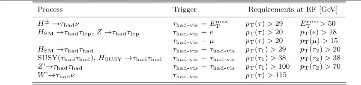
Table 1 Tau triggers with their corresponding kinematic requirements. Examples of physics processes targeted by each trigger are also listed, where τhad and τleprefer to hadronically and leptonically decaying tau leptons, respectively.
as 100 ms at the highest instantaneous luminosities. At the EF level, algorithms similar to those run in the of-fline reconstruction are used to select interesting events with an average latency of about 1 s.
During 2012, the ATLAS detector was operated with a data-taking efficiency greater than 95%. The
highest peak luminosity obtained was 8 · 1033cm−2s−1
at the end of 2012. The observed average number of pile-up interactions (meaning generally soft proton– proton interactions, superimposed on one hard proton– proton interaction) per bunch crossing in 2012 was 20.7. At the end of the data-taking period, the trigger system was routinely working with an average (peak) output rate of 700 Hz (1000 Hz).
2.2 Tau trigger operation
In 2012, a diverse set of tau triggers was implemented, using requirements on different final state configura-tions to maximize the sensitivity to a large range of physics processes. These triggers are listed in Table 1, along with the targeted physics processes and the as-sociated kinematic requirements on the triggered ob-jects. For the double hadronic triggers, in the lowest threshold version (29 and 20 GeV requirement on
trans-verse momentum for the two τhad-vis) two main criteria
are applied: isolation at L12, and full tau
identifica-tion at the HLT. The isolaidentifica-tion requirement is dropped for the intermediate threshold version, and both crite-ria are dropped in favour of a looser (more than 95% efficient), non-isolated trigger for the version with the highest thresholds.
As the typical rejection rates of τhad-vis
identifica-tion algorithms against the dominant multi-jet back-grounds are considerably smaller than those of
elec-tron or muon identification algorithms, τhad-vistriggers
must have considerably higher pT requirements in
or-der to maintain manageable trigger rates. Therefore,
2 A detailed definition of the isolation requirement is
pro-vided in Sect. 3.3.
most analyses using low-pT τhad-visin 2012 depend on
the use of triggers which identify other objects. How-ever, by combining tau trigger requirements with re-quirements on other objects, lower thresholds can be accommodated for the tau trigger objects as well as the other objects.
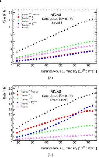
Figure 1 shows the tau trigger rates at L1 and the EF as a function of the instantaneous luminosity dur-ing the 8 TeV LHC operation. The trigger rates do not increase more than linearly with the luminosity, due the robust performance of the trigger algorithms under different pile-up conditions. The only exception is the
τhad-vis+ EmissT trigger, where the extra pile-up
associ-ated with the higher luminosity leads to a degradation
of the resolution of the reconstructed event Emiss
T . At
the highest instantaneous luminosities, the rates are af-fected by deadtime in the readout systems, leading to a general drop in the rates.
2.3 Simulation and event samples
The optimization and measurement of tau performance
requires simulated events. Events with Z/γ∗and W
bo-son production were generated using alpgen [28] in-terfaced to herwig [29] or Pythia6 [30] for fragmen-tation, hadronization and underlying-event (UE) mod-elling. In addition, Z → ττ and W → τν events were generated using Pythia8 [31], and provide a larger sta-tistical sample for the studies. For optimization at high
pT, Z′→ ττ with Z′masses between 250 GeV and 1250
GeV were generated with Pythia8. Top-quark-pair as well as single-top-quark events were generated with
mc@nlo+herwig [32], with the exception of t-channel
single-top production, where AcerMC+Pythia6 [33] was used. W Z and ZZ diboson events were generated with herwig, and W W events with alpgen+herwig. In all samples with τ leptons, except for those simu-lated with Pythia8, Tauola [34] was used to model the τ decays, and Photos [35] was used for soft QED radiative corrections to particle decays.
] -1 s -2 cm 32 Instantaneous Luminosity [10 20 30 40 50 60 70 Rate [kHz] 0 2 4 6 8 10 12 14 had-vis τ + had-vis τ µ + had-vis τ + e had-vis τ miss T + E had-vis τ had-vis τ ATLAS = 8 TeV s Data 2012, Level 1 (a) ] -1 s -2 cm 32 Instantaneous Luminosity [10 20 30 40 50 60 70 Rate [Hz] 0 2 4 6 8 10 12 14 16 18 20 had-vis τ + had-vis τ µ + had-vis τ + e had-vis τ miss T + E had-vis τ had-vis τ ATLAS = 8 TeV s Data 2012, Event Filter (b)
Fig. 1 Tau trigger rates at (a) Level 1 and (b) Event Filter as a function of the instantaneous luminosity for√s = 8 TeV. The triggers shown are described in Table 1, with the τhad-vis
+τhad-vis being the rate for the lowest threshold trigger
re-ported in the table. The rates for the higher threshold triggers are approximately three and five times lower at L1 and HLT, respectively, and are partially included in the rate of the low-est threshold item.
All events were produced using CTEQ6L1 [36]
parton distribution functions (PDFs) except for the
mc@nloevents, which used CT10 PDFs [37]. The UE
simulation was tuned using collision data. Pythia8 events employed the AU2 tune [38], herwig events the AUET2 tune [39], while alpgen+Pythia6 used the Perugia2011C tune [40] and AcerMC+Pythia6 the AUET2B tune [41].
The response of the ATLAS detector was simulated using GEANT4 [42,43] with the hadronic-shower model QGSP BERT [44,45] as baseline. Alternative models (FTFP BERT [46] and QGSP) were used to estimate systematic uncertainties. Simulated events were over-laid with additional minimum-bias events generated with Pythia8 to account for the effect of multiple inter-actions occurring in the same and neighbouring bunch
crossings (called pile-up). Prior to any analysis, the sim-ulated events were reweighted such that the distribution of the number of pile-up interactions matched that in data. The simulated events were reconstructed with the same algorithm chain as used for collision data.
3 Reconstruction and identification of hadronic tau lepton decays
In the following, the τhad-visreconstruction and identifi-cation at online and offline level are described. The trig-ger algorithms were optimized with respect to hadronic tau decays identified by the offline algorithms. This typ-ically leads to online algorithms resembling their offline counterparts as closely as possible with the information available at a given trigger level. To reflect this, the de-tails of the offline reconstruction and identification are described first, and then a discussion of the trigger al-gorithms follows, highlighting the differences between the two implementations.
3.1 Reconstruction
The τhad-vis reconstruction algorithm is seeded by
calorimeter energy deposits which have been recon-structed as individual jets. Such jets are formed
us-ing the anti-ktalgorithm with a distance parameter of
R = 0.4, using calorimeter TopoClusters as inputs. To
seed a τhad-vis candidate, a jet must fulfil the
require-ments of pT> 10 GeV and |η| < 2.5. Events must have
a reconstructed primary vertex with at least three as-sociated tracks. In events with multiple primary vertex candidates, the primary vertex is chosen to be the one
with the highest Σp2
T,tracksvalue. In events with
multi-ple simultaneous interactions, the chosen primary ver-tex does not always correspond to the verver-tex at which the tau lepton is produced. To reduce the effects of pile-up and increase reconstruction efficiency, the tau lepton production vertex is identified, amongst the previously reconstructed primary vertex candidates in the event.
The tau vertex (TV) association algorithm uses as
input all tau candidate tracks which have pT> 1 GeV,
satisfy quality criteria based on the number of hits in the ID, and are in the region ∆R < 0.2 around the jet seed direction; no impact parameter requirements
are applied. The pT of these tracks is summed and the
primary vertex candidate to which the largest fraction
of the pT sum is matched to is chosen as the TV [47].
This vertex is used in the following to determine
the τhad-vis direction, to associate tracks and to build
the coordinate system in which identification variables are calculated. In Z → ττ events, the TV coincides
Identification and energy calibration of hadronically decaying tau leptons in ATLAS at 5
with the highest Σp2
T,tracks vertex (for the pile-up
pro-file observed during 2012) roughly 90% of the time. For
physics analyses which require higher-pT objects, the
two coincide in more than 99% of all cases.
The τhad-vis three-momentum is calculated by first
computing η and φ of the barycentre of the TopoClus-ters of the jet seed, calibrated at the LC scale, as-suming a mass of zero for each constituent. The four-momenta of all clusters in the region ∆R < 0.2 around the barycentre are recalculated using the TV coordinate system and summed, resulting in the momentum
mag-nitude pLCand a τ
had-visdirection. The τhad-vismass is
defined to be zero.
Tracks are associated with the τhad-vis if they are
in the core region ∆R < 0.2 around the τhad-vis
direc-tion and satisfy the following criteria: pT> 1 GeV, at
least two associated hits in the pixel layers of the inner detector, and at least seven hits in total in the pixel and the SCT layers. Furthermore, requirements are im-posed on the distance of closest approach of the track
to the TV in the transverse plane, |d0| < 1.0 mm, and
longitudinally, |z0sin θ| < 1.5 mm. When classifying a
τhad-vis candidate as a function of its number of
asso-ciated tracks, the selection listed above is used. Tracks in the isolation region 0.2 < ∆R < 0.4 are used for the calculation of identification variables and are required to satisfy the same selection criteria.
A π0 reconstruction algorithm was also developed.
In a first step, the algorithm measures the number of re-constructed neutral pions (zero, one or two), Nπ0, in the core region, by looking at global tau features measured using strip layer and calorimeter quantities, and track momenta, combined in BDT algorithms. In a second step, the algorithm combines the kinematic
informa-tion of tracks and of clusters likely stemming from π0
decays. A candidate π0decay is composed of up to two
clusters among those found in the core region of τhad-vis
candidates. Cluster properties are used to assign a π0
likeness score to each cluster found in the core region, after subtraction of the contributions from pile-up, the underlying event and electronic noise (estimated in the isolation region). Only those clusters with the highest scores are used, together with the reconstructed tracks
in the core region of the τhad-vis candidate, to define
the input variables for tau identification described in the next section.
3.2 Discrimination against jets
The reconstruction of τhad-viscandidates provides very
little rejection against the jet background. Jets in which
the dominant particle3 is a quark or a gluon are
re-ferred to as quark-like and gluon-like jets, respectively. Quark-like jets are on average more collimated and have
fewer tracks and thus the discrimination from τhad-visis
less effective than for gluon-like jets. Rejection against jets is provided in a separate identification step us-ing discriminatus-ing variables based on the tracks and TopoClusters (and cells linked to them) found in the
core or isolation region around the τhad-vis candidate
direction. The calorimeter measurements provide infor-mation about the longitudinal and lateral shower shape
and the π0content of tau hadronic decays.
The full list of discriminating variables used for tau identification is given below and is summarized in Ta-ble 2.
Central energy fraction (fcent): Fraction of
trans-verse energy deposited in the region ∆R < 0.1 with respect to all energy deposited in the region
∆R < 0.2 around the τhad-vis candidate calculated
by summing the energy deposited in all cells belong-ing to TopoClusters with a barycentre in this re-gion, calibrated at the EM energy scale. Biases due to pile-up contributions are removed using a correc-tion based on the number of reconstructed primary vertices in the event.
Leading track momentum fraction (ftrack): The
transverse momentum of the highest-pT charged
particle in the core region of the τhad-vis candidate,
divided by the transverse energy sum, calibrated at the EM energy scale, deposited in all cells belonging to TopoClusters in the core region. A correction depending on the number of reconstructed primary vertices in the event is applied to this fraction, making the resulting variable pile-up independent.
Track radius (Rtrack): pT-weighted distance of the
associated tracks to the τhad-vis direction, using all
tracks in the core and isolation regions.
Leading track IP significance (Sleadtrack):
Transverse impact parameter of the highest-pT
track in the core region, calculated with respect to the TV, divided by its estimated uncertainty.
Number of tracks in the isolation region (Niso
track):
Number of tracks associated with the τhad-visin the
region 0.2 < ∆R < 0.4.
Maximum ∆R (∆RMax): The maximum ∆R
be-tween a track associated with the τhad-viscandidate
and the τhad-vis direction. Only tracks in the core
region are considered.
Transverse flight path significance (STflight): The
decay length of the secondary vertex (vertex
recon-3 This is often interpreted as the parton initiating the jet
or the highest-pTparton within a jet; however, none of these
structed from the tracks associated with the core
region of the τhad-vis candidate) in the transverse
plane, calculated with respect to the TV, divided by its estimated uncertainty. It is defined only for
multi-track τhad-viscandidates.
Track mass (mtrack): Invariant mass calculated
from the sum of the four-momentum of all tracks in the core and isolation regions, assuming a pion mass for each track.
Track-plus-π0-system mass (m
π0+track):
Invariant mass of the system composed of the
tracks and π0mesons in the core region.
Number of π0 mesons (N
π0): Number of π
0 mesons reconstructed in the core region.
Ratio of track-plus-π0-system p
T (p
π0+track
T /pT):
Ratio of the pT estimated using the track + π0
information to the calorimeter-only measurement.
Variable Offline Trigger
1-track 3-track 1-track 3-track
fcent • • • • ftrack • • • • Rtrack • • • • Sleadtrack • • Niso track • • ∆RMax • • SflightT • • mtrack • • mπ0+track • • Nπ0 • • pπ0+track T /pT • •
Table 2 Discriminating variables used as input to the tau identification algorithm at offline reconstruction and at trig-ger level, for 1-track and 3-track candidates. The bullets in-dicate whether a particular variable is used for a given selec-tion. The π0-reconstruction-based variables, m
π0+track, Nπ0,
pπ0+track
T /pTare not used in the trigger.
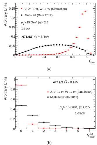
The distributions of some of the important discrim-inating variables listed in Table 2 are shown in Figs. 2 and 3.
Separate BDT algorithms are trained for 1-track
and 3-track τhad-visdecays using a combination of
sim-ulated tau leptons in Z, W and Z′ decays. For the jet
background, large collision data samples collected by jet triggers, referred from now on as the multi-jet data samples, are used. For the signal, only reconstructed
τhad-viscandidates matched to the true (i.e.,
generator-level) visible hadronic tau decay products in the region around ∆R < 0.2 with ptrue
T,vis> 10 GeV and |ηtruevis | < 2.3 are used. In the following, the signal efficiency is de-fined as the fraction of true visible hadronic tau decays
cent f 0 0.2 0.4 0.6 0.8 1 Arbitrary Units 0 0.05 0.1 0.15 0.2 0.25 Z, Z’ →ττ, W →τν (Simulation) Multi-Jet (Data 2012) = 8 TeV s ATLAS 1-track |< 2.5 η > 15 GeV, | T p (a) track iso N 0 1 2 3 4 5 6 Arbitrary Units 0 0.2 0.4 0.6 0.8 1 (Simulation) ν τ → , W τ τ → Z, Z’ Multi-Jet (Data 2012) 1-track = 8 TeV s ATLAS |< 2.5 η > 15 GeV, | T p (b)
Fig. 2 Signal and background distribution for the 1-track τhad-vis decay offline tau identification variables (a) fcent
and (b) Niso
track. For signal distributions, 1-track τhad-vis
de-cays are matched to true generator-level τhad-visin simulated
events, while the multi-jet events are obtained from the data.
with n charged decay products, which are reconstructed with n associated tracks and satisfy tau identification criteria. The background efficiency is the fraction of
re-constructed τhad-viscandidates with n associated tracks
which satisfy tau identification criteria, measured in a background-dominated sample.
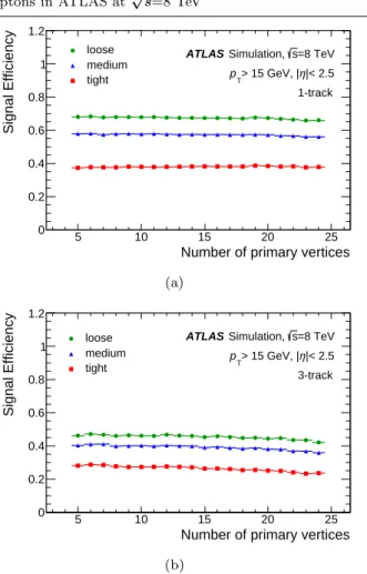
Three working points, labelled tight, medium and loose, are provided, corresponding to different tau iden-tification efficiency values. Their signal efficiency values (defined with respect to 1-track or 3-track reconstructed
τhad-viscandidates matched to true τhad-vis) can be seen
in Fig. 4. The requirements on the BDT score are cho-sen such that the resulting efficiency is independent of
the true τhad-vis pT. Due to the choice of input
vari-ables, the tau identification also shows stability with respect to the pile-up conditions as shown in Fig. 4. The performance of the tau identification algorithm in terms of the inverse background efficiency versus the signal efficiency is shown in Fig. 5. At low transverse
Identification and energy calibration of hadronically decaying tau leptons in ATLAS at 7 track R 0 0.05 0.1 0.15 0.2 0.25 0.3 0.35 Arbitrary Units 0 0.05 0.1 0.15 0.2 0.25 0.3 0.35 0.4 (Simulation) ν τ → , W τ τ → Z, Z’ Multi-Jet (Data 2012) 3-track = 8 TeV s ATLAS |< 2.5 η > 15 GeV, | T p (a) [GeV] +track 0 π m 0.5 1 1.5 2 2.5 3 3.5 4 4.5 5 Arbitrary Units 0 0.02 0.04 0.06 0.08 0.1 0.12 0.14 0.16 (Simulation) ν τ → , W τ τ → Z, Z’ Multi-Jet (Data 2012) 3-track = 8 TeV s ATLAS |< 2.5 η > 15 GeV, | T p (b)
Fig. 3 Signal and background distribution for the 3-track τhad-vis decay offline tau identification variables (a) Rtrack
and (b) mπ0+track. For signal distributions, 3-track τhad-vis
decays are matched to true generator-level τhad-vis in
sim-ulated events, while the multi-jet events are obtained from data.
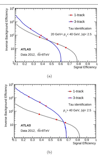
momentum of the τhad-vis candidates, 40% signal
ef-ficiency for an inverse background efef-ficiency of 60 is achieved. The signal efficiency saturation point, visible in these curves, stems from the reconstruction efficiency
for a true τhad-viswith one or three charged decay
prod-ucts to be reconstructed as a 1-track or 3-track τhad-vis
candidate. The main sources of inefficiency are track reconstruction efficiency due to hadronic interactions and migration of the number of reconstructed tracks due to conversions or underlying-event tracks being er-roneously associated with the tau candidate.
3.3 Tau trigger implementation
The tau reconstruction at the trigger level has differ-ences with respect to its offline counterpart due to the technical limitations of the trigger system. At L1, no in-ner detector track reconstruction is available, and the
Number of primary vertices
5 10 15 20 25 Signal Efficiency 0 0.2 0.4 0.6 0.8 1 1.2 loose medium tight pT> 15 GeV, |η|< 2.5 1-track =8 TeV s Simulation, ATLAS (a)
Number of primary vertices
5 10 15 20 25 Signal Efficiency 0 0.2 0.4 0.6 0.8 1 1.2 loose medium tight |< 2.5 η > 15 GeV, | T p 3-track =8 TeV s Simulation, ATLAS (b)
Fig. 4 Offline tau identification efficiency dependence on the number of reconstructed interaction vertices, for (a) 1-track and (b) 3-track τhad-visdecays matched to true τhad-vis(with
corresponding number of charged decay products) from SM and exotic processes in simulated data. Three working points, corresponding to different tau identification efficiency values, are shown.
full calorimeter granularity cannot be accessed. Latency limits at L2 prevent the use of the TopoCluster algo-rithm, and only allow the candidate reconstruction to be performed within the given RoI. At the EF, the same tau reconstruction and identification methods as offline
are used, except for the π0 reconstruction. In this
sec-tion, the details of the tau trigger reconstruction algo-rithm are described.
Level 1 At L1, the τhad-vis candidates are selected
us-ing calorimeter energy deposits. Two calorimeter re-gions are defined by the tau trigger for each candi-date, using trigger towers in both the EM and HAD calorimeters: the core region, and an isolation region around this core. The trigger towers have a granularity of ∆η × ∆φ = 0.1 × 0.1 with a coverage of |η| < 2.5. The core region is defined as a square of 2 × 2 trigger towers, corresponding to 0.2 × 0.2 in ∆η × ∆φ space.
Signal Efficiency
0.1 0.2 0.3 0.4 0.5 0.6 0.7 0.8 0.9 1
Inverse Background Efficiency
1 10 2 10 3 10 4 10 |< 2.5 η < 40 GeV, | T p 20 GeV< ATLAS =8TeV s Data 2012, Tau identification 1-track 3-track (a) Signal Efficiency 0.1 0.2 0.3 0.4 0.5 0.6 0.7 0.8 0.9 1
Inverse Background Efficiency
1 10 2 10 3 10 4 10 |< 2.5 η > 40 GeV, | T p ATLAS =8TeV s Data 2012, Tau identification 1-track 3-track (b)
Fig. 5 Inverse background efficiency versus signal efficiency for the offline tau identification, for (a) a low-pT and (b) a
high-pTτhad-vis range. Simulation samples for signal include
a mixture of Z, W and Z′
production processes, while data from multi-jet events is used for background. The red markers correspond to the three working points mentioned in the text. The signal efficiency shown corresponds to the total efficiency of τhad-vis decays to be reconstructed as 1-track or 3-track
and pass tau identification selection.
The ET of a τhad-vis candidate at L1 is taken as the
sum of the transverse energy in the two most energetic neighbouring central towers in the EM calorimeter core region, and in the 2 × 2 towers in the HAD calorimeter,
all calibrated at the EM scale. For each τhad-vis
candi-date, the EM isolation is calculated as the transverse energy deposited in the annulus between 0.2 × 0.2 and 0.4 × 0.4 in the EM calorimeter.
To suppress background events and thus reduce trig-ger rates, an EM isolation energy of less than 4 GeV is
required for the lowest ET threshold at L1. Hardware
limitations prevent the use of an ET-dependent
selec-tion. This requirement reduces the efficiency of τhad-vis
events by less than 2% over most of the kinematic range.
Larger efficiency losses occur for τhad-vis events at high
ETvalues; those are recovered through the use of
trig-gers with higher ET thresholds but without any
isola-tion requirements.
The energy resolution at L1 is significantly lower than at the offline level. This is due to the fact that all cells in a trigger tower are combined without the use of sophisticated clustering algorithms and without
τhad-vis-specific energy calibrations. Also, the coarse
en-ergy and geometrical position granularity limits the pre-cision of the measurement. These effects lead to a sig-nificant signal efficiency loss for low-ET τhad-vis candi-dates.
Level 2 At L2, τhad-vis candidate RoIs from L1 are
used as seeds to reconstruct both the calorimeter- and
tracking-based observables associated with each τhad-vis
candidate. The events are then selected based on an identification algorithm that uses these observables.
The calorimeter observables associated with the τhad-vis
candidates are calculated using calorimeter cells, where the electronic and pile-up noise are subtracted in the
energy calibration. The centre of the τhad-visenergy
de-posit is taken as the energy-weighted sum of the cells collected in the region ∆R < 0.4 around the L1 seed.
The transverse energy of the τhad-visis calculated using
only the cells in the region ∆R < 0.2 around its centre. To calculate the tracking-based observables, a fast tracking algorithm [48] is applied, using only hits from the pixel and SCT tracking layers. Only tracks
satisfy-ing pT> 1.5 GeV and located in the region ∆R < 0.3
around the L2 calorimeter τhad-vis direction are used.
The tracking efficiency with respect to offline reaches a plateau of 99% at 2 GeV (with an efficiency of about 98% at 1.5 GeV). The fast tracking algorithm required an average of 37 ms to run at the highest pile-up condi-tions at peak luminosity in 2012 (approximately forty pile-up interactions).
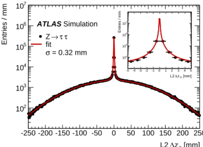
As there is no vertex information available at this stage, an alternative approach is used to reject tracks coming from pile-up interactions. A requirement is
placed on the ∆z0 between a candidate track and the
highest-pT track inside the RoI. The distribution of
∆z0 is shown in Fig. 6 for simulated Z → ττ events
with an average of eight interactions per bunch
cross-ing. High values of ∆z0 typically correspond to pile-up
tracks while the central peak corresponds to the main interaction tracks.
The ∆z0 distribution is fit to the sum of a Breit–
Wigner function to describe the central peak and a Gaussian function to describe the broad distribution from tracks in pile-up events. The half-width of the Breit–Wigner σ=0.32 mm is taken as the point where 68% of the signal events are included in the central peak. A dependence of the trigger variables on
pile-Identification and energy calibration of hadronically decaying tau leptons in ATLAS at 9
up conditions is minimized by considering only tracks
within −2 mm < ∆z0 < 2 mm and ∆R < 0.1 with
respect to the highest-pTtrack.
Track isolation requirements are applied to τhad-vis
candidates to increase background rejection. For multi-track candidates (candidates with two or three associ-ated tracks, defined to be as inclusive as possible with respect to their offline counterpart), the ratio of the
sum of the track pT in 0.1 < ∆R < 0.3 to the sum of
the track pT in ∆R < 0.1 is required to be lower than
0.1. Any 1-track candidate with a reconstructed track in the isolation region is rejected.
In the last step, identification variables combining calorimeter and track information are built as described in Sect. 3.2. The calorimeter-based isolation variable
fcent uses an expanded cone size of ∆R < 0.4
with-out the pile-up correction term to estimate the fraction of transverse energy deposited in the region ∆R < 0.1
around the τhad-viscandidate. The variables ftrackand
Rtrack, measuring respectively the ratio of the
trans-verse momentum of the leading pT track to the total
transverse energy (calibrated at the EM energy scale)
and the pT-weighted distance of the associated tracks
to the τhad-vis direction, are calculated using selected
tracks in the region ∆R < 0.3 around the highest-pT
track. Cuts on the chosen identification variables are optimized to provide an inverse background efficiency of roughly ten while keeping the signal efficiency as high as possible (approximately 90% with respect to the of-fline medium tau identification).
[mm] 0 z ∆ L2 -250 -200 -150 -100 -50 0 50 100 150 200 250 Entries / mm 2 10 3 10 4 10 5 10 6 10 7 10 ATLAS Simulation τ τ → Z fit = 0.32 mm σ [mm] 0 z ∆ L2 -5 -4-3 -2-1 0 1 2 3 4 5 Entries / mm 4 10 5 10 6 10 7 10
Fig. 6 Distribution of ∆z0for the tau trigger at L2 in
sim-ulated Z → ττ events with an average of eight interactions per bunch crossing. The wide Gaussian distribution corre-sponds to pile-up tracks while the central peak, displayed in the upper-right corner, corresponds to the main interaction tracks. A Breit–Wigner function is fitted to the central peak and 68% of the signal events are found within a distance σ = 0.32 mm from the peak.
Event Filter At the EF level, the τhad-vis
reconstruc-tion is very similar to the offline version. First, the TopoCluster reconstruction and calibration algorithms are run within the RoI. Then, track reconstruction in-side the RoI is performed using the EF tracking
algo-rithm. In the last step, the full offline τhad-vis
recon-struction algorithm is used. The EF tracking is almost
100% efficient over the entire pT range with respect
to the offline reconstructed tracks. It is, however, con-siderably slower than the L2 fast tracking algorithm, requiring about 200 ms per RoI under severe pile-up conditions (forty pile-up interactions). The TopoClus-tering algorithms need only about 15 ms.
The τhad-vis candidate four-momentum and input
variables to the EF tau identification are then calcu-lated. The main difference with respect to the offline
tau reconstruction is that π0-reconstruction-based
in-put variables (mπ0+track, Nπ0and pπ
0+track
T /pT) are not
used; the methodology to compute these variables had not yet been developed when the trigger was imple-mented. Furthermore, no pile-up correction is applied to the input variables at trigger level.
Since full-event vertex reconstruction is not avail-able at trigger level (vertices are only formed using the tracks in a given RoI), the selection requirements ap-plied to the input tracks are also different with respect to the offline τhad-visreconstruction. Similarly to L2, the
∆z0requirement for tracks is computed with respect to
the leading track, and loosened to 1.5 mm with respect
to the offline requirement. The ∆d0requirement is
cal-culated with respect to the vertex found inside of the RoI, and is loosened to 2 mm.
A BDT with the input variables listed in Table 2 is used to suppress the backgrounds from jets
misidenti-fied as τhad-vis. The BDT was trained on 1- and 3-track
τhad-vis candidates with simulated Z, W and Z′ events
for the signal and data multi-jet samples for the back-ground, respectively. Only events passing an L1 tau
trigger matched with an offline reconstructed τhad-vis
with pT > 15 GeV and |η| < 2.2 are used, where the
mediumidentification is required for the τhad-vis
candi-dates. For the signal, in addition, a geometrical
match-ing to a true τhad-vis is required. The performance of
the EF tau trigger is presented in Fig. 7. The signal ef-ficiency is defined with respect to offline reconstructed
τhad-vis candidates matched at generator level, and the
inverse background efficiency is calculated in a multi-jet sample. The working points are chosen to obtain a signal efficiency of 85% and 80% with respect to the offline medium candidates for 1-track and multi-track candidates respectively, where the inverse background efficiency is of the order of 200 for the multi-jet sample.
Signal efficiency 0.2 0.3 0.4 0.5 0.6 0.7 0.8 0.9 In ve rs e b a ck g ro u n d e ff ic ie n c y 2 10 3 10 4 10 1-track candidate 2,3-track candidate
ATLAS Data 2012, s=8TeV Tau trigger identification
ta rg e t e ff .
Fig. 7 Inverse background efficiency versus signal efficiency for the tau trigger at the EF level, for τhad-vis candidates
which have satisfied the L1 requirements. The signal effi-ciency is defined with respect to offline medium tau identi-fication τhad-vis candidates matched at generator level, and
the inverse background efficiency is calculated in a multi-jet sample.
3.4 Discrimination against electrons and muons Additional dedicated algorithms are used to
discrim-inate τhad-vis from electrons and muons. These
algo-rithms are only used offline.
Electron veto The characteristic signature of 1-track
τhad-vis can be mimicked by electrons. This creates
a significant background contribution after all the jet-related backgrounds are suppressed via kinematic,
topological and τhad-vis identification criteria. Despite
the similarities of the τhad-vis and electron signatures,
there are several properties that can be used to discrim-inate between them: transition radiation, which is more likely to be emitted by an electron and causes a higher
ratio fHT of high-threshold to low-threshold track hits
in the TRT for an electron than for a pion; the
angu-lar distance of the track from the τhad-vis
calorimeter-based direction; the ratio fEM of energy deposited in
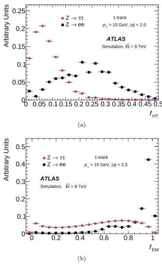
the EM calorimeter to energy deposited in the EM and HAD calorimeters; the amount of energy leaking into the hadronic calorimeter (longitudinal shower informa-tion) and the ratio of energy deposited in the region 0.1 < ∆R < 0.2 to the total core region ∆R < 0.2 (transverse shower information). The distributions for two of the most powerful discriminating variables are shown in Fig. 8. These properties are used to define a
τhad-visidentification algorithm specialized in the
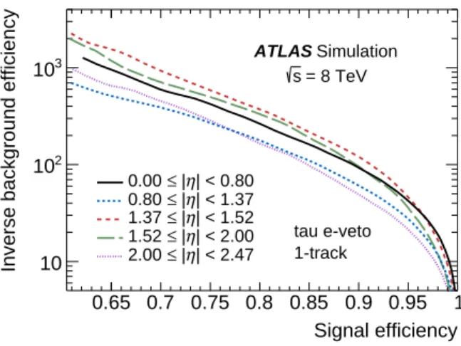
rejec-tion of electrons misidentified as hadronically decaying tau leptons, using a BDT. The performance of this elec-tron veto algorithm is shown in Fig. 9. Slightly different sets of variables are used in different η regions. One of
the reasons for this is that the variable associated with transition radiation (the leading track’s ratio of high-threshold TRT hits to low-high-threshold TRT hits) is not available for |η| > 2.0. Three working points, labelled
tight, mediumand loose are chosen to yield signal
effi-ciencies of 75%, 85%, and 95%, respectively.
HT f 0 0.05 0.1 0.15 0.2 0.25 0.3 0.35 0.4 0.45 0.5 Arbitrary Units 0 0.05 0.1 0.15 0.2 0.25 τ τ → Z ee → Z ATLAS = 8 TeV s Simulation, 1-track | < 2.0 η > 15 GeV, | T p (a) EM f 0 0.2 0.4 0.6 0.8 1 Arbitrary Units 0 0.1 0.2 0.3 0.4 0.5 τ τ → Z ee → Z ATLAS = 8 TeV s Simulation, 1-track | < 2.5 η > 15 GeV, | T p (b)
Fig. 8 Signal and background distribution for two of the electron veto variables, (a) fHT and (b) fEM. Candidate
1-track τhad-vis decays are required to not overlap with a
re-constructed electron candidate which passes tight electron identification [23]. For signal distributions, 1-track τhad-vis
decays are matched to true generator-level τhad-vis in
simu-lated Z → ττ events, while the electron contribution is ob-tained from simulated Z → ee events where 1-track τhad-vis
decays are matched to true generator-level electrons.
Muon veto Tau candidates corresponding to muons can
in general be discarded based on the standard muon identification algorithms [24]. The remaining contam-ination level can typically be reduced to a negligible level by a cut-based selection using the following
char-Identification and energy calibration of hadronically decaying tau leptons in ATLAS at 11
Signal efficiency 0.65 0.7 0.75 0.8 0.85 0.9 0.95 1
Inverse background efficiency 10
2 10 3 10 | < 0.80 η | ≤ 0.00 | < 1.37 η | ≤ 0.80 | < 1.52 η | ≤ 1.37 | < 2.00 η | ≤ 1.52 | < 2.47 η | ≤ 2.00 ATLAS Simulation = 8 TeV s tau e-veto 1-track
Fig. 9 Electron veto inverse background efficiency versus signal efficiency in simulated samples, for 1-track τhad-vis
candidates. The background efficiency is determined using simulated Z → ee events.
acteristics. Muons are unlikely to deposit enough
en-ergy in the calorimeters to be reconstructed as τhad-vis
candidates. However, when a sufficiently energetic clus-ter in the calorimeclus-ter is associated with a muon, the muon track and the calorimeter cluster together may be
misidentified as a τhad-vis. Muons which deposit a large
amount of energy in the calorimeter and therefore fail muon spectrometer reconstruction are characterized by a low electromagnetic energy fraction and a large ratio
of track-pT to ET deposited in the calorimeter.
Low-momentum muons which stop in the calorimeter and overlap with calorimeter deposits of different origin are characterized by a large electromagnetic energy fraction
and a low pT-to-ETratio. A simple cut-based selection
based on these two variables reduces the muon contam-ination to a negligible level. The resulting efficiency is
better than 96% for true τhad-vis, with a reduction of
muons misidentified as τhad-visof about 40%. However,
the performance can vary depending on the τhad-visand
muon identification levels.
4 Efficiency measurements using Z tag-and-probe data
To perform physics analyses it is important to measure the efficiency of the reconstruction and identification algorithms used online and offline with collision data.
For the τhad-vissignal, this is done on a sample enriched
in Z → ττ events. For electrons misidentified as a tau signal (after applying the electron veto) this is done on a sample enriched in Z → ee events.
The chosen tag-and-probe approach consists of se-lecting events triggered by the presence of a lepton
(tag) and containing a hadronically decaying tau lepton candidate (probe) in the final state and extracting the efficiencies directly from the number of reconstructed
τhad-vis before and after tau identification algorithms
are applied. In practice, it is impossible to obtain a pure sample of hadronically decaying tau leptons, or electrons misidentified as a tau signal, and therefore backgrounds have to be taken into account. This is de-scribed in the following sections.
4.1 Offline tau identification efficiency measurement To estimate the number of background events for the purpose of tau identification efficiency measurements, a variable with high separation power, which is
mod-elled well for simulated τhad-vis decays is chosen: the
sum of the number of core and outer tracks associated to the τhad-viscandidate. Outer tracks in 0.2 < ∆R < 0.6 are only considered if they fulfill the requirement
Douter = min([ pcore
T /pouterT ] · ∆R(core, outer)) < 4,
where pcore
T refers to any track in the core region, and
∆R(core, outer) refers to the distance between the can-didate outer track and any track in the core region. This requirement suppresses the contribution of outer tracks from underlying and pile-up events, due to re-quirements on the relative momentum and separation of the tracks. This allows the signal track multiplicity to retain the same structure as the core track multiplic-ity distribution. For backgrounds from multi-jet events, the track multiplicity is increased by the addition of tracks with significant momentum in the outer cone.
The requirement on Douter was chosen to offer
opti-mal signal to background separation. A fit is then per-formed using the expected distributions of this variable
for both signal and background to extract the τhad-vis
signal. This fit is performed for each exclusive tau iden-tification working point, corresponding to: candidates failing the loose requirement, candidates satisfying the
looserequirement but failing the medium requirement,
candidates satisfying the medium requirement but fail-ing the tight requirement and candidates satisfyfail-ing the
tightrequirement.
4.1.1 Event selection
Z → τlepτhad events are selected by a triggered muon
or electron coming from the leptonic decay of a tau lep-ton, and the hadronically decaying tau lepton is then searched for in the rest of the event, considered as the
probe for the tau identification performance
measure-ment. These events are triggered by a single-muon or a single-electron trigger requiring one isolated trigger
Offline, muons and electrons with pT> 26 GeV are thereafter selected, representing the tag objects. Addi-tional track and calorimeter isolation requirements are applied to the muon and electron. Identified muons are required to have |η| < 2.4. Identified electrons are re-quired to have |η| < 1.37 or 1.52 < |η| < 2.47, therefore excluding the poorly instrumented region at the inter-face between the barrel and endcap calorimeters. In ad-dition to the requirement of exactly one isolated muon
or electron (ℓ), a τhad-vis candidate is selected in the
kinematic range pT > 15 GeV and |η| < 2.5, requiring
one or three associated tracks in the core region and an absolute electric charge of one and no geometrical
overlap with muons with pT> 4 GeV or with electrons
with pT> 15 GeV of loose or medium quality
(depend-ing on η). For τhad-viswith one associated track, a muon
veto and a medium electron veto is applied. In addition to this, a very loose requirement on the tau identifica-tion BDT score is made which strongly suppresses jets while being more than 99% efficient for Z → ττ sig-nal. The tag and the probe objects are required to have opposite-sign electric charges (OS).
Additional requirements are made in order to
sup-press (Z → ℓℓ) + jets and (W → ℓνℓ) + jets events:
– On the invariant mass calculated from the lepton and the τhad-visfour-momenta (mvis(ℓ, τhad-vis)): for pτhad-vis
T < 20 GeV, 45 GeV < mvis(ℓ, τhad-vis) <
80 GeV. Otherwise, for the µ channel, 50 GeV < mvis(µ, τhad-vis) < 85 GeV, and for the e channel: 50 GeV < mvis(e, τhad-vis) < 80 GeV. For the sig-nal, this variable peaks in these regions.
– On the transverse mass of the lepton and Emiss
T
system (mT=
q 2pℓ
T· ETmiss(1 − cos ∆φ(ℓ, ETmiss))):
mT < 50 GeV. For most backgrounds (e.g.
(W → ℓνℓ) + jets), this variable peaks at larger
values.
– On the distance in the azimuthal plane between
the lepton and Emiss
T (neutrinos) and between the
τhad-vis and ETmiss (Σ cos ∆φ = cos ∆φ(ℓ, ETmiss) +
cos ∆φ(τhad-vis, ETmiss)): Σ cos ∆φ > −0.15. For the signal, this variable tends to peak at zero, indicating that the neutrinos point mainly in the direction of one of the two leptons from Z decay products. For W + jets background events, the value is typically negative, indicating that the neutrino points away from the two lepton candidates.
4.1.2 Background estimates and templates
The signal track multiplicity distribution is modelled
using simulated Z → τlepτhad events. Only
recon-structed τhad-vis matched to a true hadronic tau decay
are considered.
A single template is used to model the background from quark- and gluon-initiated jets that are misidenti-fied as hadronic tau decays. The background is mainly composed of multi-jet and W +jets events with a mi-nor contribution from Z+jets events. The template is constructed starting from a enriched multi-jet control region in data that uses the full signal region selection but requires that the tag and probe objects have same-sign charges (SS). The contributions from W +jets and Z+jets in the SS control region are subtracted. The template is then scaled by the ratio of OS/SS multi-jet events, measured in a control region which inverts the very loose identification requirement of the signal region. Finally, the OS contributions from W +jets and Z+jets are added to complete the template. The Z+jets contribution is estimated using simulated samples. The shape of the W +jets contribution is estimated from a high-purity W +jets control region, defined by
remov-ing the mTrequirement and inverting the requirement
on Σ cos ∆φ. The normalization of the W +jets contri-bution is estimated using simulation.
An additional background shape is used to take into account the contamination due to misidentified elec-trons or muons. This small background contribution (stemming mainly from Z → ℓℓ events) is modelled by taking the shape predicted by simulation using
can-didates which are not matched to true τhad-visin events
of type Z → τlepτhad, t¯t, diboson, Z → ee, µµ where
the reconstructed tau candidate probe is matched to a electron or muon. For the fit, the contribution of these backgrounds is fixed to the value predicted by the simu-lation, which is typically less than 5% of the total signal yield.
To measure both the 1-track and 3-tracks τhad-vis
efficiencies, a fit of the data to the model (signal plus background) is performed, using two separate signal templates. The signal templates are obtained by requir-ing exactly one or three tracks reconstructed in the core
region of the τhad-viscandidate. To improve the fit
sta-bility in the background-dominated region where the tau candidates fail the loose requirements, the ratio of the 1-track to 3-track normalization is fixed to the value predicted by the simulation. For other exclusive regions, the ratio is allowed to vary during the fit.
In the fit to extract the efficiencies for real tau lep-tons passing different levels of identification, the ratio
of jet to other τhad-vis candidates is determined in a
preselection step (where no identification is required) and then extrapolated to regions where identification is required by using jet misidentification rates determined in an independent data sample.
Identification and energy calibration of hadronically decaying tau leptons in ATLAS at 13
4.1.3 Results
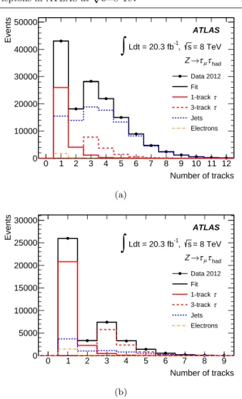
Figure 10 shows an example of the track multiplicity distribution after the tag-and-probe selection, before and after applying the tau identification requirements, with the results of the fit performed. The peaks in the one- and three-track bins are due to the signal contri-bution. These are visible before any identification re-quirements are applied, and become considerably more prominent after identification requirements are applied, due to the large amount of background rejection pro-vided by the identification algorithm. To account for the small differences between data and simulations, correc-tion factors, defined as the ratio of the efficiency in data to the efficiency in simulation for τhad-vissignal to pass a certain level of identification, are derived. Their val-ues are compatible with one, except for the tight 1-track working point, where the correction factor is about 0.9.
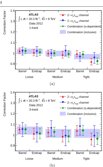
Results from the electron- and muon-tag analysis are combined to improve the precision of the correction factors, shown in Fig. 11. No significant dependency on
the pTof the τhad-visis observed and hence the results
are provided separately only for the barrel (|η| < 1.5) and the endcap (1.5 < |η| < 2.5) region, and for one and three associated tracks. Uncertainties depend slightly on the tau identification level and kinematic quanti-ties. In Table 3, the most important systematic uncer-tainties for the working point used by most analyses,
mediumtau identification, are shown, together with the
total statistical and systematic uncertainty. Uncertain-ties due to the underlying event (UE) are the domi-nant ones for the signal template, and are estimated by comparing alpgen-Herwig and Pythia simulations. The shower model and the amount of detector material are also varied and included in the number reported in Table 3. The W +jets shape uncertainty accounts for differences between the W +jets shape in the signal and control regions and is derived from comparisons to simulated W +jets events. The jet background fraction uncertainty accounts for the effect of propagating the statistical uncertainty on the jet misidentification rates.
The results apply to τhad-vis candidates with pT >
20 GeV. For pT < 20 GeV, uncertainties increase to
a maximum of 15% for inclusive τhad-vis candidates.
For pT > 100 GeV, there are no abundant sources of
hadronic tau decays to allow for an efficiency
measure-ment. Previous studies using high-pT dijet events
in-dicate that there is no degradation in the modelling of tau identification in this pTrange, within the statistical uncertainty of the measurement [14].
Number of tracks 0 1 2 3 4 5 6 7 8 9 10 11 12 Events 0 10000 20000 30000 40000 50000 Data 2012 Fit τ 1-track τ 3-track Jets Electrons ATLAS -1 Ldt = 20.3 fb ,
∫
s = 8 TeV had τ µ τ → Z (a) Number of tracks 0 1 2 3 4 5 6 7 8 9 Events 0 5000 10000 15000 20000 25000 30000 Data 2012 Fit τ 1-track τ 3-track Jets Electrons ATLAS -1 Ldt = 20.3 fb ,∫
s = 8 TeV had τ µ τ → Z (b)Fig. 10 Template fit result in the muon channel, inclusive in η and pT for pT> 20 GeV for the offline τhad-vis
candi-dates (a) before the requirement of tau identification, and (b) fulfilling the medium tau identification requirement.
Source Uncertainty [%]
1-track 3-track
Jet background fraction 0.8 1.5
Jet template shape 0.9 1.4
Tau energy scale 0.7 0.8
Shower model/UE 1.8 2.5
Statistics 1.0 2.2
Total 2.5 4.0
Table 3 Dominant uncertainties on the medium tau identi-fication efficiency correction factors estimated with the Z tag-and-probe method, and the total uncertainty, which combines systematic and statistical uncertainties. These uncertainties apply to τhad-vis candidates with pT> 20 GeV.
Barrel Endcap Barrel Endcap Barrel Endcap Correction Factor 0.9 1 1.1 1.2 1.3 1.4
Loose Medium Tight
ATLAS = 8 TeV s , -1 L dt = 20.3 fb ∫ Data 2012 1-track channel had τ µ τ → Z channel had τ e τ → Z -dependent) η Combination ( Combination (inclusive) (a)
Barrel Endcap Barrel Endcap Barrel Endcap
Correction Factor 0.9 1 1.1 1.2 1.3 1.4
Loose Medium Tight
ATLAS = 8 TeV s , -1 L dt = 20.3 fb ∫ Data 2012 3-track channel had τ µ τ → Z channel had τ e τ → Z -dependent) η Combination ( Combination (inclusive) (b)
Fig. 11 Correction factors needed to bring the offline tau identification efficiency in simulation to the level observed in data, for all tau identification working points as a function of η. The combinations of the muon and electron channels are also shown, and the results are displayed separately for (a) 1-track and (b) 3-track τhad-vis candidates with pT> 20
GeV. The combined systematic and statistical uncertainties are shown.
4.2 Trigger efficiency measurement
The tau trigger efficiency is measured with Z → ττ events using tag-and-probe selection similar to the one described in Sect. 4.1. The only difference is that the efficiency is measured with respect to identified offline
τhad-vis candidates and thus, offline tau identification
selection criteria are applied during the event selection. Only the muon channel is considered, as the background contamination is smaller than in the electron channel. The statistical uncertainty improvements that could be obtained by the addition of the electron channel are offset by the larger systematic uncertainties associated with this channel. The systematic uncertainties are also different from those in the offline identification mea-surement, since the purity after identification is already
high. The systematics are dominated by the uncertain-ties on the modelling of the kinematics of the back-ground events, rather than the total normalization, as is the case for the offline identification measurement.
The dominant background contribution is due to W + jets and multi-jet events, where a jet is misidentified
as a τhad-vis. These backgrounds are estimated using a
method similar to the one described in Sect. 4.1.2. The same multi-jet and W + jets control regions are used. The shape of other backgrounds is taken from simu-lation but the normalizations of the dominant back-grounds are estimated from data control regions. The contribution of top quark events is normalized in a con-trol region requiring one jet originating from a b-quark. Z+jets events with leptonic Z decays and one of the
additional jets being misidentified as τhad-vis are
nor-malized by measuring this misidentification rate in a control region with two identified oppositely charged same-flavour leptons.
In total, more than 60,000 events are collected, with a purity of about 80% when the offline medium tau identification requirement is applied. With the addition of the tau trigger requirement, the purity increases to about 88%. Most of the backgrounds accumulate in the region pT< 30 GeV.
Figure 12 shows the measured tau trigger efficiency
for τhad-vis candidates identified by the offline medium
tau identification as functions of the offline τhad-vis
transverse energy and the number of primary vertices in the event, for each level of the trigger. The tau trigger
considered has calorimetric isolation and a pTthreshold
of 11 GeV at L1, a 20 GeV requirement on pT, the
num-ber of tracks restricted to three or less, and medium se-lection on the BDT score at EF. The efficiency depends
minimally on pT for pT > 35 GeV or on the pile-up
conditions. The measured tau trigger efficiency is com-pared to simulation in Fig. 13; the efficiency is shown to be modelled well in simulation. Correction factors, as defined in Sect. 4.1, are derived from this measure-ment. The correction factors are in general compatible
with unity, except for the region pT< 40 GeV where a
difference of a few per cent is observed.
In the pT range from 30 GeV to 50 GeV, the
un-certainty on the correction factors is about 2% but
in-creases to about 8% for pT= 100 GeV. The uncertainty
is also sizeable in the region pT < 30 GeV, where the
background contamination is the largest. 4.3 Electron veto efficiency measurement
To measure the efficiency for electrons reconstructed as
τhad-vis to pass the electron veto in data, a
Identification and energy calibration of hadronically decaying tau leptons in ATLAS at 15 [GeV] T p Offline tau 0 20 40 60 80 100 E ffi c ie nc y 0 0.2 0.4 0.6 0.8 1 L1 L1 + L2 L1 + L2 + EF -1 Ldt = 20.3 fb ,
∫
s = 8 TeV ATLAS had τ µ τ → Data 2012, Z 20 GeV tau trigger(a)
Number of primary vertices
0 5 10 15 20 25 E ffi c ie n c y 0 0.2 0.4 0.6 0.8 1 L1 L1 + L2 L1 + L2 + EF -1 Ldt = 20.3 fb ,
∫
s = 8 TeV ATLAS had τ µ τ → Data 2012, Z 20 GeV tau trigger(b)
Fig. 12 The tau trigger efficiency for τhad-vis candidates
identified by the offline medium tau identification, as a func-tion of (a) the offline τhad-vis transverse energy and (b) the
number of primary vertices. The error bars correspond to the statistical uncertainty in the efficiency.
events, as illustrated in Fig. 14 (a). The measurement
uses probe 1-track τhad-vis candidates in the opposite
hemisphere to the identified tag electron. The tag elec-tron is required to fulfil ptagT > 35 GeV in order to sup-press backgrounds from Z → ττ events. The probe is required not to overlap geometrically with an identified electron, e.g. in the case of Fig. 14 a loose electron iden-tification is used. Different veto algorithms are tested in combination with different levels of jet discrimination, and the effects estimated. Efficiencies are extracted
di-rectly from the number of reconstructed τhad-visbefore
and after identification, in bins of η of the τhad-vis can-didate, after subtracting the background modelled by simulation (normalized to data in dedicated control re-gions). The shape and normalization of the multi-jet
background distribution for the η of the τhad-visare
es-timated using events with SS tag electron and probe
τhad-vis in data after subtracting backgrounds in the
SS region using simulation. To estimate the W → eν, Z → ττ, and t¯t backgrounds, the shape of this
distri-E ff ic ie n c y 0 0.1 0.2 0.3 0.4 0.5 0.6 0.7 0.8 0.9 1 Data 2012 Sim. Z→ττ Data stat. error Sim. stat. error Data sys. error
-1 Ldt = 20.3 fb
∫
= 8 TeV s ATLAS20 GeV tau trigger had τ µ τ → Z [GeV] T p Offline tau 0 20 40 60 80 100 Sim. ε / Data ε 0.8 0.9 1 1.1 1.2 Stat. (Data) Stat. (Sim.) Sys.
Fig. 13 The measured tau trigger efficiency in data and sim-ulation, for the offline τhad-viscandidates passing the medium
tau identification, as a function of offline τhad-vis transverse
energy. The expected background contribution has been sub-tracted from the data. The uncertainty band on the ratio reflects the statistical uncertainties associated with data and simulation and the systematic uncertainty associated with the background subtraction in data.
bution is obtained from simulation but normalized to dedicated data control regions for each background.
Differences in the modelling of the electron veto al-gorithm’s performance in simulation compared to data are parameterized as correction factors in bins of η of
the τhad-vis candidate, by comparing distributions
sim-ilar to the one shown in Fig. 14 (b).
Uncertainties on the correction factors (which are typically close to unity) are η-dependent and amount to about 10% for the loose electron veto and get larger for the medium and tight electron veto working points, mainly driven by statistical uncertainties. A summary of the main uncertainties for the working point shown in Fig. 14 is provided in Table 4.
Source Uncertainty [%]
Tag selection (pT, isolation) 5–28
Background rejection 1–8
Statistics 7–12
Total 8–30
Table 4 Dominant uncertainties on the loose electron veto efficiency correction factors estimated with the Z tag-and-probe method. The range of the uncertainties reflects their variation with η.