Undertaking specific parameters : implementation of the EIOPA Guidelines

M

ASTER OF

S

CIENCE IN

A

CTUARIAL

S

CIENCES

M

ASTERS

F

INAL

W

ORK

I

NTERNSHIP

R

EPORT

U

NDERTAKING

S

PECIFIC

P

ARAMETERS

:

IMPLEMENTATION OF THE

EIOPA

G

UIDELINES

A

NA

S

AMUEL

B

ARROQUEIRO

M

ARQUES

R

ODRIGUES

M

ASTER OF

S

CIENCE IN

A

CTUARIAL

S

CIENCES

M

ASTERS

F

INAL

W

ORK

I

NTERNSHIP

R

EPORT

U

NDERTAKING

S

PECIFIC

P

ARAMETERS

:

IMPLEMENTATION OF THE

EIOPA

G

UIDELINES

A

NA

S

AMUEL

B

ARROQUEIRO

M

ARQUES

R

ODRIGUES

S

:

J

A

S

P

I

i

Preface

This work is the result of a five-month curricular internship taken at KPMG Advisory – Consultores de Gestâo S.A., for the completion of the Master in Actuarial Sciences. During the internship, I had the job of evaluate the draft methodologies defined for the Undertaking Specific Parameters (USP) and it´s applicability in a real world context. The USP for premium and reserve risk were estimated according to the draft Guidelines of EIOPA.

I wish to thank KPMG for making my internship possible, and all the people there that help me in these few months, especially to Pedro Inês for his guidance and help throughout the entire project. A special thanks for my supervisor in ISEG, João Andrade e Silva, for helping me whenever I needed.

Finally, I would also to show my gratitude to my parents and brother for all the support and encouragement, and also to my friends who I can always count on.

ii

Abstract

Under the new Solvency II regime, in order to be able to cover their risks and therefore protect their policyholders, insurers and reinsurers are required to calculate their Solvency Capital Requirement. To do this, insurers can opt to use the Standard Formula, an internal model or to substitute some of the Standard Formula parameters with Undertaking Specific Parameters.

This work aims at estimating the Undertaking Specific Parameters of the non-life premium and reserve risk sub-module, for a specific Line of Business of a Portuguese insurer. In order to do so, the standardized methods provided by the European Insurance and Occupational Pensions Authority were applied. The results obtained were compared with the parameters provided by the Standard Formula for this line of business.

Keywords

Solvency II, Undertaking Specific Parameters, Reserve Risk, Premium Risk, Standard Formula, Solvency Capital Requirement, Chain Ladder, Merz-Wüthrich, Double Chain Ladder.

iii

Acronyms

BSCR: Basic Solvency Capital Requirement CDR: Claims Development Result

CL: Chain Ladder

DCL: Double Chain Ladder

EIOPA: European Insurance and Occupational Pensions Authority EU: European Union

FLAOR: Forward Looking Assessment of Own Risks IBNR: Incurred But Not Reported

ISP: Instituto de Seguros de Portugal LoB: Line of Business

LTGA: Long Term Guarantees Assessment MCR: Minimum Capital Requirement

MSEP: Mean Square Error of Prediction NSLT: Non-Similar to Life Techniques

ORSA: Own Risk and Solvency Assessment QIS: Quantitative Impact Study

RBNS: Reported But Not Settle SCR: Standard Capital Requirement SLT: Similar to Life Techniques

iv

Index

3. Solvency Capital Requirement ... 6

3.1. Standard Formula ... 8

3.1.1. Standard Formula with Simplifications ... 9

3.1.2. Standard Formula with Undertaking Specific Parameters ... 9

3.2. Internal Models... 11

4. Non-life Underwriting Risk ... 12

4.1. The Standard Formula ... 12

4.1.1. Premium and Reserve Risk sub module and Standard Parameters ... 13

4.1.2. Standard Parameters for Fire and Other Damages to Property ... 15

4.2. Undertaking Specific Parameters ... 15

4.2.1. Delegated Acts ... 15

4.2.1.1.Premium Risk ... 15

4.2.1.2. Reserve Risk ... 17

4.2.2. Consultation Papers ... 18

4.2.2.1.Premium Risk ... 18

4.2.2.1.1. Method 1 – Historical Loss Ratio ... 19

4.2.2.1.2. Method 2 – Lognormal Distribution Loss Ratio ... 20

4.2.2.1.3. Method 3 – Swiss Solvency Ratio ... 21

4.2.2.1.4. Comparison between Methods ... 22

4.2.2.2. Reserve Risk ... 23

4.2.2.2.1. Method 1 – Retrospective Method ... 23

4.2.2.2.2. Method 2 – MSEP and DCL ... 25

4.2.2.2.3. Method 3 – MSEP and CL ... 25

4.2.2.2.4. Comparison between Methods ... 26

v

5.1. Mack Model ... 27

5.2. Merz-Wüthrich ... 28

5.3. Double Chain Ladder ... 29

6. Application to the Real World Context ... 31

6.1. Delegated Acts ... 31 6.1.1. Premium Risk ... 31 6.1.2. Reserve Risk ... 32 6.2. Consultation Papers ... 32 6.2.1. Premium Risk ... 32 6.2.2. Reserve Risk ... 33 6.3. Results ... 34

7. Conclusions and Further Developments ... 35

Annexes ... 36

Annex 1. Representation of the Standard Formula ... 36

Annex 2. Correlation Matrixes ... 37

Annex 3. Credibility Factor ... 39

Annex 4. Standard Parameters for Premium and Reserve Risk ... 40

Annex 5. Calculation of the Var(Θ) ... 41

Annex 6. Example on how to obtain the Input for Premium Risk ... 42

Annex 7. Example on how to obtain the Input for Reserve Risk ... 43

Annex 8. Using the R Package “Double Chain Ladder” ... 44

vi

List of Figures

Figure 1. Solvency II Regime Timeline ... 6 Figure 2. Relation between SF, Simplifications and USP ... 10

List of Tables

Table 1. Comparison of the USP for Premium Risk for the different methods ... 3334 Table 2. Comparison of the USP for Reserve Risk for the different methods ... 34

1

1. Introduction

The insurance business is a risk management business. Due to its importance the insurance market must be under an adequate supervisory regime. In the 70’s the European Union launched the first Directives, and since then the legislative process has changed along the years until the Solvency II regime that is being prepared.

Solvency II is a new regulatory regime for the European insurance and reinsurance market. It aims to establish more harmonized requirements across the EU, thus fomenting competitive equality as well as more and higher uniform levels of consumer protection. Under the Solvency II regime insurers must hold sufficient available resources to secure the Solvency Capital Requirement (SCR). The SCR covers the main categories of risks that an insurer faces, and it is set at a level to ensure that the undertaking is able to meet its obligations, over the next 12 months, with a probability of 99.5%, meaning that the chance of being insolvent is no more than 1 in 200. The SCR may be derived using either the Standard Formula or an approved internal model.

The internal model allows the insurer to model its risks and therefore to measure its capital requirements taking into account its own specificities. However, this approach requires much resources, and is subject to approval of the supervisory authorities. The Standard Formula (SF), on the other hand, is a more simple methodology and process that was developed to reflect and European Insurance Company with an average risk and will be used for most of the market.

Companies with a risk profile which is not well represented by the SF, and do not want to implement an internal model, can use a more developed approach of the SF: the Undertaking Specific Parameters (USP). USP do not take excessive calculation time, and

2

yet, allows a better assessment of the undertaking risk when compared to the SF. However, only some sub-modules of the Standard Formula can have their parameters replaced by USP.

One of the risks where the USP can substitute the SF parameters is the non-life premium and reserve risk. Article 105 of the Solvency II Directive 2009/138/EC, defines this risk sub-module as: «the risk of loss, or of adverse change in the value of insurance liabilities,

resulting from fluctuations in the timing, frequency and severity of insured events, and in

the timing and amount of claim settlements».

This work will start with a brief framework on Solvency II regime and the Standard Formula. Afterwards, we will present a detailed explanation of the methods, provided by EIOPA in the draft Delegated Acts and in the Consultation Papers, to calculate the USP for both premium and reserve risks. Finally we will present the results of an application of those methods to a real world context.

2. Solvency II

The insurance business is by definition a risk management business. The inverted production cycle and the existence of some branches of the business with long periods of coverage and liabilities, makes extremely important that the insurance and reinsurance market is under an adequate supervisory regime. In this context, the objective of a solvency regime is to ensure the financial soundness of insurance undertakings and their capability to survive difficult times, thus protecting the policyholders and the stability of the market.

The EU insurance legislative framework started in the 70’s, with a set of Directives known as the 1st _{Council Directives. These Directives defined the Provisions that the life and}

3

non-life branches must hold and also the abolition of the restrictions on freedom of establishment in the Member States. This primary framework ended in the beginning of the 90’s with the 3rd _{Council Directives that emend the previous ones and determined that} insurance companies only needed a unique authorization by the Member State of origin to be able to establish in any other Member State. After a revision of the solvency rules, the Commission proceeded to a quick but limited modification, which gave origin to new Directives launched in 2002, called Solvency I.

However, Solvency I was always seen as a transitional regime, therefore certain areas required improvement, such as the lack of harmonization in the valuation of assets and in the calculation of technical provisions, the fact that there was no recognition of the positive effect of risk diversification and very little recognition of reinsurance, especially non-proportional treaties. Although the principal limitation of Solvency I is the lack of sensibility of the regime to the risks of insurance undertakings, or even the absence of capital requirements to cover important risks like market, credit and operational risks. The necessity of a new Solvency regime became clear, and in 2009 the Solvency II Directive was published. Solvency II is a new regulatory regime being implemented in order to harmonize the EU insurance and reinsurance market. Solvency II requirements will be more comprehensive and will be a total balance sheet type of regime where all the risks and their interactions will be considered.

2.1. The Pillars

The Solvency II regime is organized into three main areas that group the requirements needed, these areas are called pillars.

4

 Pillar 1 – Quantitative requirements: The first pillar covers all the quantitative requirements, and aims to ensure that firms are adequately capitalized with risk-based capital. It provides harmonized standards for the valuation of assets, technical provisions and other liabilities, classification and eligibility of own funds and two capital thresholds (SCR and MCR). These quantitative requirements are still being discussed, and therefore aren’t fully settled. In order to test the practicability, the implications and impacts of proposed new requirements and technical specifications on insurers and reinsurers financial resources, EIOPA requested various exercises throughout the time. These exercises are called Quantitative Impact Study, and until now six QIS were carried out: QIS 1 (2005), QIS 2 (2006), QIS 3 (2007), QIS 4 (2008), QIS 5 (2010) and LTGA (2013). In June 2014, EIOPA launched a Stress Test to evaluate the resilience of insurers regarding market risk under a combination of historical and hypothetical scenarios, additionally insurance risk will be tested. Instituto de Seguros de Portugal (ISP), the supervisory authority in Portugal, taking advantage of this Stress Test also launched the QIS 2014 at a national level. QIS 2014 is directed to identify the vulnerability areas, not only on the reduction of the risks and the capital needs but also to assess the capacity of the undertakings to perform the calculations in an adequate manner.

 Pillar 2 – Qualitative requirements: Pillar II imposes higher standards of risk management and governance within a firm’s organization. There is two different dimensions of risk management, the first one is the operational risk management that guarantees an adequate management and the integration of principles and mechanisms of risk management in the everyday life of the organizations, through the

5

implementation of a system of governance, politics and key functions. The other one, the strategic risk management, identifies and evaluates the capital taking into account the risks arising from the business and from the company’s strategy. It is the Own Risk and Solvency Assessment (ORSA).

 Pillar 3 – Supervisory reporting and public disclosure: This pillar focuses on disclosure requirements to ensure the transparency both for supervisors and for the public and to enhance market discipline. It is based on two types of report, one is the Regulatory Supervisory Report, which is a private report to be submitted to the supervisory authority, and follows from article 35 of the Directive, and the other is the Solvency and Financial Condition Report, which is public and follows from article 51.

2.2. Legislative Process

Solvency II was developed under the Lamfalussy Process, which is a four level approach. The first level is composed by the Omnibus II Directive that was proposed by the European Commission on January 2011. This new Directive was already approved and it emends the Solvency II Directive according to the Lisbon Treaty. Level 2 is defined as the Implementing Measures – Delegated Acts and is adopted by the Commission and lays down the detailed rules of the Solvency II regime. The level 2.5 is the Technical Standards developed by EIOPA and approved by the Commission and details technical rules, therefore no strategic decisions or political choices should be incorporated in this stage. The third level is composed by Guidelines issued by EIOPA to supervisors and undertakings to ensure consistent implementation and cooperation between Member States. Finally, level 4 incorporates a rigorous enforcement of Community legislation by

6

the Commission. The following timeline presents the calendar for the whole legislative process since the adoption of the Omnibus II Directive.

Figure 1: Solvency II regime timeline

Source: EIOPA

3. Solvency Capital Requirement

The basis for the Solvency II framework is the Total Balance Sheet Approach. This means that the determination of an insurer’s ability to cover its obligations must be based upon its total financial position and that assets and liabilities must be valued at market value. Insurers are able to cover their obligations if their solvency ratio is bigger than 1, this ratio is defined as the ratio between the eligible capital, obtained using the eligible own funds, and the required capital which is defined with the two thresholds – Solvency Capital Requirement and Minimum Capital Requirement.

Own funds defines the capital available to the insurer to create new business and to serve as a buffer to absorb unexpected losses. It includes basic own funds and ancillary own

• Adoption of the Omnibus II Directive December 2013

• Public consultation on the Set 1 of the ITS April– June 2014

• Public consultation on the Set 1 of the Guidelines June– September 2014

• Submition to the European Commission of the Set 1 of the ITS

31 October 2014

• Public consultation on the Set 2 of the ITS • Public consultation on the Set 2 of the Guidelines December 2014 – March

2015

• Publication of the Set 1 of the Guidelines February 2015

• Submission to the European Commission of the Set 2 of the ITS

30 June 2015

• Publication of the Set 2 of the Guidelines July 2015

• Application of the Solvency II regime 1 January 2016

7

funds that are classified into tiers numbered from 1 (higher quality funds) to 3 (lower quality funds) based on subordination and permanent availability. The eligible amount of Tier 1 items shall be at least 50% of the SCR and 80% of the MCR, and the eligible amount of Tier 3 item shall be less than 15% of the SCR.

The SCR is the amount of capital to be held by insurers and reinsurers undertakings in order to avoid insolvency. It should take into account all the quantifiable risks that undertakings are exposed to and it must cover unexpected losses of the existing business as well as the new business expected to be written in the next 12 months. According to Article 101 (3), «it shall correspond to the Value-at-Risk of the basic own funds of an

insurance or reinsurance undertaking subject to a confidence level of 99.5% over a

one-year period».

The Minimum Capital Requirement defines the level of own funds from which the risk of insolvency is considered excessive and it defines also the trigger for severe measures from the supervisory authorities. The calculation of the MCR combine a linear formula with a floor of 25% and a cap of 45% of the SCR and an absolute minimum depending on the nature of the undertaking.

The Solvency II regime allows the undertakings to use the method that better reflect their risk complexity to calculate the Solvency Capital Requirement. In this context, the principle of proportionality is very important, in Article 28 is defined that «Member States

shall ensure that the requirements (…) are applied in a manner which is proportionate to the nature, scale and complexity of the risk inherent in the business of an insurance or

reinsurance undertaking». EIOPA proposes five methods to calculate the SCR that can

8

3.1. Standard Formula

The Standard formula is developed to reflect one European insurance undertaking with an average risk. It is a risk-based mathematical formula that categorizes risks into risk modules for capital purposes, with an allowance for aggregation and diversification across modules. It has a modular structure which combines the following risk modules: operational risk, adjustment and Basic Solvency Capital Requirement (BSCR), where the last one is divided into six sub-modules: market risk, counterparty default risk, life underwriting risk, non-life underwriting risk, health underwriting risk and intangible assets risk. A representation of the SF is presented in Annex 1.

The Formula Standard and its risks are calibrated in such a way that ensures the SCR «correspond to the Value-at-Risk of the basic own funds of an insurance or reinsurance

undertaking subject to a confidence level of 99.5% over a one-year period», (Article 101).

The overall standard formula capital requirement is given by the sum of the adjustment for the risk absorbing effect and the capital requirements for the BSCR and the operational risk. The scope of this work is only on the non-life underwriting risk module that belongs to BSCR, so only the formula for the calculation of the BSCR will be presented:

𝐵𝑆𝐶𝑅 = √∑ 𝐶𝑜𝑟𝑟𝑖𝑗 × 𝑆𝐶𝑅𝑖× 𝑆𝐶𝑅𝑗 𝑖,𝑗

+ 𝑆𝐶𝑅_{𝑖𝑛𝑡𝑎𝑛𝑔𝑖𝑏𝑙𝑒}

Where:

 Corrij represents the entries of the correlation matrix Corr (see Annex 2);

 SCRi and SCRj represent the capital requirements for the individual risks according to

9

3.1.1. Standard Formula with Simplifications

Undertakings can use a «simplified calculation for a specific risk module or sub-module

where the nature, scale and complexity of the risk they face justifies it and where it would

be disproportionate to apply the standardized calculation» (Article 109). However,

simplifications can only be used in some risks, as for instance: life and health mortality risk, life and health longevity risk and life catastrophe risk.

3.1.2. Standard Formula with Undertaking Specific Parameters

When calculating the SCR, if the undertaking risk profile cannot be adequately reflected by the Standard Formula, insurance undertakings may «within the design of the Standard

Formula, replace a subset of its parameters by parameters specific to the undertaking»,

as set out in Article 104 (7).

The subset of USP authorized by EIOPA are:

 Non-life premium and reserve parameters: standard deviation for premium risk and standard deviation for reserve risk;

 NSLT health premium and reserve risk parameters: standard deviation for premium risk and standard deviation for reserve risk;

 SLT health revision risk: replace a standard parameter of revision shock;

 Revision risk on SCR life risk module: replace a standard parameter of revision shock.

For all others parameters, undertakings shall use the values of Standard Formula parameters.

In order to obtain each USP, EIOPA parameterized all the calculations and provides standardized methods that must be used by all the undertakings. The use of Undertaking

10

Specific Parameters is subject to supervisory approval, during this process «supervisory

authorities shall verify the completeness, accuracy and appropriateness of the data

used», (Article 104 (7)) as well as verify the additional data requirements of each

individual method. Supervisory authorities must also assess that USP are not used only because they decrease the SCR, but because they reflect better the undertaking risk. For the calculation of these parameters, undertakings must use internal data. The number of years of available data will determine the weight of the credibility factor used in the following credibility mechanism design by EIOPA:

𝜎_{(𝑖,𝑙𝑜𝑏)}= 𝑐 × 𝜎_{(𝑈,𝑖,𝑙𝑜𝑏)}+ (1 − 𝑐) × 𝜎_{(𝑀,𝑖,𝑙𝑜𝑏)} Where:

 i = prem or res, for premium or reserve risk, respectively;  c = credibility factor (calculated as set in Annex 3);

 𝜎_{(𝑖,𝑙𝑜𝑏)} = Final USP for risk of type i;

 𝜎_{(𝑈,𝑖,𝑙𝑜𝑏)} = Undertaking specific estimate of the standard deviation for risk of type i;

 𝜎_{(𝑀,𝑖,𝑙𝑜𝑏)} = Standard parameter of the standard deviation for risk of type i.

The next figure, represents the relationship between the different options to calculate the SCR under the Standard Formula:

Figure 2: Relation between SF, Simplifications and USP Higher Complexity Simplifications Standard Formula Undertaking Specific Parameters

11

3.2. Internal Models

If undertakings opt to use an internal model, they must choose between one of the two following options:

 Partial internal model: undertakings can use a partial internal model to calculate one or more module or sub-module of the BSCR and/or the capital requirement for operational risk and/or the adjustment. For the sub-modules where undertakings don´t use the partial model, they must use the values of parameters of the Standard Formula. Partial modelling can also be applied to only one or more business units.

 Full internal model: in this case all risk categories are quantified by the company’s model. It gives the insurer a greater modelling freedom and flexibility and therefore allows to model its risks more accurately and to increase the adequacy of the SCR to the company risk profile

Every internal model needs to have approval of the supervisory authority. However, in this initial phase of Solvency II, is not expected that a significant number of undertakings submit a full internal model, although some undertakings due to their dimension and to the complexity of some risks may use a partial internal model, e.g. market risk for life insurance undertakings.

Due to the importance of the USP and due to the advantages they proportionate to companies that use them, this work will focus on the calculation of the USP for ta specific LoB, namely the premium and reserve risk of the non-life underwriting risk.

12

4. Non-life underwriting risk

4.1. The Standard Formula

The non-life underwriting risk takes into account the uncertainty relating to existing insurance and reinsurance obligations as well as to the new business expected to be written in the next 12 months. It comprise three different sub-modules:

 The non-life premium and reserve risk sub-module: «the risk of loss, or of adverse

change in the value of insurance liabilities, resulting from fluctuations in the timing,

frequency and severity of insured events, and in the timing and amount of claim

settlements» (Article 105);

 The non-life lapse risk sub-module: the risk of loss due to changes in the frequency of cancellations and renewals;

 The non-life catastrophe risk sub-module: the risk of loss due to the occurrence of extreme or exceptional events.

The capital requirement for the non-life underwriting risk is given by: 𝑆𝐶𝑅_{𝑛𝑙 = √∑ 𝐶𝑜𝑟𝑟𝑁𝐿𝑟,𝑐}× 𝑁𝐿_𝑟× 𝑁𝐿_𝑐

𝑟,𝑐 Where:

 CorrNLr,c represents the entries of the correlation matrix CorrNL (see Annex 2);

 NLr and NLc represent the capital requirements for the individual sub-risks according

13

4.1.1. Premium and reserve risk sub module and Standard Parameters

The premium and reserve risk combines the two main sources of underwriting risk: premium risk and reserve risk. As aforesaid, the Technical Specifications of level 2 and 3 are still in development, however the Technical Specifications for this risk seems to be stabilized, since there is no alterations between the last two (Technical Specifications for the Preparatory Phase, EIOPA 2014, and the Revised Technical Specifications for the Solvency II Valuation and Solvency Capital Requirements Calculations, EIOPA 2012) neither in the Draft of the Delegated Acts (2014).

The capital requirement for premium and reserve risk is given by: 𝑁𝐿𝑝𝑟= 3 × 𝜎 × 𝑉

Where:

 σ represents the combined standard deviation;  V represents the volume measure.

Therefore, we need to calculate for each line of business these two parameters: the volume and the standard deviation, and then, in order to obtain the capital requirement, we need to aggregate the parameters of every line of business to obtain one volume measure for the whole business and one standard deviation for the whole business as well.

Volume measure

𝑉_𝑛𝑙 = ∑ 𝑉_𝑠 𝑠

Where Vs is the volume measure for the LoB s, and is given by:

14 Where:

 V(prem,s) represents the volume for premium risk for the LoB s, and is obtained with the

sum of the expected future premiums to be earned after the following 12 months both according to existing contracts and those where the initial recognition date is in the following 12 months and the maximum between the net premiums earned in the last 12 months and those expected to be earned in the following 12.

 V(res,s) represents the volume for reserve risk for the LoB s, and is simply the net best

estimate provision for claims outstanding.

 DIVs is a geographical diversification factor.

Combined Standard Deviation 𝜎𝑛𝑙=

1

𝑉𝑛𝑙√∑ 𝐶𝑜𝑟𝑟𝑆_𝑠,𝑡 (𝑠,𝑡)∙ 𝜎𝑠∙ 𝑉𝑠 ∙ 𝜎𝑡∙ 𝑉𝑡

Where:

 CorrS(s,t) represents the entries of the correlation matrix CorrS (see Annex 2);

 σs and σt represent the standard deviations for premium and reserve risk for LoB s

and t. Those quantities are obtain applying the following formula:

𝜎_𝑠 =

√(𝜎(𝑝𝑟𝑒𝑚,𝑠)𝑉(𝑝𝑟𝑒𝑚,𝑠))2+ 𝜎(𝑝𝑟𝑒𝑚,𝑠)𝜎(𝑟𝑒𝑠,𝑠)𝑉(𝑝𝑟𝑒𝑚,𝑠)𝑉(𝑟𝑒𝑠,𝑠)+ (𝜎(𝑟𝑒𝑠,𝑠)𝑉(𝑟𝑒𝑠,𝑠))2 𝑉_{(𝑝𝑟𝑒𝑚,𝑠)}+ 𝑉_{(𝑟𝑒𝑠,𝑠)}

Where σ(prem,s) and σ(res,s) are the standard parameters, for the LoB s, for premium risk

and reserve risk respectively. These parameters are provided by EIOPA in the draft Delegated Acts (EIOPA 2014), and are presented in Annex 4. These two standard deviations belong to the set of parameters allowed to be substituted by USP, which will be made for a line of business “in chapter 6.

15

4.1.2. Standard parameters

EIOPA (2014) provided the Standard Formula parameters for both risks. These parameters are market-wide estimates of the standard deviations. For a specific LoB, , the standard deviation for premium risk, is given by:

𝜎_{(𝑀,𝑝𝑟𝑒𝑚,𝐿𝑜𝐵)}= 8% × 𝑁𝑃_𝐿𝑜𝐵

where NPLoB represents the adjustment factor for non-proportional reinsurance. This

allows for a reduction on the volatility. In case of non-proportional reinsurance the expected volatility is lower because it works as a cap of risk. In our material application the adjustment factor will be equal to 100%.

The market-wide estimate of the standard deviation for reserve risk, net of reinsurance, for the same LoB, is given by:

𝜎_{(𝑀,𝑟𝑒𝑠,𝐿𝑜𝐵)} = 10%

4.2. Undertaking Specific Parameters

According to the Directive 2009/138/EC, article 111(k), the standardized methods used to calculate the USP must be provided by the Implementing Technical Standards. In this work, not only the more recent version presented in the draft Delegated Acts but also the different methods developed in the Consultation Paper of 2010. Since there aren’t final versions of the level 2 at this moment the presentation of the methods through the time is important to understand the evolution and the stability of the methods.

4.2.1.Draft Delegated Acts

4.2.1.1. Premium Risk

In order to obtain the premium risk, similar to the previous case, undertakings need to apply a credibility mechanism. The mechanism is defined as:

16 𝜎(𝑝𝑟𝑒𝑚,𝑖,𝑈𝑆𝑃) = 𝑐 ∙ 𝜎̂(𝛿̂, 𝛾̂) ∙ √

𝑇 + 1

𝑇 − 1+ (1 − 𝑐) ∙ 𝜎(𝑝𝑟𝑒𝑚,𝑖) Where:

 c represents the credibility factor (calculated as set in Annex 3);  𝜎̂(𝛿̂, 𝛾̂) = standard deviation function, defined in the next pages;

 𝛿̂ = mixing parameter;

 𝛾̂ = logarithmic variation coefficient;

 𝑇 represents the number of years with available data;

 𝜎_{(𝑝𝑟𝑒𝑚,𝑠)} = Standard parameter for premium risk and line of business i.

This method assumes that the aggregated losses follow a lognormal distribution and the expected aggregated losses are proportional to premiums earned and the variance of those aggregated losses is quadratic in premiums earned. Another assumption is that the maximum likelihood estimate is appropriate.

The standard deviation is obtained using the following formula:

𝜎̂(𝛿, 𝛾) = 𝑒𝑥𝑝 ( ∑ (1_{2 + 𝜋𝑡}(𝛿, 𝛾) ∙ ln (𝑦𝑡 𝑥_𝑡) + 𝜋𝑡(𝛿, 𝛾) ∙ 𝛾) 𝑇 𝑡=1 ∑𝑇𝑡=1𝜋𝑡(𝛿, 𝛾) ) Where:

 𝜋𝑡 represents a two variable function defined as:

𝜋_𝑡(𝛿, 𝛾) = 1

ln (1 + ((1 − 𝛿) ∙_𝑥𝑥̅

𝑡+ 𝛿) ∙ 𝑒 2∙𝛾₎

17

 𝑥_𝑡 represents the aggregated losses, that are defined as the payments made and the best estimates of the provision for claims outstanding in LoB s, after the first development year of the accident year of those claims.

 𝑦𝑡 represents the premiums earned in LoB s.

 𝑥̅ denotes the following amount:

𝑥̅ =1

𝑇× ∑ 𝑥𝑡 𝑇

𝑡=1

The mixing parameter, 𝛿̂ and the logarithm variation coefficient, 𝛾̂ must be the values for which the following amount becomes minimal:

∑ (𝜋𝑡(𝛿̂, 𝛾̂) (ln ( 𝑦𝑡 𝑥𝑡) + 1 2𝜋𝑡(𝛿̂, 𝛾̂) + 𝛾̂ − ln (𝜎̂(𝛿̂, 𝛾̂))) 2 + ln ( 1 𝜋𝑡(𝛿̂, 𝛾̂) )) 𝑇 𝑡=1

The value for the mixing parameter must be greater or equal to 0 and less or equal to 1.

4.2.1.2. Reserve Risk

Method 1

For reserve risk EIOPA provides two methods. The first method is equal to the method for premium risk and can be implemented in the same way with appropriate conversion and reinterpretation of the various symbols. So, the only definitions that changes from premium risk to reserve are the following:

 𝑦𝑡 denotes the sum of the best estimate provision at the end of the financial year for claims that were outstanding in LoB s at the beginning of the financial year and the payments made during the financial year for claims that were outstanding in LoB s at the beginning of the financial year.

18

 𝑥𝑡 represents the best estimate of the provision for claims outstanding in LoB s at the beginning of the financial year.

Method 2

The second method can only be applied for Reserve Risk and is defined as: 𝜎_{(𝑟𝑒𝑠,𝑠,𝑈𝑆𝑃)} = 𝑐 ∙√𝑀𝑆𝐸𝑃

𝑃𝐶𝑂_𝑠 + (1 − 𝑐) ∙ 𝜎(𝑟𝑒𝑠,𝑠) where:

 c represents the credibility factor (calculated as set in Annex 3);

 MSEP represents the mean square error of prediction calculated with the Merz-Wüthrich method (see section 5.2);

 𝑃𝐶𝑂_𝑠 = best estimate for claims outstanding obtain with Chain Ladder;

 𝜎_{(𝑟𝑒𝑠,𝑠)}= standard parameter for reserve risk.

4.2.2. Consultation Papers

4.2.2.1. Premium Risk

For the calculation of the standard deviation of premium risk, EIOPA provides three different standardized methods. These methods follow as closely as possibly the assumptions underlying the Standard Formula SCR for premium risk.

In order to apply the standardized methods we need to calculate a volume measure for the premium risk in the individual LoB, defined as:

𝑉_{(𝑝𝑟𝑒𝑚,𝑙𝑜𝑏)}= max(𝑃_𝑙𝑜𝑏𝑡,𝑤𝑟𝑖𝑡𝑡𝑒𝑛, 𝑃_𝑙𝑜𝑏𝑡,𝑒𝑎𝑟𝑛𝑒𝑑, 𝑃_𝑙𝑜𝑏𝑡−1,𝑤𝑟𝑖𝑡𝑡𝑒𝑛) + 𝑃_𝑙𝑜𝑏𝑃𝑃 Where:

 𝑃_𝑙𝑜𝑏𝑡,𝑤𝑟𝑖𝑡𝑡𝑒𝑛 = Estimate of net written premium during the forthcoming year;

19

 𝑃_𝑙𝑜𝑏𝑡−1,𝑤𝑟𝑖𝑡𝑡𝑒𝑛 = Net written premium during the previous year;

 𝑃_𝑙𝑜𝑏𝑃𝑃 _{= Present value of net premiums of existing contracts which are expected to be} earned after the following year.

To be acceptable to calculate the USP the data used to calculate the premium risk parameter should cover at least five years. The claims must be net of reinsurance and must not include unallocated expenses payments.

4.2.2.1.1. Method 1 – Historical Loss Ratio

This method is a relatively simple one based on the historical loss ratios. It assumes that the expected loss is proportional to the premium and the variance of the loss is proportional to the earned premium. It also assumes that the undertaking has a constant expected loss ratio. Let us consider the following terms:

 𝑈𝑌,𝑙𝑜𝑏 = Ultimate after one year by accident year;

 µ_𝑙𝑜𝑏 = Expected loss ratio;

 𝛽_𝑙𝑜𝑏2 _{= Constant of proportionality for the variance of loss;}

 𝜀_{𝑌,𝑙𝑜𝑏} = Unspecified random variable with mean zero and variance equal to one;

 𝑉_{𝑌,𝑙𝑜𝑏} = Earned premium by accident year;

 𝑁𝑙𝑜𝑏 = Number of years of available data;

 𝑉_{(𝑝𝑟𝑒𝑚,𝑙𝑜𝑏)}= Volume for the current year.

The distribution of losses is then formulated as:

𝑈𝑌,𝑙𝑜𝑏 ~ 𝑉𝑌,𝑙𝑜𝑏µ𝑙𝑜𝑏+ √𝑉𝑌,𝑙𝑜𝑏𝛽𝑙𝑜𝑏𝜀𝑌,𝑙𝑜𝑏

Meaning that 𝐸[𝑈𝑌,𝑙𝑜𝑏] = 𝑉𝑌,𝑙𝑜𝑏µ𝑙𝑜𝑏 and 𝑉𝑎𝑟(𝑈𝑌,𝑙𝑜𝑏) = 𝑉𝑌,𝑙𝑜𝑏𝛽𝑙𝑜𝑏2 , which is in agreement with the assumptions of the method.

20

Rearranging the terms we can obtain a set of i.i.d. observations: 𝛽_𝑙𝑜𝑏𝜀_{𝑌,𝑙𝑜𝑏} =𝑈𝑌,𝑙𝑜𝑏− 𝑉𝑌,𝑙𝑜𝑏µ𝑙𝑜𝑏

√𝑉𝑌,𝑙𝑜𝑏

The least squares fitting approach allows us to obtain the following estimators: 𝛽̂_𝑙𝑜𝑏2 ₌ 1 𝑁_𝑙𝑜𝑏− 1 ∑ (𝑈_{𝑌,𝑙𝑜𝑏}− 𝑉_{𝑌,𝑙𝑜𝑏}µ_𝑙𝑜𝑏)2 𝑉_{𝑌,𝑙𝑜𝑏} 𝑌 µ̂𝑙𝑜𝑏 = ∑ 𝑈_{𝑌 𝑌,𝑙𝑜𝑏} ∑ 𝑉𝑌 𝑌,𝑙𝑜𝑏 Substituting, we get: 𝛽̂𝑙𝑜𝑏 =√ 1 𝑁𝑙𝑜𝑏− 1 ∑ (𝑈_{𝑌,𝑙𝑜𝑏}− 𝑉_{𝑌,𝑙𝑜𝑏}∑ 𝑈_{∑ 𝑉}𝑌 𝑌,𝑙𝑜𝑏 𝑌,𝑙𝑜𝑏 𝑌 ) 2 𝑉𝑌,𝑙𝑜𝑏 𝑌

Finally, the standard deviation becomes:

𝜎(𝑈,𝑝𝑟𝑒𝑚,𝑙𝑜𝑏) = 𝛽̂𝑙𝑜𝑏 √𝑉(𝑝𝑟𝑒𝑚,𝑙𝑜𝑏)

4.2.2.1.2. Method 2 – Lognormal Distribution Loss Ratio

The second method is very similar to the first one; losses follow the same dynamic and the method uses the same assumptions with the exemption on the distribution of losses which is a lognormal distribution. It also uses the maximum likelihood fitting approach instead of the least squares.

Consider the terms already defined in the previous method, and the following ones:

 𝑀𝑌,𝑙𝑜𝑏= Mean of the logarithm of the ultimate after one year by accident year;

 𝑆_{𝑌,𝑙𝑜𝑏} = Standard deviation of the logarithm of the ultimate after one year by accident year.

21

The distribution of the losses is formulated in the same way as in method 1, but with the following parameters for the lognormal distribution:

𝑀_{𝑌,𝑙𝑜𝑏} = log(𝑉_{𝑌,𝑙𝑜𝑏}µ_𝑙𝑜𝑏) −1₂𝑆_{𝑌,𝑙𝑜𝑏}2 _{and 𝑆}

𝑌,𝑙𝑜𝑏 = √log (1 + 𝛽𝑙𝑜𝑏

2

𝑉𝑌,𝑙𝑜𝑏µ𝑙𝑜𝑏2 )

then, the resultant log likelihood is:

log 𝐿 = ∑ (− log(𝑆_{𝑌,𝑙𝑜𝑏}) −(log(𝑈𝑌,𝑙𝑜𝑏) − 𝑀𝑌,𝑙𝑜𝑏) 2 2𝑆_{𝑌,𝑙𝑜𝑏}2 ) 𝑌

and the maximum likelihood estimates for 𝛽𝑙𝑜𝑏 and µ𝑙𝑜𝑏 are the values that maximize the log likelihood. Then:

𝜎(𝑈,𝑝𝑟𝑒𝑚,𝑙𝑜𝑏) = 𝛽̂𝑙𝑜𝑏 √𝑉(𝑝𝑟𝑒𝑚,𝑙𝑜𝑏)

4.2.2.1.3. Method 3 – Swiss Solvency Test

For this method EIOPA uses a different methodology based on the Swiss Solvency Test. Under this approach the total amount of claims to be paid by the insurer is given by:

𝑆𝑁= ∑ 𝑋𝑖 𝑁

𝑖=1

Where N is a random variable representing the number of claims and 𝑋𝑖 is also a random variable representing the amount of the claim i.

We assume that:

𝑋_𝑖~𝐹(µ, 𝜎) 𝑎𝑛𝑑 𝑁|𝛩~𝑃𝑜𝑖𝑠𝑠𝑜𝑛(𝜆𝛩)

Where Θ is a random variable representing the random fluctuation in the claims number and N and 𝑋_𝑖 are conditionally independent.

Then, using the variance decomposition formula and assuming that 𝐸(𝛩) = 1, we obtain: 𝑉𝑎𝑟(𝑆_𝑁) = µ2_𝜆2_{𝑉𝑎𝑟(𝛩) + 𝜆µ}2_{+ 𝜆𝜎}2

22

Therefore it is necessary to estimate each one of this parameters using internal data:

 µ is the average value of claim size with an inflation adjustment.

µ̂ = ∑ 𝐶𝑌 𝑖 ∑ 𝑁𝑦 𝑖

where 𝐶𝑖 is the amount of claims adjusted from inflation and 𝑁𝑖 is the number of claims in each accident year i.

 σ is the standard deviation of claim size with an inflation adjustment.

𝜎̂ = √𝐸[𝑋2_{] − 𝐸[𝑋]}2 _{= √}∑ 𝑍𝑌 𝑖 ∑ 𝑁𝑌 𝑖− µ̂

2

where 𝑍_𝑖 is the sum of the squares of each claim amount for each accident year i.

 λ is the average number of claims per earned premium.

𝜆 =∑ 𝑁𝑌 𝑖

∑ 𝑉𝑌 𝑖𝑉(𝑝𝑟𝑒𝑚,𝑙𝑜𝑏)

where 𝑉𝑖 is the earned premium with an inflation adjustment for each accident year i.

 𝑉𝑎𝑟(𝛩) is the variance of random factor in the claim number for the forthcoming year, and is calculated as set is Annex 5.

At last, we have all the information needed to calculate the standard deviation: 𝜎_{(𝑈,𝑝𝑟𝑒𝑚,𝑙𝑜𝑏)} = 1

𝑉_{(𝑝𝑟𝑒𝑚,𝑙𝑜𝑏)}√𝑉𝑎𝑟(𝑆𝑁)

4.2.2.1.4. Comparison between methods

Methods 1 and 2 and the one of the draft Delegated Acts are very similar, as they compare the amount of claims really obtained by the company with the estimation based on earned premium. A main consequence is that one year of adverse claims experience can produce material effects on the volatility.

23

These three methods tend to produce a higher estimate of the volatility when the real loss ratios vary relatively substantially over the period over which the USP have been calculated, and also when total premiums vary widely between different accident years. High volatility can also arise if the undertaking buys relatively little reinsurance or is a relatively small undertaking. Usually the results obtained with method 2 tends to be slight lower than the ones obtained using method 1 and the draft Delegated Acts.

Method 3 is very different from the other two and is also more data demanding, since it separates the analysis of the number of claims from the analysis of claims severity. Because this method depends on the frequency of the claims, it is more adequate to lines of business with a higher frequency of claims. Method 3 also looks less sensitive to cycle risk than the former two methods as it depends on the volume of premiums. However does not appear to exist a clear pattern for the results.

4.2.2.2. Reserve Risk

The reserve risk is only related with the occurred claims. EIOPA gives again three different standardized methods to use in the calculation of the standard deviation for reserve risk. In order to apply those methods undertakings must guarantee that the data covers at least five years and that best estimates and payments are net of reinsurance and not include expenses.

4.2.2.2.1 Method 1 – Retrospective Method

Method 1 is a retrospective method, it looks to the past years to calculate the prediction error for the next year. One assumption of this method is that the current best estimate for claims estimate is the sum of the expected reserves in one year and the expected incremental claims paid in one year. Another assumption is that the best estimate is

24

proportional to the sum of the variance of the best estimate for claims outstanding in one year and the incremental claims paid over one year. The least squares approach is used. Let us considerer the following terms:

 𝛽_𝑙𝑜𝑏2 _{= Constant of proportionality for the variance of the best estimate for claims} outstanding in one year plus the incremental claims paid over the one year;

 𝜀𝑌,𝑙𝑜𝑏 = Unspecified random variable with mean zero and variance equal to one;

 𝑃𝐶𝑂_{𝑙𝑜𝑏,𝑖,𝑗} = Best estimate for claims outstanding for accident year i and development year j;

 𝐼𝑙𝑜𝑏,𝑖,𝑗 =Incremental paid claims for accident year i and development year j;

 𝑉_{𝑌,𝑙𝑜𝑏} = Volume measure, i.e. the opening value of the net reserves, by calendar year;

 𝑅_{𝑌,𝑙𝑜𝑏} = Best estimate for outstanding claims and incremental paid claims in one year’s time by calendar year;

 𝑁_𝑙𝑜𝑏 = Number of years with available data for both 𝑉_{𝑌,𝑙𝑜𝑏} and 𝑅_{𝑌,𝑙𝑜𝑏};

 𝑃𝐶𝑂𝑙𝑜𝑏= Best estimate for claims outstanding.

Then it is possible to define the following relationships:

𝑉_{𝑌,𝑙𝑜𝑏} = ∑_{𝑖+𝑗=𝑌+1}𝑃𝐶𝑂_{𝑙𝑜𝑏,𝑖,𝑗} and 𝑅_{𝑌,𝑙𝑜𝑏} = ∑𝑖+𝑗=𝑌+2𝑃𝐶𝑂_{𝑙𝑜𝑏,𝑖,𝑗} 𝑖≠𝑌+1

+ ∑𝑖+𝑗=𝑌+2𝐼_{𝑙𝑜𝑏,𝑖,𝑗} 𝑖≠𝑌+1

The distribution of losses is formulated as:

𝑅_{𝑌,𝑙𝑜𝑏} ~ 𝑉_{𝑌,𝑙𝑜𝑏} + √𝑉𝑌,𝑙𝑜𝑏𝛽𝑙𝑜𝑏𝜀𝑌,𝑙𝑜𝑏

which means that 𝐸[𝑅_{𝑌,𝑙𝑜𝑏}] = 𝑉_{𝑌,𝑙𝑜𝑏} and 𝑉𝑎𝑟(𝑅_{𝑌,𝑙𝑜𝑏}) = 𝑉_{𝑌,𝑙𝑜𝑏}𝛽_𝑙𝑜𝑏2 _{. Rearranging we obtain:} 𝛽_𝑙𝑜𝑏𝜀_{𝑌,𝑙𝑜𝑏} =𝑅𝑌,𝑙𝑜𝑏− 𝑉𝑌,𝑙𝑜𝑏

√𝑉𝑌,𝑙𝑜𝑏 and we can obtain the estimator:

25 𝛽̂_𝑙𝑜𝑏= √ 1 𝑁_𝑙𝑜𝑏− 1∑ (𝑅_{𝑌,𝑙𝑜𝑏}− 𝑉_{𝑌,𝑙𝑜𝑏})2 𝑉_{𝑌,𝑙𝑜𝑏} 𝑌

Then we can get the standard deviation: 𝜎(𝑈,𝑟𝑒𝑠,𝑙𝑜𝑏) =

𝛽̂_𝑙𝑜𝑏 √𝑃𝐶𝑂𝑙𝑜𝑏

4.2.2.2.2. Method 2 – MSEP and DCL

This method is based on the Mean Squared Error of Prediction (MSEP) of the claims development result over the one year, which is calculated with the Merz-Wüthrich approach.

The next formula gives us the relationship between MSEP, the standard deviation of the reserve risk and the undertaking’s best estimate for claims outstanding.

𝜎(𝑈,𝑟𝑒𝑠,𝑙𝑜𝑏) = √𝑀𝑆𝐸𝑃_𝑃𝐶𝑂 𝑙𝑜𝑏

In this work, for this method, the chosen methodology for calculating the best estimate for claims outstanding, 𝑃𝐶𝑂_𝑙𝑜𝑏 was the Double Chain Ladder method, (Martínez et al, 2012) and the routine implemented by the authors in the R software is used.

4.2.2.2.3. Method 3 – MSEP and CL

The third method is very similar to the second, the only difference is that while method 2 allows the undertaking to choose what methodology to apply when calculating the best estimate for claims outstanding, method 3 imposes the use of Chain Ladder method. It is also equal to the second method of the Delegated Acts. Therefore, we get:

𝜎_{(𝑈,𝑟𝑒𝑠,𝑙𝑜𝑏)}= √𝑀𝑆𝐸𝑃 𝐶𝐿𝑃𝐶𝑂_𝑙𝑜𝑏

26

Where 𝐶𝐿𝑃𝐶𝑂_𝑙𝑜𝑏 represents the best estimate for claims outstanding estimated via Chain Ladder method.

4.2.2.2.4. Comparison between methods

Method 1 of the draft Delegated Acts and method 1 of the Consultation Papers involve reviewing the undertaking run-off of the claims provision. It basically compares the claims provision for an accident year at the start of a financial year with the sum of the undertaking’s own claims provision at the end of the same financial year plus the claims paid during the financial year. It tends to produce a higher parameter when the actual run-off of claims deviates from that initially expected.

Method 2 and 3 are very similar. The volatility obtained with method 2 is lower than the one of method 3 when the claims provision calculated using the method chosen by the undertaking is higher than the claims provision calculated using the Chain Ladder. The Merz-Wüthrich model applies the one-year vision to the pure Chain Ladder model, hence it uses the same assumptions and therefore, from a theoretical point of view model 3 seems more adequate than method 2.

5. Methodologies

In this chapter, we will present some methodologies that will complement the previous chapter. We will start with a brief presentation of the Mack Model and then will follow the Merz-Wüthrich Model which is an application of the Mack Model to a one-year horizon. Finally the Double Chain Ladder, which uses two different sources of information in a multi-year horizon, will also be presented.

27

5.1. Mack Model

The model, presented by Mack (1993), introduces a distribution-free formula for the standard error of Chain Ladder reserve estimates and is specialized for the pure CL. So the CL method will be presented briefly. The notation used is:

 𝑖 ∈ {0, … , 𝐼} denote each accident year;

 𝑗 ∈ {0, … , 𝐽} denote each development year;

 𝐶_𝑖,𝑗 is the cumulative payments for accident year i and development year j;

 𝑅_𝑖 is the outstanding claims reserve for accident year 𝑖 = 0, … , 𝐼, and: 𝑅𝑖 = 𝐶𝑖,𝐽− 𝐶𝑖,𝐽−𝑖

The model adopts the following assumptions:

1. There are development factors 𝑓₀, … , 𝑓_𝐽−1 > 0, for 0 ≤ 𝑖 ≤ 𝐼, 0 ≤ 𝑗 ≤ 𝐽 − 1, with: 𝐸(𝐶𝑖,𝑗+1|𝐶𝑖,0, … , 𝐶𝑖,𝑗) = 𝐶𝑖,𝑗𝑓𝑗

2. The cumulative payments 𝐶_𝑖,𝑗 in different accident years 𝑖 = 0, … , 𝐼 are independent. Let 𝐷 denote the claims data available at time 𝑡 = 𝐼, i.e.:

𝐷 = {𝐶_𝑖,𝑗; 𝑖 + 𝑗 ≤ 𝐼 𝑎𝑛𝑑 𝑖 ≤ 𝐼}

At time 𝑡 = 𝐼, given information 𝐷, the CL factors are estimated by:

𝑓̂_𝑗 =∑ 𝐶𝑖,𝑗+1 𝐼−𝑗−1 𝑖=0

∑𝐼−𝑗−1_𝑖=0 𝐶_𝑖,𝑗

And then the estimator for 𝐸[𝐶_𝑖,𝑗|𝐷], with 𝑗 ≥ 𝐼 − 𝑖 becomes: 𝐶̂_𝑖,𝑗 = 𝐶_{𝑖,𝐼−𝑖}𝑓̂_𝐼−𝑖… 𝑓̂_𝑗−2𝑓̂_𝑗−1

28

5.2. Merz-Wüthrich

Only some results important to this work will be presented. For more insight about the approach see Merz and Wüthrich (2008).

The authors assume that the claims liability process satisfies assumptions of the distribution-free Chain Ladder model. The notation used is the same used in the Mack Model section, and some new notation is introduced:

 𝐷_𝐼+1 denote the claims data available one year after, at time 𝑡 = 𝐼 + 1; i.e.: 𝐷𝐼+1= {𝐶𝑖,𝑗; 𝑖 + 𝑗 ≤ 𝐼 + 1 𝑎𝑛𝑑 𝑖 ≤ 𝐼}

At time 𝑡 = 𝐼 + 1, given information 𝐷𝐼+1, the CL factors are estimated by:

𝑓̂_𝑗𝐼+1 ₌∑𝐼−𝑗𝑖=0𝐶𝑖,𝑗+1 𝑆_𝑗𝐼+1 , where 𝑆𝑗 𝐼+1 _{= ∑ 𝐶} 𝑖,𝑗 𝐼−𝑗 𝑖=0 And for 𝐸[𝐶𝑖,𝑗|𝐷𝐼+1], with 𝑗 ≥ 𝐼 − 𝑖 + 1 becomes:

𝐶̂_𝑖,𝑗𝐼+1 _{= 𝐶}

𝑖,𝐼−𝑖+1𝑓̂𝐼−𝑖+1𝐼+1 … 𝑓̂𝑗−2𝐼+1𝑓̂𝑗−1𝐼+1

For solvency purposes we need to hold risk capital for possible negative deviations of the claims development result at time I+1 from 0. The claims development result (CDR) at time I+1 is defined as the difference between the prediction of the total ultimate claim calculated with the data available at time I and the prediction of the total ultimate claim calculated with the data available at time I+1.

So the MSEP of interest is the one that follows:

𝑀𝑆𝐸𝑃_𝐶𝐷𝑅̂_𝑖(𝐼+1)|𝐷𝐼(0) = 𝐸 [(𝐶𝐷𝑅̂𝑖(𝐼 + 1) − 0)

2 |𝐷_𝐼] For single accident years we obtain:

𝑀𝑆𝐸𝑃̂ _𝐶𝐷𝑅̂_{𝑖(𝐼+1)|𝐷𝐼}(0) = (𝐶̂_𝑖,𝐽𝐼 )2(𝜎̂𝐼−𝑖 2 _(𝑓̂ 𝐼−𝑖𝐼 ) 2 ⁄ 𝐶𝑖,𝐼−𝑖 + 𝜎̂_𝐼−𝑖2 ⁄(𝑓̂_𝐼−𝑖𝐼 )2 𝑆_𝐼−𝑖𝐼 + ∑ 𝐶_{𝐼−𝑗,𝑗} 𝑆_𝑗𝐼+1 𝜎̂_𝑗2⁄(𝑓̂_𝑗𝐼)2 𝑆_𝑗𝐼 𝐽−1 𝑗=𝐼−𝑖+1 )

29

When we want to aggregate over prior accident years, we need to take into account the correlations between each accident year. So, for aggregated accident years we get:

𝑀𝑆𝐸𝑃̂ _{∑ 𝐶𝐷𝑅̂} 𝑖(𝐼+1)|𝐷𝐼 𝐼 𝑖=1 (0) = ∑ 𝑀𝑆𝐸𝑃̂ _𝐶𝐷𝑅̂_{𝑖(𝐼+1)|𝐷𝐼}(0) 𝐼 𝑖=1 + 2 ∑ 𝐶̂_𝑖,𝐽𝐼 _𝐶̂ 𝑘,𝐽𝐼 𝑘>𝑖>0 [𝜎̂𝐼−𝑖 2 _(𝑓̂ 𝐼−𝑖𝐼 ) 2 ⁄ 𝑆_𝐼−𝑖𝐼 + ∑ 𝐶𝐼−𝑗,𝑗 𝑆_𝑗𝐼+1 𝜎̂_𝑗2 _(𝑓̂ 𝑗𝐼)2 ⁄ 𝑆_𝑗𝐼 𝐽−1 𝑗=𝐼−𝑖+1 ] We then obtain: 𝜎_{𝑜𝑛𝑒 𝑦𝑒𝑎𝑟}= √𝑀𝑆𝐸𝑃̂ ∑𝐼𝑖=1𝐶𝐷𝑅̂𝑖(𝐼+1)|𝐷𝐼(0)

5.3. Double Chain Ladder (DCL)

This section only shows a part of the DCL model. More insight about it is provided in Martínez-Miranda et al (2012).

In order to apply the Double Chain Ladder two data triangles are needed:

 Aggregated incurred counts triangle: 𝑁_𝑚 = {𝑁_𝑖𝑗 ; (𝑖, 𝑗): 𝑖 = (1, … , 𝑚); 𝑗 = (0, … , 𝑚 − 1); 𝑖 + 𝑗 ≤ 𝑚}, with 𝑁_𝑖𝑗 being the total number of claims incurred in year i which have been reported in year i+j, i.e. with j periods of delay from year i.

 Aggregated payments triangle: 𝑋_𝑚 = {𝑋_𝑖𝑗 ; (𝑖, 𝑗): 𝑖 = (1, … , 𝑚); 𝑗 = (0, … , 𝑚 − 1); 𝑖 + 𝑗 ≤ 𝑚}, with 𝑋_𝑖𝑗 being the total payments from claims incurred in year i and paid with j periods of delay from year i.

The DCL model applies the classical Chain Ladder technique to each one of the triangles above, obtaining two set of estimators denoted by (𝛼̂_𝑖, 𝛽̂_𝑗) and (𝛼̃̂_𝑖, 𝛽̃̂_𝑗), respectively, 𝑖 = 1, … , 𝑚 and 𝑗 = 0, … , 𝑚 − 1. From that information everything needed to estimate the outstanding claims is available. Where:

30 𝛽̂₀ =_∏ 1 𝑓̂𝑙 𝑚−1 𝑙=𝑗 and 𝛽̂𝑗 = 𝑓̂𝑗−1 ∏𝑚−1𝑙=𝑗 𝑓̂𝑙 for 𝑗 = 1, … , 𝑚 − 1 𝛼̂_𝑖 = ∑ 𝑁_𝑖𝑗 𝑛−𝑖 𝑗=0 ∏ 𝑓̂_𝑗 𝑚−1 𝑗=𝑚−𝑖+1

Where 𝑓̂_𝑗 represents the CL development factors. Similar expressions can be used for the parameters of the paid claims triangle.

In order to obtain the reporting delay, is necessary to solve the following system:

( 𝛽̃̂₀ ⋮ ⋮ 𝛽̃̂𝑚−1₎ = ( 𝛽̂0 0 … 0 𝛽̂₁ 𝛽̂₀ ⋱ 0 ⋮ ⋮ ⋱ 0 𝛽̂_𝑚−1 ⋯ 𝛽̂₁ 𝛽̂₀₎ ( 𝜋̂₀ ⋮ ⋮ 𝜋̂_𝑚−1 )

The parameters 𝜋̂𝑙 ; 𝑙 = 0, … , 𝑚 − 1 are the solution of the system, and can be negative and also sum to more than 1. Then the estimated delay parameters are defined as:

𝑝̂_𝑙 = 𝜋̂_𝑙 , 𝑙 = 0, … , 𝑑 − 1 and 𝑝̂_𝑑 = 1 − ∑𝑑−1𝑝̂_𝑙 𝑙=0

Where d is the maximum delay parameter that is estimated by counting the number of successive 𝜋̂_𝑙≥ 0 such that:

∑ 𝜋̂_𝑙 𝑑−1 𝑙=0 < 1 ≤ ∑ 𝜋̂_𝑙 𝑑 𝑙=0

The last parameter that has to be estimated is the mean of the distribution of the individual payments, µ. Is important to note that for the scope of this work the inflation parameter of this model was set equal to 1. So:

𝜇̂ =𝛼̃̂1 𝛼̂₁

It is now possible to obtain the DCL estimates. The estimate of the RBNS and IBNR claims outstanding ignoring the tail are given by:

31 𝑋̂_𝑖𝑗𝑅𝐵𝑁𝑆_{= ∑ 𝑁}

𝑖,𝑗−𝑙𝜋̂𝑙𝜇̂ 𝑗

𝑙=𝑖−𝑚+𝑗 and 𝑋̂𝑖𝑗𝐼𝐵𝑁𝑅= ∑𝑖−𝑚+𝑗−1𝑙=0 𝑁̂𝑖,𝑗−𝑙𝜋̂𝑙𝜇̂

Finally, the total reserve is the sum of all the estimates of RBNS and IBNR claims outstanding.

6. Application to the real world context

The work will only present the final results in terms of Undertaking Specific Parameters. The following assumptions, used by EIOPA were also applied to this work:

 Claims and expense volatility are similar, and thus no additional adjustments are needed to the volatility;

 No explicit allowance for inflation was made (except for method 3 of Premium Risk of the Consultation Papers), it was assumed that the inflationary experience implicitly included in the data is representative of the inflation that might occur in the future.

6.1. Draft Delegated Acts

6.1.1. Premium Risk

In order to apply the draft Delegated Acts method, it was necessary to collect data about the aggregated losses and earned premiums, both net of reinsurance. Even though it was possible to obtain net earned premiums by accident year, was not possible to obtain data about the aggregated losses, so it was necessary to calculate them.

The input needed is the claims amount triangles, net of reinsurance, for each past accident year. The first year with a complete run-off triangle available was the year 2008, so to obtain the aggregated losses for that year, we have to use the triangle one year after (the 2009 triangle). With the 2009 triangle we estimated the ultimate cost of the

32

claims triangle using the Chain Ladder method. Then, we selected the value for the accident year of 2008. We repeated the process until we get the aggregated losses for all years up to 2012, the value of the aggregated losses of 2013 is only possible to obtain at the end of 2014. The Annex 6 gives an example on how those quantities were obtained. The number of year of data is then 5, and so the credibility mechanism becomes:

𝜎_{(𝑝𝑟𝑒𝑚,𝐹𝑖𝑟𝑒,𝑈𝑆𝑃)= √6 4}⁄ ∙ 𝑐 ∙ 𝜎̂(𝛿̂, 𝛾̂) + (1 − 𝑐) ∙ 𝜎_{(𝑝𝑟𝑒𝑚,𝐹𝑖𝑟𝑒)}

6.1.2. Reserve Risk

The data needed to use the method 1 was not available so using past triangle was possible to reconstruct the data for years 2008 to 2013, an example on how the inputs were obtained is in Annex 7, for this method the same credibility mechanism of the previous section is used with the difference that now we have 6 years of data and the weight becomes_{√7 5}⁄ . For method 2, was collected the net triangle of claim cost from years 2003 to 2013.

6.2. Consultation Papers

6.2.1. Premium Risk

For methods 1 and 2 in order to calculate the volume measure, data about the estimates of net earned and net written premiums for the year of 2014 and the net written premiums for the year of 2013 were collected. The data necessary for these methods is the same used in the draft Delegated Acts, since the ultimate after one year by accident year is equal to the aggregated loss by accident year.

33

For method 3 was also needed to collect data from individual claim sizes for each accident year and the number of claims for each year. In order to obtain the a priori estimate of number of claims for each year, the following linear regression was used:

𝑦_𝑡 = 𝛽₀+ 𝛽₁∙ 𝑥_𝑡

Where, yt is the a prior estimate of number of claims for year t and xt is the net earned

premium for year t.

6.2.2. Reserve Risk

To apply method 1 the same data from the draft Delegated Acts is used, since the outstanding claims and incremental paid claims in one’s year time is equal to the quantity denoted by yt of the reserve risk of the draft Delegated Acts, an example on how to obtain these quantities is presented in Annex 7.

As said before, for method 2, the method used to obtain the best estimate for claims outstanding was the Double Chain Ladder, and the reasons for choosing it were:

 The Merz-Wüthrich approach, that is also used in this method, was developed for the pure Chain Ladder, and so we opt to use a method that is also based on the CL;

 DCL offers the possibility to see how the estimate of claims outstanding alters with the additional information about the number of claims, in relation to the estimate of claims outstanding using only the CL used in method 3;

 The DCL is a relatively simple method and is not demanding in terms of data.

The calculations were performed using the software R, and an example is provided in Annex 8. The triangles used in this annex are the ones presented in the paper Martínez-Miranda et al. (2012).

34

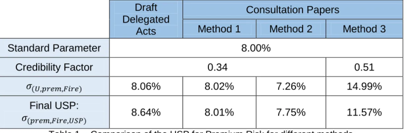
6.3. Results

The results obtained for Premium and Reserve Risk are presented respectively in the following two tables:

Draft Delegated

Acts

Consultation Papers

Method 1 Method 2 Method 3

Standard Parameter 8.00%

Credibility Factor 0.34 0.51

𝜎_{(𝑈,𝑝𝑟𝑒𝑚,𝐹𝑖𝑟𝑒)} 8.06% 8.02% 7.26% 14.99% Final USP:

𝜎(𝑝𝑟𝑒𝑚,𝐹𝑖𝑟𝑒,𝑈𝑆𝑃) 8.64% 8.01% 7.75% 11.57%

Table 1 – Comparison of the USP for Premium Risk for different methods

As can be seen all the Undertaking Specific Parameters for Premium Risk are closer to the Standard Parameter, except the one obtained with method 3. Method 3 produced the higher one, in part due to the fact that the estimate of number of claims a priori is done with a very simple method. As expected comparing methods 1 and 2, the second produced the lower USP.

Draft Delegated Acts Consultation Papers

Method 1 Method 2 Method 1 Method 2 Method 3

Standard Parameter 10.00% Credibility Factor 0.51 1.00 0.51 1.00 𝜎_{(𝑈,𝑟𝑒𝑠,𝐹𝑖𝑟𝑒)} 11.05% 13.34% 10.03% 15.26% 13.34% Final USP: 𝜎_{(𝑟𝑒𝑠,𝐹𝑖𝑟𝑒,𝑈𝑆𝑃)} 11.57% 13.34% 10.02% 15.26% 13.34%

Table 2 – Comparison of the USP for Reserve Risk for different methods

In the reserve risk the USP are again all higher than the Standard Parameter, although the one produce by method 1 is similar. Method 2 of the CP produced a higher standard deviation when compared to method 3 due to the fact that the reserve calculated with the

35

DCL is substantially lower than the one calculated with CL (12.57% lower). The method 1 of the Delegated Acts is the second lower USP.

7. Conclusions and further developments

Despite the absence of final specifications the aim of this work was to compare the Undertaking Specific Parameters for premium and reserve risk presented in the draft specifications of a specific line of business with the parameters of the Standard Formula. When working with USP, an intuitive idea is that the USP would be able to diminish the capital requirements, however for the majority of the methods that did not happen and we obtained USP greater than the standard parameters. In fact, the standard parameters are an average of all insurers and reinsurers in the EU market and so is not realistic to think that all insurers calculating USP will obtain a lower value than the standard ones. Some reasons for the high USP may be the fact that the line of business in question is a relatively small one, and also that in the past years the business is growing which can cause an overestimation. In the beginning of this work, we started to divide the line of business into three different branches: however these branches have proved to be very small and therefore very volatile and the decision to aggregate them in the whole line of business was made.

Despite the higher capital requirements caused by USP in this work, the undertaking must always consider to calculate them in order to get a better assessment of their risks. In the future, possible further developments for this work may be the use of other techniques besides the Chain Ladder method to obtain the reserves and also a deeper analyses of the method presented in the final level 2 documentation.

36

Annexes

Annex 1: Representation of the Standard Formula

Source: Revised Technical Specifications – EIOPA (2012) – page 115 SCR Adj BSCR Market Interest Rate Equity Property Spread Currency Con-centration Counter-cyclical premium Health SLT Health Mortality Longevity Disability Mortality Lapse Expenses Revision CAT Non-SLT Health Premium Reserve Lapse Default Life Mortality Longevity Disability Mortality Lapse Expenses Revision CAT Non-life Premium Reserve Lapse CAT Intang OP

37

Annex 2: Correlation Matrixes

Matrix Corr - Correlation matrix between risks of the Basic Solvency Capital Requirement.

Corr J

Market Default Life Health Non-Life

i Market 1 0.25 0.25 0.25 0.25 Default 0.25 1 0.25 0.25 0.5 Life 0.25 0.25 1 0.25 0 Health 0.25 0.25 0.25 1 0 Non-Life 0.25 0.5 0 0 1

Source: Directive 2009/138/EC – annex IV, point 1

Matrix CorrNL – Correlation matrix between sub-risks of the non-life underwriting risk.

CorrNL NLpr NLlapse NLCAT

NLpr 1 0 0.25

NLlapse 0 1 0

NLCAT 0.25 0 1

38

Matrix CorrS – Correlation matrix between lines of business for premium and reserve risks. CorrS 1 2 3 4 5 6 7 8 9 10 11 12 1: Motor Vehicle Liability 1 0.5 0.5 0.25 0.5 0.25 0.5 0.25 0.5 0.25 0.25 0.25 2: Other Motor 0.5 1 0.25 0.25 0.25 0.25 0.5 0.5 0.5 0.25 0.25 0.25 3: MAT 0.5 0.25 1 0.25 0.25 0.25 0.25 0.5 0.5 0.25 0.5 0.25 4: Fire 0.25 0.25 0.25 1 0.25 0.25 0.25 0.5 0.5 0.25 0.5 0.5 5: General Liability 0.5 0.25 0.25 0.25 1 0.5 0.5 0.25 0.5 0.5 0.25 0.25 6: Credit 0.25 0.25 0.25 0.25 0.5 1 0.5 0.25 0.5 0.5 0.25 0.25 7: Legal Expenses 0.5 0.5 0.25 0.25 0.5 0.5 1 0.25 0.5 0.5 0.25 0.25 8: Assistance 0.25 0.5 0.5 0.5 0.25 0.25 0.25 1 0.5 0.25 0.25 0.5 9: Miscellaneous 0.5 0.5 0.5 0.5 0.5 0.5 0.5 0.5 1 0.25 0.5 0.25 10: Np. Reinsurance (casualty) 0.25 0.25 0.25 0.25 0.5 0.5 0.5 0.25 0.25 1 0.25 0.25 11: Np. Reinsurance (MAT) 0.25 0.25 0.5 0.5 0.25 0.25 0.25 0.25 0.5 0.25 1 0.25 12: Np. Reinsurance (property) 0.25 0.25 0.25 0.5 0.25 0.25 0.25 0.5 0.25 0.25 0.25 1

39

Annex 3: Credibility Factor

Credibility factor for the lines of business Number of

years 5 6 7 8 9 10 11 12 13 14 >14

Credibility

factor 34% 43% 51% 59% 67% 74% 81% 87% 92% 96% 100% Source: Delegated Acts – EIOPA (2014b) – page 401

Credibility factor for the remaining lines of business: Number of

years 5 6 7 8 9 >9

Credibility

factor 34% 51% 67% 81% 92% 100% Source: Delegated Acts – EIOPA (2014b) – page 401/402