For
Jury
Ev
aluation
F
ACULDADE DEE
NGENHARIA DAU
NIVERSIDADE DOP
ORTOEmpirical study of the behavior of
several recommender system methods
on SAPO Videos
Guaicaipuro Alberto Oliveira Neves
Mestrado Integrado em Engenharia Informática e Computação Supervisor: Carlos Manuel Milheiro de Oliveira Pinto Soares
Co-supervisor: Tiago Daniel Sá Cunha
c
Empirical study of the behavior of several recommender
system methods on SAPO Videos
Guaicaipuro Alberto Oliveira Neves
Mestrado Integrado em Engenharia Informática e Computação
Resumo
Nos últimos anos, a internet tornou-se numa ferramenta indispensável para qualquer empresa ou cidadão comum. O que levou à uma enorme quantidade de informações estar disponível aos seus utilizadores. Esta sobrecarga de informação tornou-se num problema urgente que faz com que o utilizador não consiga manter o controle dos seus próprios interesses. Para resolver este problema, os sistemas de recomendação são desenvolvidos para sugerir automaticamente itens que sejam do interesse dos utilizadores.
Existem várias estratégias de recomendação sendo as mais usualmente utilizadas o collab-orative filtering e o content-based filtering. Ainda assim existem ainda muitas outras formas de recomendação das quais podemos identificar: Social based filtering, Social tagging filtering, Knowledge-based filtering, hybrid filtering, context-aware filtering and time-aware filtering.
Esta tese tem como objetivo realizar um estudo empírico sobre recomendação de vídeos no site do Sapo. A motivação para este trabalho foca-se em avaliar qual a melhor estratégia para o problems proposto.
Para realização deste estudo, é necessário fazer um levantamento de diferentes ferramentas de recomendação, recolher e preparar os dados a serem utilizados na plataforma experimental. Para este efeito o RiVaL toolkit é utilizado, de forma a executar diferentes estratégias de ferra-mentas distintas, avaliando-as sempre das mesma forma usando métricas de avaliação que mais se adequarem ao problema.
A avalição deste estudo empírico teve por base três métricas (Precision, RMSE, NDCG), ten-tando encontrar padrões dos resultados das mesmas em diferentes execuções do módulo experi-mental.
Depois do trabalho realizado conclui-se que as filtragens realizadas ao dataset original tem um grande impacto na performance final dos algoritmos. Obtendo-se no geral melhores resultados a nivél de precisão e NDCG e piorando os resultados de RMSE.
Existem três algoritmos que merecem destaque, Item-based usando como similaridade Pear-son’s correlation, que obtém bons resultados na ferramenta Apache Mahout. No que diz respeito ao LensKit as estratégias de Matrix factorization tem sempre boa performance nas diferentes métricas. Pelo lado negativo a similaridade de cosine obtém sempre má performance em ambas ferramentas. No final, conclui-se que mesmo tendo um controlo de como os dados são tratados e avaliados em diferentes ferramentas os seus resultados não são totalmente comparáveis.
Abstract
In the last years, the internet became an indispensable tool for any company or internet user, which led to a huge amount of information being at every internet user’s disposal. This information overload became a pressing problem making the user unable to keep track of his own interests. To solve this issue, recommender systems are developed to automatically suggest items to users that may fit their interests.
The are a numerous amount of different strategies used being the most popular collaborative filtering and content based filtering. Some others can be found in current bibliography about the subject like: 1) Social based filtering, 2) Social tagging filtering, 3) Knowledge-based filtering, 4) hybrid filtering, 5) context-aware filtering and 6)time-aware filtering. This last ones will not be focused in the state of the art because they are not applied in the empirical study.
This thesis aims to do an empirical study regarding recommender systems strategies for the Sapo Videos website. The motivation for this work lays with assessing which is the best strategy for the proposed problem, that leads to finding the best tool and evaluation metrics. There are a lot of different tools and metrics to implement and evaluate this kind of strategies finding the best one will point out that best strategy.
To accomplish this study it will be necessary to survey different recommendation tools, collect and prepare the data to be used on the experimental plataform. For this effect RIVAL toolkit is used allowing the use of different recommendation frameworks and ensuring control over the evaluation process.
The evaluation process used three common metrics (Precision, RMSE, NDCG), leading to patterns in their comparison and in different executions of the experimental module.
The first thing to notice is that the dataset filtrations have a huge impact on the performance, being that for precision and NDCG seems to only improve by increasing the filtering thresholds
In the end, it was concluded that even so the data was handled and evaluated the same way for the different frameworks, the results are not directly compared between them.
Agradecimentos
Gostaria de deixar o meu muito obrigado a todas as pessoas que me acompanharam ao longo do meu percurso académico, e que de algum modo, contríbuiram para a realização da minha dissertação, sendo este um marco importante, agradecer a quem me ajudou a chegar até aqui.
Agradeço ao Prof. Dr. Carlos Soares pela orientação e acompanhamento, pela partilha de conhecimento e pela compreensão durante o longo percurso percorrido na realização desta disser-tação.
Agradeço também ao meu co-orientador e amigo Eng. Tiago Cunha por todo o trabalho, empenho e troca de conhecimentos. Acima de tudo agradeço a disponibilidade e acompanhamento contínuo duranto este ano.
Agradeço bastante a minha mãe pela paciência demostrada, pelos conselhos e pelo apoio prestados para a concretização desta etapa da minha vida.
Agradeço a minha tia pelo trabalho, e pelo empenho que sempre demonstrou num papel de uma excelente segunda mãe.
Agradeço também a todos os professores com quem tive oportunidade conhecer, e com quem aprendi algo para a minha formação futura.
Agora que irei agradecer aos meus amigos, a quem tive oportunidade de me cruzar não só durante a minha vida académica mas tabém fora dela, poupem-me os formalismos.
A vocês a família que escolhi para me acompanhar nestes longos sete anos, a quem conheci nos meus anos enquanto membro da AEFEUP. Aos ditos velhos, Ricardo Martins, Brunho Canhoto e Hugo Carvalho, por todos os ensinamentos e confiança que depositaram em mim.
Aos que comigo entraram e me acompanharam durante todos esses anos, ao quarteto de química, Mimi Mendes, Maria Afonso, Guida Santos e Inês Guimarães, obrigado pela com-panhia, pelos conselhos e pelos jantares quando estava desalojado. Ao Ricardo Rocha, Pedro Kretschmann, Tiago Baldaia e Diogo Moura, obrigado pelo companheirismo, pela ajuda e pelo apoio demonstrado nestes longos anos.
Aos que a seguir vieram e mesmo assim tenho o prazer de ter como amigos, José Pedro Nunes, Rita Magalhães, Bruno Guimarães, João Brochado e especialmente ao Bruno Sousa, por serem excelentes amigos e por toda a ajuda que sempre me prestaram.
Não podia concluir estes agradecimentos sem mais uma vez agradecer individualmente a ti Ricardo Martins, companheiro de todas as horas, porque nem todos os irmãos são de sangue.
A vocês agradeço, Guaicaipuro Neves
“There are two rules for success: 1) Never tell everything you know.”
Contents
Agradecimentos iii 1 Introduction 1 1.1 Overview . . . 1 1.2 Motivation . . . 2 1.3 Goals . . . 2 1.4 Thesis Stucture . . . 2 2 Recommender Systems 4 2.1 Taxonomy . . . 5 2.1.1 Collaborative Filtering . . . 5 2.1.2 Content-Based Filtering . . . 7 2.1.3 Hybrid Filtering . . . 9 2.2 Evaluation . . . 10 2.3 Empirical Studies . . . 12 2.4 Frameworks . . . 13 2.5 Summary . . . 15 3 Experimental Methodology 17 3.1 SAPO Data . . . 17 3.1.1 Data Collecting . . . 17 3.1.2 Data Preparation . . . 193.1.3 Exploratory Data Analysis . . . 20
3.2 Implementation Details . . . 22
3.2.1 RiVaL Toolkit . . . 22
3.2.2 System Architecture . . . 23
4 Analysis and Discussion of Results 25 4.1 Dataset Analysis . . . 25
4.1.1 Original Dataset . . . 25
4.1.2 Video Filtering . . . 27
4.1.3 User Filtering . . . 29
4.2 Discussion and Comparison of Results . . . 30
4.2.1 Discussion . . . 30
4.2.2 Empirical Study Comparison . . . 31
5 Conclusion and Future work 34 5.1 Future Work . . . 35
CONTENTS
6 Result Tables 36
6.1 Video Filtering Dataset . . . 36
6.2 User Filtering Dataset . . . 42
List of Figures
2.1 Websites using Recommender Systems . . . 4
2.2 User-Item rating matrix . . . 5
2.3 Example of features for selection . . . 8
2.4 Different alternatives to combine Content-based and Collaborative Filtering . . . 9
2.5 Recommender System evaluation metrics . . . 11
2.6 Schematic view of the stages followed in an offline evaluation protocol for RS . . 12
3.1 RSS feed from SAPO Videos data . . . 18
3.2 Aspect of final dataset in CSV format (UserId, New VideoID, Rating, Timestamp, Randname) . . . 19
3.3 User distribution in dataset . . . 20
3.4 Video distribution in dataset . . . 21
3.5 RIVAL’s Work flow . . . 22
3.6 Example of RIVAL recommendation configurations . . . 23
3.7 System Architecture . . . 24
4.1 RMSE comparison . . . 32
List of Tables
2.1 Empirical studies . . . 13
2.2 Recommendation frameworks . . . 14
4.1 Mahout Collaborative Filtering Original dataset . . . 26
4.2 Mahout Matrix Factorization Original dataset . . . 26
4.3 LensKit Collaborative Filtering Original dataset . . . 26
4.4 LensKit Matrix Factorization Original dataset . . . 27
4.5 Mahout Collaborative Filtering Videos_1 . . . 27
4.6 Mahout Matrix Factorization Videos_1 . . . 28
4.7 LensKit Collaborative Filtering Videos_1 . . . 28
4.8 LensKit Matrix Factorization Videos_1 . . . 28
4.9 Mahout Collaborative Filtering Users_1 . . . 29
4.10 Mahout Matrix Factorization Users_1 . . . 29
4.11 LensKit Collaborative Filtering Users_1 . . . 30
4.12 LensKit Matrix Factorization Users_1 . . . 30
6.1 Mahout Collaborative Filtering Videos_2 . . . 36
6.2 Mahout Matrix Factorization Videos_2 . . . 36
6.3 LensKit Collaborative Filtering Videos_2 . . . 37
6.4 LensKit Matrix Factorization Videos_2 . . . 37
6.5 Mahout Collaborative Filtering Videos_5 . . . 37
6.6 Mahout Matrix Factorization Videos_5 . . . 37
6.7 LensKit Collaborative Filtering Videos_5 . . . 38
6.8 LensKit Matrix Factorization Videos_5 . . . 38
6.9 Mahout Collaborative Filtering Videos_10 . . . 39
6.10 Mahout Matrix Factorization Videos_10 . . . 39
6.11 LensKit Collaborative Filtering Videos_10 . . . 39
6.12 LensKit Matrix Factorization Videos_10 . . . 39
6.13 Mahout Collaborative Filtering Videos_20 . . . 40
6.14 Mahout Matrix Factorization Videos_20 . . . 40
6.15 LensKit Collaborative Filtering Videos_20 . . . 40
6.16 LensKit Matrix Factorization Videos_20 . . . 40
6.17 Mahout Collaborative Filtering Videos_50 . . . 41
6.18 Mahout Matrix Factorization Videos_50 . . . 41
6.19 LensKit Collaborative Filtering Videos_50 . . . 41
6.20 LensKit Matrix Factorization Videos_50 . . . 41
6.21 Mahout Collaborative Filtering Users_2 . . . 42
LIST OF TABLES
6.23 LensKit Collaborative Filtering Users_2 . . . 43
6.24 LensKit Matrix Factorization Users_2 . . . 43
6.25 Mahout Collaborative Filtering Users_5 . . . 43
6.26 Mahout Matrix Factorization Users_5 . . . 44
6.27 LensKit Collaborative Filtering Users_5 . . . 44
6.28 LensKit Matrix Factorization Users_5 . . . 44
6.29 Mahout Collaborative Filtering Users_10 . . . 44
6.30 Mahout Matrix Factorization Users_10 . . . 45
6.31 LensKit Collaborative Filtering Users_10 . . . 45
6.32 LensKit Matrix Factorization Users_10 . . . 45
6.33 Mahout Collaborative Filtering Users_20 . . . 45
6.34 Mahout Matrix Factorization Users_20 . . . 46
6.35 LensKit Collaborative Filtering Users_20 . . . 46
6.36 LensKit Matrix Factorization Users_20 . . . 46
6.37 Mahout Collaborative Filtering Users_50 . . . 46
6.38 Mahout Matrix Factorization Users_50 . . . 47
6.39 LensKit Collaborative Filtering Users_50 . . . 47
Abbreviations and Symbols
CF Collaborative Filtering CBF Content-based Filtering MF Matrix Factorization
SVD Singular Value Decomposition ALS Alternating Least Squares URL Uniform Resource Locator RMSE Root Mean Square Error
NDCG Normalized Discounted Cumulative Gain CSV Comma Separated Values
Chapter 1
Introduction
2The expansion of the internet and the advent of Web 2.0 allowed users to do more than just access information. Instead of merely reading, a user is invited to comment on published articles, or create 4
a user account or profile on the site. Major features of Web 2.0 include social networking sites, user created Web sites, self-publishing platforms, tagging, and social bookmarking (i.e Youtube, 6
Facebook, Amazon, Blogs). Users can provide the data that is on a Web 2.0 site and exercise some control over it, transforming users from passive consumers to active content producers. 8
The recommendations generated by these systems aim to provide end users with suggestions about products or services that are likely to be of their interest. 10
There are several ways to achieve these recommendations: collaborative filtering methods recommend items that similar users like, while content-based filtering methods recommend items 12
similar to those that the user liked in the past. A combination of different strategies can also be
applied. 14
This has tremendously increased the amount of information that is available to users (Zanardi & Capra, 2008). With this information growth, recommender systems are gaining momentum, 16
because it allows companies to make a more personalized approach for user item interactions.
The combination of personalized recommendations and the pure search and browsing, is a key 18
method for information retrieval nowadays, since it allows users to handle the huge amount of information available in an efficient and satisfying way (Davidson et al.,2010). 20
1.1
Overview
There is a big number of tools that implement the different recommendation strategies, leading to 22
the question of what is the best one to use in the specific problem. It is necessary to study them and try to understand which is better for the task at hand. An empirical study is a way of gaining 24
knowledge regarding this question by means of direct and indirect observation or experience.
The results of such a study must be adequately evaluated. In recommender systems, the most 26
Introduction
(using users to directly evaluate the recommendations, and offline evaluation (using a set of eval-uation metrics for the specific problem). There are numerous amount distinct metrics and each
2
of them evaluated very different aspects of the recommendation (Bobadilla, Ortega, Hernando, & Gutiérrez,2013).
4
1.2
Motivation
The purpose of this thesis is to give Sapo Videos1an idea of what is the best method or methods
6
to make recommendations for their data. These kind of systems give companies like Sapo a huge competitive advantage because it allows its user to find videos they enjoy watching in a easy and
8
direct way, which otherwise the user probably would not find. YouTube for example has a very powerful recommendation system in order to keep users entertained and engaged.
10
For a good use of recommendation system it is imperative that these recommendations are up-dated regularly and reflect a user’s recent activity on the site, consequently these systems increase
12
the number of users, a more importantly their loyalty.
As a scientific contribution this aims to give a comparison on the conclusions obtained by
14
other similar empirical studies and if they apply using the data from Sapo Videos.
It is of the utmost importance that an empirical study is carried as a first step for
recommenda-16
tion system to be created at Sapo Videos. In a world where every minute there are hours of videos uploaded to the internet, this may be an important contribution for Sapo to thrive.
18
1.3
Goals
This thesis aims to do an empirical study of the behavior of different recommendation methods on
20
the Sapo Videos data. This empirical study will need firstly the identification several recommender system methods that are representative of the different strategies.
22
Before the experimental structure implementation it is necessary to collect the data from Sapo Videos and prepare it to run the experiments. For this experimental structure the RiVaL toolkit
24
was selected, because it includes three popular recommendation frameworks (Apache Mahout, LensKit, MyMediaLite).
26
Afterwards, the methods have to be evaluated with the data from Sapo Videos using appropri-ate metrics. The end goal of this thesis is to find patterns in the results obtained, discussing this
28
results and comparing them with other empirical studies.
This will allow the gain of new conclusion of which is the best method for Sapo videos to
30
proceed.
1.4
Thesis Stucture
32
Besides the introduction, these dissertation contains 4 more chapters.
Introduction
In Chapter2, the state of the art regarding recommender systems is described, as well as the most commons strategies of recommendation, how they are evaluated and some empirical studies 2
already done on the subject.
Chapter3, gives us a detailed insight on how the empirical study described in this thesis was 4
conducted, how the data needed was collected and prepared for the recommendation toolkit used. This toolkit is then described, namely explaining how it works and how it fits in the implementation 6
architecture developed.
In chapter 4, the results obtained are presented and discussed. These conclusions are then 8
compared to those obtained in another study, also made with RiVaL toolkit.
Chapter 2
Recommender Systems
2
This transformation of users from passive consumers to active producers of content generated an amount of data online which makes it impossible for the users to keep up with. To deal with this
4
problem, recommender systems arose to automatically suggest items that may interest the user (Bobadilla et al., 2013; Yang, Guo, Liu, & Steck, 2014). Although the roots of recommender
6
systems can be traced back to the extensive work in other scientific areas, recommender systems appeared as an independent research in the mid-1990s (Adomavicius & Tuzhilin,2005;Yang et al.,
8
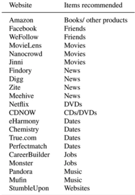
2014). Recommender systems have become extremely common in recent years, and are applied in a variety of applications. The most popular ones are movies, music, news, books, research articles,
10
and products in general, as it is presented in Figure2.1.
Figure 2.1: Websites using Recommender Systems (Lü et al.,2012)
Recommender Systems
Recommender Systems collect information on the preferences of its users for a set of items in an explicit (user’s rating) or implicit form (user’s behaviour) and make use of different types of 2
information to provide its users with predictions and recommendations of items (Bobadilla et al.,
2013). 4
In this chapter it is described the general concept of a recommender systems. We then ex-plain in more detail the most common strategies of recommendation and what type of data, what 6
algorithms are used and how they recommend an item.
The end of the chapter is focused on how recommender systems are evaluated and it is shown 8
some conclusion of empirical studies on the subject.
2.1
Taxonomy
10In this section it will be discussed the most common recommendations taxonomy, the most popular strategies and how they evolved to resolve typical recommendation problems. 12
2.1.1 Collaborative Filtering
Collaborative Filtering works under the assumption that if two users are similar they probably like 14
the same items. The key idea behind collaborative filtering is to use the feedback from each indi-vidual user as a base for recommendations. This feedback can be distinguished between explicit 16
feedback, where the user assigns a rating to an item, or implicit feedback, when for instance the user clicks on a link or sees a video (Yang et al.,2014). 18
Formally collaborative filtering can be represented by: the utility u(c, si) of item s for user c is
estimated based on the utilities u(cj, si) assigned to item s by those users cj∈ C who are “similar” 20
to user c.
In typical collaborative filtering based recommender systems the input data is a collection of 22
user-item interactions. It is usually represented as an U × I user-item rating matrix, such as, un
represents de users and in the number of items as we see in figure2.2(Yang et al.,2014;Sarwar, 24 Karypis, Konstan, & Riedl,2000).
Figure 2.2: User-Item rating matrix (Bobadilla et al.,2013)
Recommender Systems
Furthermore a widely accepted taxonomy divides recommender systems into memory-based and model-based methods. Essentially the former are heuristics that make rating predictions based
2
on the entire collection of previously rated items by the users, whereas the latter use the collection of ratings to learn a model, which is then used to make recommendations (Bobadilla et al.,2013;
4
Yang et al.,2014;Adomavicius & Tuzhilin,2005). The most common memory-based algorithms in collaborative filtering are user-based nearest neighbor and item-based nearest neighbor.
User-6
based and Item-based kNN recommend items for a particular user by, calculating the similarity between users or items respectively using similarity measures. The most common metrics for this
8
type of methods are Pearson’s correlation or Cosine similarity:(Sarwar et al.,2000)
Pearson’s correlation – Similarity between two users u0 and u1, whereas vk and wk, are the 10
vectors of u0X Siand u1X Si. It is measured by calculating:
sim(u0, u1) = ∑ K k=1(vk− v)(wk− w) q ∑Kk=1(vk− v)2∑Kk=1(wk− w)2 (2.1)
Cosine measure – In this case users u0 and u1 are represented as two vectors, the similarity 12
between them is measured by computing the cosine of the angle between them: sim(u0, u1) =
v.w
||v||w|| (2.2)
But it can also be found the use of other similarity measures as part of the list of possible ones
14
to use in these algorithms. As it will be seen the analysis of results some of this may include Tanimoto coefficient and the familiar Euclidean distance.
16
Using the selected similarity measure we produce a neighborhood, for each user or item. User-based nearest neighbor then predicts the missing rating of a user u to an item s with the formula
18 2.3. pred(u, s) = Ru+ ∑n⊂neighbours(u)userSim(u, n).(Rni− Rn) ∑n⊂neighbours(u)userSim(u, n) (2.3) Being Sim the function of similarity used to calculate de similarity between users or items, rui 20
is the rating of the user user u to an item i and ruis the average value of recommendations for user
u.
22
On the other hand Item based nearest neighbor predictions take into account the ratings users gave to similar items, using the equation:2.4.
24
pred(u, s) =∑j∈ratedItems(u)Sim(s, j).Rui ∑j∈ratedItems(u)Sim(s, j)
(2.4) Despite collaborative filtering being a very popular approach it may potentially pose some problems including sparsity, scalability and the cold-start problem. Sparsity is the problem that
26
appears because each user has typically provided only a few ratings and cannot cover the entire spectrum of items. This affects negatively the number of items for which recommendations can
28
Recommender Systems
have used dimensionality reduction techniques. Some reduction methods are based on Matrix Factorization (Bobadilla et al.,2013). Matrix factorization characterizes both items and users by 2
vectors of factors implicit from item ratings of a certain user, being that the major challenge of these methods is computing the mapping of each item and user factor vectors (Koren, Bell, & 4 Volinsky,2009). After this mapping is complete the recommender system can easily estimate the
rating to a given item. 6
Some of the most established techniques for identifying factors is singular value decomposi-tion (SVD). Applying SVD in the collaborative filtering domain requires factoring the user-item 8
rating matrix. Then there was an urge to improve the matrix factorization strategies. To optimize these strategies, the two most used approaches are the Stochastic gradient descent (SGD) and 10
Alternating least squares (ALS)(Koren et al.,2009).
The Scalability problems appear since the computational complexity of these methods grows 12
linearly with the number of users and items. This has a huge impact on typical commercial ap-plications that can grow to several millions user and/or items(Sarwar et al., 2000)(Deshpande 14 & Karypis, 2004). Some solutions appeared like Hadoop and Spark1 for distributed processing, reducing the processing times of Map reduce algorithms. An example is MLI, an application pro- 16
gramming interface designed to address the challenges of building data mining algorithms in a distributed setting.(Sparks & Talwalkar,2013) 18
The cold start problem occurs when it is not possible to make reliable recommendations due to the initial lack of ratings and this problem can be sub-divided in new community, refers to the 20
difficulty when starting up a recommendation system, in obtaining a sufficient amount of data for making reliable recommendations. New item problem, becomes evident when the new items are 22
entered in the recommendation system do not usually have initial ratings, and therefore, they are not likely to be recommended. New user problem, appears since new users have not yet provided 24
any rating in the recommendation system, they cannot receive any personalized recommendations
(Bobadilla et al.,2013). 26
2.1.2 Content-Based Filtering
Content-based filtering makes recommendations based on user choices made in the past, and it 28
follows the principle that items with similar attributes will be rated similarly (Bobadilla et al.,
2013). For example, if a user likes a web page with the words "car", "engine" and "gasoline", the 30
content-based recommender system will recommend pages related to the automotive world.
Content-based filtering has become more important due to the increase of social networks. 32
Recommender systems show a clear trend to allow users to introduce content, such as com-ments, critiques, ratings, opinions and labels as well as to establish social relationship links. 34
(Adomavicius & Tuzhilin,2005) states that content-based recommendation methods, the utility uc,sof the item s for the user c is estimated based on the utilities uc,si assigned by the user c to the 36
items si∈ S that are similar to item s.
Recommender Systems
In a video recommendation application, in order to recommend movies to user u, the content-based filtering recommender system tries to understand the common features among the videos of
2
the user u has rated highly in the past. One problem is that sometimes the item descriptions are unstructured. One common case is when items are represented by documents and it is important
4
to organize the data in such a way that it is possible to conduct the computation of similarities, to address these problems. Researchers have applied data-mining and natural language processing
6
techniques to automate the process of mining features from items as can be seen in Figure2.3
(Dumitru et al.,2011).
8
Figure 2.3: Example of features for selection
After the data is structured it is necessary to make a user profile relatively to the user’s pre-ferred items. There are two main sources of information, a model of the user’s preferences that is
10
basically a description of what types of items interest the user. A history of the user’s interactions with the recommendation system, this interactions can be implicit or explicit(Pazzani & Billsus,
12
2007). Explicit interactions relies on something similar to “like” and “dislike” buttons in the user interface. By using them, the user can state her opinion on the current recommendation. Implicit
14
interactions can for example observe the time the user is actually watching the program (Dumitru et al.,2011).
16
The key purpose for content-based filtering is to determine whether a user will like a specific item. This task is solved traditionally by using heuristic methods or classification algorithms,
18
such us: rule induction, nearest neighbors, decision trees, association rules, linear classifiers, and probabilistic methods (Pazzani & Billsus,2007;Bobadilla et al.,2013).
20
Two of the most important problems for content-based filtering are limited content analysis and overspecialization. The first problem emerges from the difficulty in extracting automated
22
information from some types of content (e.g., images, video, audio and text), which can diminish the quality of the recommendations and introduce a large overhead.
24
The second one refers to the occurrence of users only receiving recommendations for items that are very similar to the items they liked. This means that, users are not receiving recommendations
Recommender Systems
of items they would like but are unknown. Some authors refer this as serendipity (Bobadilla et al.,
2013). 2
2.1.3 Hybrid Filtering
Because of the problems presented above, it is more common to find the combinations of Content- 4
based filtering and Collaborative filtering which are known as Hybrid Filtering. Collaborative filtering solves content-based’s filtering problems because it can function in any domain, it is less 6
affected by overspecialization and it acquires feedback from users. Content-based filtering adds the following qualities to Collaborative Filtering, improvement to the quality of the predictions 8
(because they are calculated with more information), and reduced impact from the cold-start and sparsity problems. A proper hybrid recommendation algorithm can be devised and applied to fit 10
the type of information available in a specific domain (Jeong,2010).
Content-Based and Collaborative Filtering can be combined in different ways. The different 12
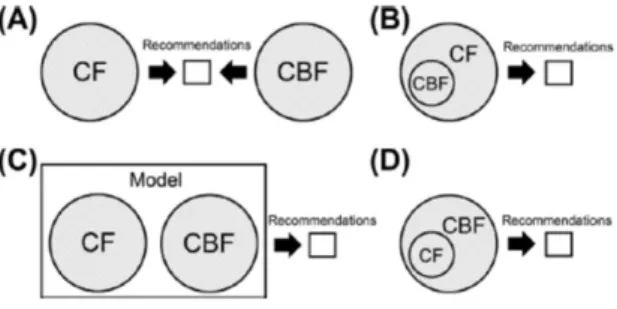
alternatives as shown in Figure2.4(Bobadilla et al.,2013). There are several different approaches to hybridization. It is possible to (A) implement collaborative and content-based methods sep- 14
arately and combine their predictions, (B) incorporate some content-based characteristics into a collaborative approach, (C) build a general unifying model that incorporates both content-based 16
and collaborative characteristics and (D) include some collaborative characteristics into a content-based approach. The most challenging way is to construct a unified model (Bobadilla et al.,2013; 18 Christakou, Vrettos, & Stafylopatis,2007).
Figure 2.4: Different alternatives to combine Content-based and Collaborative Filtering (Bobadilla et al.,2013)
For example, (Melville, Mooney, & Nagarajan,2002) uses hybridization in the movie recom- 20
mendation domain. The basic approach uses content-based predictions to convert a sparse user ratings matrix into a full ratings matrix and then uses CF to provide recommendations. The re- 22
search developed by (Christakou et al.,2007) considered a combination of CF and CBF, as the two approaches are proved to be almost complementary. A user evaluates films that he/she has seen 24
on a discrete scale. This information allows the system to learn the preferences of the user and subsequently, construct the user’s profile. We take into consideration two elements: the content of 26
Recommender Systems
films that individuals have already seen and the films that persons with similar preferences have liked, as a result, they enhance both performance and reliability.
2
(Jeong,2010) proposes a hybrid algorithm combining a modified Pearson’s correlation coefficient-based collaborative filtering and distance-to-boundary (DTB) coefficient-based content-coefficient-based filtering. The
4
study focused on developing a hybrid approach that suggests a high-quality recommendation method for a tremendous volume of data. The results indicated that this hybrid model performed
6
better than the pure recommender system and by integrating both CB and CF strategies, the per-sonalization engine provided a powerful recommendation solution.
8
Lastly, (Saveski & Mantrach,2014) introduced a new method for Email Recipient recommen-dation that combines the content and collaborative information in a unified matrix factorization
10
framework while exploiting the local geometrical structure of the data.
2.2
Evaluation
12
With the growth of the recommender systems research, assessing the performance of recommender systems became an important factor of success and more importantly, a way to gain a better
under-14
standing of recommender system behavior. This leads to an increase of evaluation approaches in an effort to determine the best approach and their individual strengths and weaknesses. Evaluating
16
recommender systems and their algorithms can be very difficult for two reasons. First, different algorithms perform differently on different data sets. Secondly, the goals for which an evaluation
18
is performed may be very different (Herlocker, Konstan, Terveen, & Riedl,2004).
(Beel, Genzmehr, Langer, Nürnberger, & Gipp,2013) state that finding the best recommender
20
systems methods is not simple, and separates evaluation into three main methods: user studies, online evaluation and offline evaluation. User studies works on the basis that users explicitly rate
22
recommendations generated by different algorithms, basically they quantify the user’s satisfaction with the recommendations. In addition to this, user studies ask the user to rate a single aspect of
24
the recommender system, but this method is not frequently used.
In online evaluation, recommendations are shown to real users of the system during their
26
session. In this method users do not rate recommendations. Instead recommender systems capture how often the user accepts a recommendation. This acceptance is normally measured in
click-28
through rate (CTR), which measures the ratio of clicks to impressions of an online item. The online method serves to implicitly measure the user’s satisfaction.
30
Offline evaluations operates using datasets containing past users behavior from which some information has been removed (i.e the information removed can be the rating a user gave to an
32
item). Afterwards, results are obtained by analyzing their ability to recommend/predict this miss-ing information. (Campos, Díez, & Cantador, 2013; Herlocker et al., 2004;Beel et al., 2013).
34
This process can be seen in Figure2.6, basically the dataset is divided into training and testing datasets. The training set is sent to the recommendation model to train it on how the users will rate
36
Recommender Systems
or that have been removed for this purpose. To assess the performance of the recommendations the evaluations metrics are applied on the recommendations generated2.5. 2
This means that we must split the data into training and testing datasets. The main differences are that the evaluation metrics must suit the problem at hand and one must split the test data into 4
hidden and observable instances.
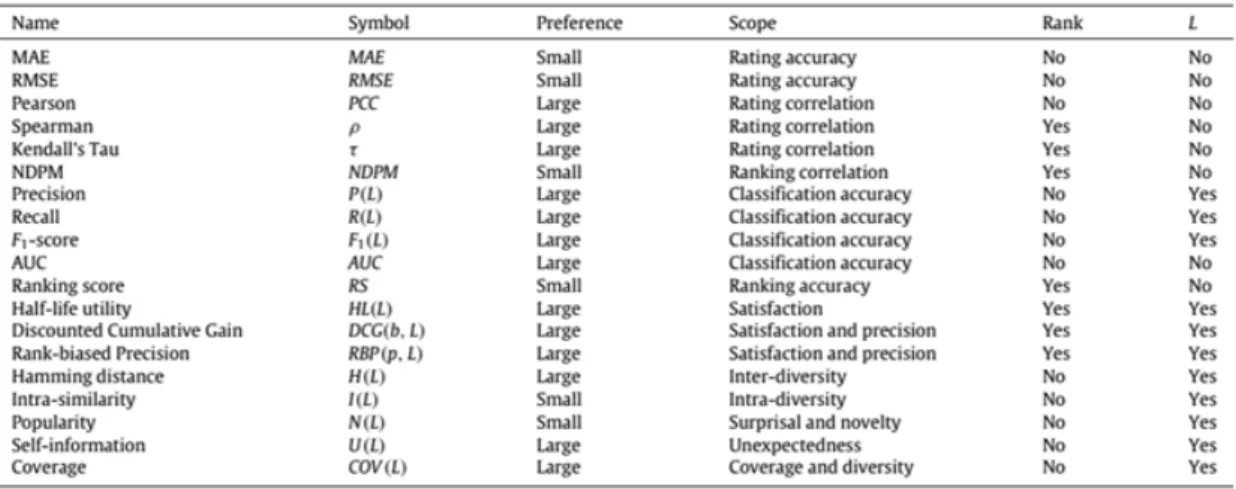
Figure 2.5: Recommender System evaluation metrics (Lü et al.,2012)
In order to evaluate Recommender Systems, several metrics are proposed (Bobadilla et al., 6 2013;Lü et al.,2012). Figure2.5shows some of the most common evaluation metrics and on what type of dataset they are most suited, as for on which aspect of the recommendation it evaluates. 8
Here, we focus on three main evaluation strategies. Firstly RMSE is a typically metric used to measure the error on the rating predictions and it is calculated by (Herlocker et al.,2004;Jiang, 10 Liu, Tang, & Liu,2011):
RMSE= s
∑Nk=1(pui− rui)2
N (2.5)
Precision and NDCG on the other hand are used for classification accuracy measurement, pre- 12
cision is the fraction of retrieved documents that are relevant, this is the fraction of true positives. The formula used to calculate precision is (Gunawardana & Shani,2009): 14
Precision= T P
T P+ FP (2.6)
NDCG is the ratio between the DCG and the IDCG, which is the maximum possible gain value for user u (Baltrunas, Makcinskas, & Ricci,2010), it measures the usefulness, or gain, of an item 16
based on its position in the result list. It is calculated with:
NDCGuk= DCG
u k
Recommender Systems
Figure 2.6: Schematic view of the stages followed in an offline evaluation protocol for RS (Campos et al.,2013)
2.3
Empirical Studies
Table2.1presents some empirical studies on the area of recommender systems, which have to be
2
analyzed to find the main conclusion of the experiments.
In this case it is analyzed which datasets were used, which algorithms for recommendations
4
they tried and some of the main conclusion their drew from they study.
(Adomavicius & Zhang,2012) tried to understand the stability of the most common
collabo-6
rative filtering algorithms.
(Ekstrand et al.,2014) used online evaluation metrics trying to prove that, offline metrics fail
8
to capture much of what will impact the user’s recommendation experience.
The only empirical studies found that used content-based filtering was (Cantador, Bellogín, & 10
Vallet, 2010), that compared three methods of content-based filtering (FIDF Cosine-based Sim-ilarity, BM25-based Similarity and BM25 Cosine-based Similarity), on two different data types
12
(Delicious and Last.fm).
As it is shown most of the studies experiment only with collaborative filtering, this may be due
14
to the fact that is still on of the most used methods for recommendations and there is huge amount of public tools that implement collaborative filtering algorithms.
Recommender Systems
Table 2.1: Empirical studies
Paper Data types Algorithms Main Conclusions (Adomavicius & Zhang, 2012) Movielens, Joker Item Average; User Average; User-ItemAverage; Item-based kNN; User-based kNN; Matrix Factoriza-tion (SVD)
Model-based techniques are more stable than memory-based collaborative filtering heuristics; Normalizing rating data before applying any al-gorithms not only improves accuracy for all rec-ommendation algorithms, but also plays a critical role in improving their stability;
(Ekstrand, Harper, Willemsen, & Konstan, 2014) Movielens Item-based CF; User-based CF; Matrix Factoriza-tion (SVD)
Item-based CF and SVD performed very simi-larly, with users preferring them in roughly equal measure;
Offline metrics fail to capture much of what will impact the user’s experience with a recommender system.
(Said & Bel-logín,2014) MovieLens, Yelp User-based CF; Item-based CF; Matrix factoriza-tion(SVD)
Different frameworks implement and evaluate the same algorithms in distinct ways
leading to the relative performance of two or more algorithms evaluated under different con-ditions becoming essentially meaningless.; (Vargas & Castells, 2011) Delicious, Last.fm TF-IDF Cosine-based Similarity; BM25-based Simi-larity; BM25 Cosine-based Similarity
In general,the models focused on user profiles outperformed the models oriented to item pro-files;
Regarding cosine-based models, by performing a weighting scheme that exploits the whole folk-sonomy, clearly enhance the classic frequency profile representation;
2.4
Frameworks
Table2.2represents a list of public frameworks that implement several recommendations strategies 2
and methods. As it is shown all the frameworks implement only collaborative filtering strategies. This is because collaborative filtering is still the most used method of recommendation. 4
There is a tendency for the most recent frameworks to implement matrix factorization algo-rithms, since it attenuates some of the cold start and sparsity problems that the base collaborative 6
filtering algorithms have.
We could not find any framework that implements content-based methods. This may be caused 8
by the fact that most Content-based filtering techniques use traditionally text mining or classifi-cation algorithms with a vector space model strategy (Pazzani & Billsus,2007;Bobadilla et al., 10 2013).
This empirical study is focused on the two different frameworks that will be used: Apache 12
Mahout10, is a project of the Apache Software Foundation focused primarily in the areas of
Recommender Systems
Table 2.2: Recommendation frameworks
Name Strategies Algorithms Datasets Evaluation Metrics LensKit2 Collaborative Filtering User/Item-based CF;Matrix Factor-ization MovieLens 100K
normalized discounted cumula-tive gain; actual length of the top-N list PREA3 Collaborative Filtering User/item-based CF;Slope One;Matrix Factor-ization
N/A Root of the Mean Square Error (RMSE);Mean Ab-solute Error (MAE); Nor-malized Mean Absolute Error (NMAE);Asymmetric Measures; Half-Life Utility (HLU);Normalized Discounted Cumulative Gain (NDCG) Duine4 Collaborative Filtering User-based kNN MovieLens 100K
Root of the Mean Square Error (RMSE); Mean Absolute Error (MAE); MyMediaLite 5 Collaborative Filtering User/Item based CF MovieLens 1M/10M
Mean Absolute Error (MAE); Root of the Mean Square Error (RMSE);Area Under Curve(AUC); MAP; Neg-ative Discount Comulative Gain(NDCG) Crab6 Collaborative Filtering User/Item based CF N/A Precision;Recall Apache Mahout7 Collaborative Filtering User/Item based CF; Matrix Fac-torization(SVD, ALS)
N/A Average Absolute Difference Er-ror ( AADE); Root of the Mean Square Error (RMSE)
SVDFeature 8 Collaborative Filtering Matrix Factoriza-tion (SVD)
N/A Root of the Mean Square Error (RMSE) PredictionIO 9 Collaborative Filtering Matrix Factoriza-tion (SVD, ALS, PCA)
Recommender Systems
orative filtering, clustering and classification. LensKit11, is a free open source software developed primarily by researchers at Texas State University and GroupLens Research at the University of 2
Minnesota.
2.5
Summary
4This chapter focus on recommender systems, the most used recommendation strategies, how this systems performance is evaluated, other empirical studies on the subject and existing recommen- 6
dation frameworks. Collaborative filtering is the most commonly used strategy and it works on the assumption that if two users are similar they probably like the same items. It used the feedback of 8
each individual user as a basis for recommendations. The feedback can be distinguished into two different categories implicit and explicit feedback. The first algorithms to appear to achieve rec- 10
ommendations where Item/User-based kNN. They calculate the similarity between items or users, using similarity measures (i.e Pearson’s correlation, Cosine similarity). Although this strategy 12
possess problems like scalability the cold start problem.
To resolve these problems other strategy is presented. Content-based filtering, it makes recomme-14
dations based on the choices that the user made in the past. In order to recommend items to and user, the content-based filtering strategy tries to understand the common features among the items 16
that the user rated highly in the past. After this data is structured it is necessary to make the users profile relatively to the user’s preferred items. The key purpose for content-based filtering is to 18
determine whether a user will like a specific item. This task is solved traditionally by using heuris-tic methods or classification algorithms, such us: rule induction, nearest neighbors, decision trees, 20
association rules, linear classifiers, and probabilistic methods.
A combination of the strategies present above is also possible, it is known as hybrid filtering. 22
This type of strategy emerged in a urge diminish the problems other recommendation strategies. Assessing the performance of recommender systems became an important factor of success 24
and more importantly, a way to gain a better understanding of recommender system behavior. This leads to an increase of evaluation approaches. These evaluation approaches can be divided into two 26
categories. Online evaluation, in which recommendations are shown to real users of the system during their session. In this method users do not rate recommendations. Instead recommender 28
systems capture how often the user accepts a recommendation.
Whereas in offline evaluation methods operates using datasets containing past users behavior 30
from which some information has been removed. Afterwards, results are obtained by analyzing their ability to recommend/predict this missing information. 32
Analyzing other empirical studies made in the field of recommender systems, we try to un-derstand what are the main findings other authors take so they can be later compared to the ones 34
made in this work.
Recommender Systems
To the success of this empirical study it is important to understand which recommendation frameworks are most used. From this frameworks it is analyzed what strategies are implemented
2
Chapter 3
Experimental Methodology
2This chapter describes the whole experimental procedure needed to run the experiments. The process has several steps that are described in more detail in the sections bellow. 4
3.1
SAPO Data
This section describes in full detail the first step in this empirical study, specifically how the 6
data was collected and prepared for the experiments. It explains how the data was collected and
processed from the SAPO servers. 8
The data preparation subsection characterizes how the data had to be altered so it would be accepted experimental module and followed the premise that should be handled the same way for 10
the different frameworks.
3.1.1 Data Collecting 12
The data was collected through a RSS feed provided by SAPO. To access it, it was necessary to set up a VPN to the Portugal Telecom intranet. 14
Figure3.1shows the aspect of the raw data stored for user-video interactions. It is important to notice that the data feed provided only keeps stored the data from the last three days of interactions. 16
This limitation has the effect of only providing on average 1000 observations, so it was necessary to develop a solution that collected the data of long periods of time. Storing this three days of 18
interactions of data in a database at a time to get a final dataset with enough observations to run
the experiment. 20
We developed a Python script running on a Linux virtual machine using crontab to run once everyday storing only the new interactions. The script connected to the VPN and run through the 22
feed comparing all the interactions present avoiding collecting duplicate information.
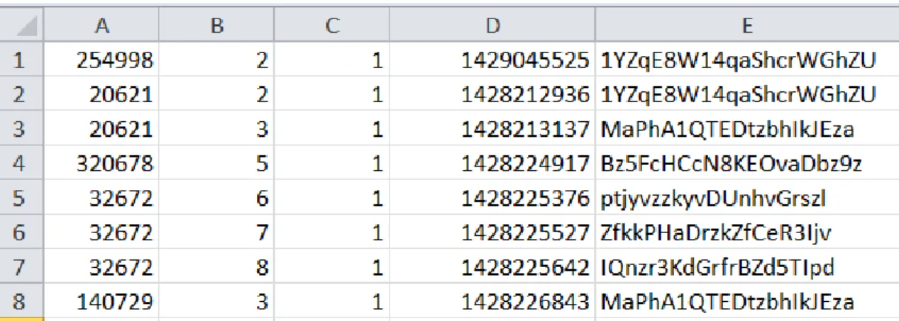
As it can be seen on figure3.1, the information provided is an integer variable userid when 0 24
the user is not a registered user, a string randname as figure it is an unique string the appears on the end of the video URL and the full date when the user saw the video. 26
Experimental Methodology
Experimental Methodology
whenever a user that is not registered or is not logged in the website watches a video, the userid variable appears as 0. As this users can not be used for recommendation this potentially deceases 2
the quality of the data collected as they have to be removed from the dataset.
3.1.2 Data Preparation 4
In this section it will be explained the improvements to the raw data, for example the users that were not registered while watching the videos need to be cut from the final dataset. As it will be 6
explained in full detail, in the experimental methodology section some more changes needed to be made to the final dataset for it to run through the experimental structure already implemented, 8
RiVaL toolkit3.2.
RiVal toolkit was chosen to ensure the data was prepared, handled and evaluated in the same 10
way, regardless of the method, algorithm or framework chosen. Some of the things to take into account for the dataset to run through RiVaL are that firstly as mentioned already the data collected 12
was only implicit and RiVaL handled only explicit datasets in CSV format, making it impossible to use the data collected without changes. The item identification, in this case the randname, had 14
to be a long variable and finally instead of a viewing date it was needed a timestamp instead.
The solution found was to build a new Python script that loaded the data from the database, 16
handled these changes and saved that data on a csv file and when saving to CSV. Since we are working with implicit feedback(i.e user views), we introduced a new column with the number 1 18
on every line. Using Python direct conversion from full date directly to timestamp one problem
was resolved. 20
Now the biggest issue was converting a randname variable to a long one. The key to solving this problem was to create an hash map that for every new line it would search the hash map to 22
see if it was a new randname, in other words a new video. If it was it would add it to the hash map incrementing a new ID. If it already existed on the hash map it would give the new line the ID of 24
the first time the randname appeared. The outcome is visible on Figure3.2.
Figure 3.2: Aspect of final dataset in CSV format (UserId, New VideoID, Rating, Timestamp, Randname)
Experimental Methodology
3.1.3 Exploratory Data Analysis
In this subsection it will be presented an analysis of the quality of the data as for some general
2
statistics about it. The final dataset collected after the unregistered users had a total of 15939 observations, this is user-video interactions.
4
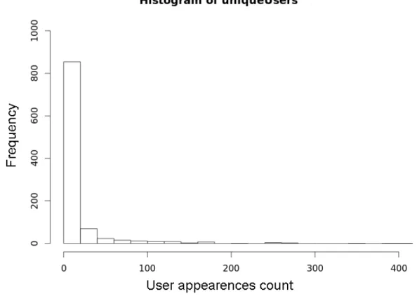
Of this it can be found 1008 unique users and 5880 unique videos the compose the total number of interactions. Observing below on figure3.3, about the user interactions, the histogram presents
6
the distribution of this users relating the number of interactions made present on the dataset. For example it can be seen that more than 800 users watched between 0 and less than 20 videos, and
8
normally it is only between 0 and 5.
For the videos figure3.4gives some insights on the video distribution through the data. As it
10
can be seen the for videos the distribution is even worse, showing that almost all the videos only are watched between 0 and less then 5 times. In conclusion making the user-item rating matrix for
12
the data really sparse, being approximately 0.269
To resolve this problem the dataset was filtered trying to improve the global results. The
14
process in which the data was filtered is explained in the next chapter4.
Experimental Methodology
Experimental Methodology
3.2
Implementation Details
This section describes with great detail the whole experimental structure. Starting how RiVaL
2
toolkit3.2.1works and ensured a fine-grained control over the evaluation process.
The final subsection will explain full process behind the total implementation from the data
4
collecting to the final results.
3.2.1 RiVaL Toolkit
6
The best solution found to accomplish this empirical study and the objectives proposed on Chapter
2was RiVaL toolkit, an open source program developed in Java that allows a subtle control of the
8
complete evaluation process (Said & Bellogín, 2014). RiVaL has integrated three main recom-mendation frameworks (Apache Mahout, LensKit and MyMediaLite), although in this empirical
10
study we considered only two, Apache Mahout nad LensKit. The reason for leaving MyMediaLite out is because the version offered for download on the official website1did not had MyMediaLite
12
available for use. Being that the documentation about RiVaL was weak not allowing understanding on why MyMediaLite was missing.
14
The recommendation process for RIVAL can be defined in four stages, i) data splitting; ii) item recommendation; iii) candidate item generation; iv) performance measurement. Of this four
16
stages only three are performed by RiVaL, since it is not a recommendation framework. Step (iii) is not performed by RiVal, but can be performed by any of the three integrated frameworks
18
(Mahout and LensKit).
Figure 3.5: RIVAL’s Work flow
Experimental Methodology
In this case, steps (i), (iii), and (iv) are performed in the toolkit. As for step (ii) the preferred recommendation framework is given the data splits generated in the previous step and the recom- 2
mendations produced by the framework are then given as input to step (iii) of the stages. Figure
3.5illustrates RiVal’s four stages. 4
To execute RiVaL, the evaluation selected, the algorithms, and the specific framework to use
are specified in property files. 6
The example in Figure3.6shows the a configuration of RIVAL for the recommendation step executing an User-Based algorithm using cosine similarity with a neighborhood size of 50 of the 8
LensKit recommendation framework.
Figure 3.6: Example of RIVAL recommendation configurations
RiVal toolkit had to suffer a set of changes for the Sapo dataset to run, never compromising 10
the normal functioning of the work flow. This changes were mainly because RiVal was developed and tested with good datasets, this means no sparsity problems and always a good number of ob- 12
servations, believing that for every user on the dataset their would be a possible recommendation. This led to, when running experiments, RiVaL could not handle users without possible recom- 14
mendations and stopped running throwing exceptions errors. In the recommendation step it was added different conditional clauses to validate if the user had possible item recommendation, only 16
then proceeding to the next step.
After RiVaL was running correctly for our data, it was needed to find out out algorithms 18
would run for the distinct frameworks. For Apache Mahout the GenericItemBased (Item Based Knn), GenericUserBased (User Based Knn) with different similarity measures (Pearson’s Corre- 20
lation, Cosine Similarity, Tanimoto Coefficient and Spearman Rank). It also implemented Matrix Factorization types with distinct factorization types( FunkSVD, ALSW, Plus Plus factorizer and 22
Rating SGD).
LensKit on the other hand has a fewer number of available algorithms running ItemItemScorer 24
(Item Based Knn), UserUserScorer (User Based Knn) with Spearman Rank, Cosine similarity and Pearson’s correlation as similarity measures. 26
3.2.2 System Architecture
To best explain the implementation system, figure3.7illustrates all the stages. The start of this 28
Experimental Methodology
Detailed explanation on how this how made can be found on3.1.1subsection.
This collected data was then stored in a database. The next step of the implementation was
2
preparing the data and storing it on CSV file (more details on this step are established in3.1.2). From this final dataset, some new datasets were created. The idea behind this new datasets and
4
their explanation are explained on chapter4.
The final stage in the all process was the experimentation process. In this stage all the different
6
datasets, were submitted to RiVaL toolkit, subsection3.2.1, and the evaluation results stored in the database for further processing.
8
Chapter 4
Analysis and Discussion of Results
2This chapter focus on the results obtained, it will be presented the result tables highlighting in green the best result and in red the worst result for each of the different metrics and frameworks in 4
the different datasets. Afterwards conclusions are drawn from the results and why those happened.
4.1
Dataset Analysis
6In the context of obtaining better results and producing a more in depth empirical study, ten dif-ferent datasets were created from the original one. Because of the sparsity in data of the original 8
dataset the results obtained were not satisfactory. These new datasets were created by filtering the original by video, selecting just the videos that had more than a certain number of visualizations, 10
and by User, choosing users that had more than a certain number of videos seen. The selected thresholds were one, two, five, ten, twenty and fifty for both users and videos. These datasets are 12
labeled as video_1 through video_50 for video filtering and user_1 through user user_50 for user
filtering. 14
Another evaluation regarded was the variation of the distinct initial algorithm parameters like neighborhood size and the number of factors in the SVD strategies, in order to study their effects 16
in the overall performance.
The whole empirical study was developed using three main strategies: User Based CF, Item 18
Based CF and Matrix Factorization. Furthermore, different similarity classes and factorizer types were used. It is important to note that from the two frameworks available on RiVaL, Apache 20
Mahout seems more extensive in their selection of strategies and algorithms when compared to
LensKit. 22
The next sections present the results obtained using all these strategies and have been divided in, results of the original, video filtering and user filtering datasets. 24
4.1.1 Original Dataset
The tables presented below show the results for the different algorithms of the distinct frameworks. 26
Analysis and Discussion of Results
groups, both precision and NDCG are used to directly find a list of item to recommend,as a clas-sification accuracy metric. RMSE on the other hand is used to predict the rating the a user would
2
give to a specific item, a rating accuracy metric.
Table 4.1: Mahout Collaborative Filtering Original dataset
Algorithm NDCG RMSE Precision NBsize Similarity Class GenericItemBased 0,0240347 14,12554848 0,003645686 50 Tanimoto Coefficient GenericItemBased 0,021813772 14,12555919 0,002123459 50 Euclidean Distance GenericItemBased 0,021251396 14,12877938 0,002054042 50 Cosine Similarity GenericItemBased 0,081575895 19,3978057 0,026406879 50 Pearson’s Correlation GenericUserBased 0,113550369 15,38540189 0,023660826 50 TanimotoCoefficient GenericUserBased 0,105711383 16,18242996 0,015641249 50 Cosine Similarity GenericUserBased 0,089444303 17,58941012 0,019419683 50 Euclidean Distance GenericUserBased 0,131209389 19,48957225 0,032576487 50 Pearson’s Correlation
Table 4.2: Mahout Matrix Factorization Original dataset
Algorithm NDCG RMSE Precision Factorizer Type Iteractions Factors SVD 0,132614237 13,08272318 0,021578258 ALSWR 50 10 SVD 0,125891765 13,0947511 0,02134621 FunkSVD 50 10 SVD 0,123367101 13,03957183 0,02127789 SVDPlusPlus 50 10 SVD 0,075635674 13,17950689 0,013553344 RatingSGD 50 10 SVD 0,135204589 13,09583287 0,021243526 FunkSVD 50 30 SVD 0,132685476 13,09829961 0,021459288 RatingSGD 50 30 SVD 0,135005957 13,09281137 0,021653886 SVDPlusPlus 50 30 SVD 0,136016267 13,12582943 0,021359499 ALSWR 50 30 SVD 0,139377297 13,10819402 0,021236987 FunkSVD 50 50 SVD 0,137198693 13,13950122 0,022549697 RatingSGD 50 50 SVD 0,136445361 13,12344064 0,022443315 SVDPlusPlus 50 50 SVD 0,138968716 13,13464736 0,021567416 ALSWR 50 50
Table 4.3: LensKit Collaborative Filtering Original dataset
Algorithm NDCG RMSE Precison Nbsize Similarity Class UserUserScorer 0,052756987 13,39676723 0,007624473 50-150 Pearson’s Correlation UserUserScorer 0,042849141 13,2675676 0,007568793 50-150 Cosine Similarity ItemItemScorer 0,012243574 13,29499233 0,000612559 50-150 Cosine Similarity ItemItemScorer 0,049213951 18,58679494 0,011486631 50-150 Spearman Rank ItemItemScorer 0,061317066 17,95627876 0,011355201 50-150 Pearson’s
The first observation found after analyzing the results from the original dataset, is that the
4
change in the initial parameters in the generic collaborative filtering techniques, did not change the outcome of the results. Only in the matrix factorization strategies, changing the parameters altered
6
Analysis and Discussion of Results
Table 4.4: LensKit Matrix Factorization Original dataset
Algorithm NDCG RMSE Precision Factorizer Type Iteractions Factors FunkSVD 0,062440759 14,14141109 0,009459459 FunkSVD 50 50 FunkSVD 0,099069374 14,16353719 0,011238299 FunkSVD 50 30 FunkSVD 0,134704152 14,1786524 0,012453622 FunkSVD 50 10
of the algorithms. On the other hand, Apache Mahout behavior is not stable, resulting in the fact that sometimes the increase of factor improves the algorithms results and sometimes it doesn’t. 2
Generally it can be seen that the best strategy for recommendation in the original dataset both for Apache Mahout and LensKit is based on matrix factorization. The type of factorization though 4
is not unanimous being that FunkSVD and ALS obtain the best results.
On the negative side, Item Based methods combined with cosine similarity measures rank last 6
for the two frameworks on almost every metric evaluated.
4.1.2 Video Filtering 8
The tables in this subsection show the results for the video filtering datasets, as the number of user-item interactions and the sparsity are reduced their results will be presented individually. 10
Table 4.5: Mahout Collaborative Filtering Videos_1
Algorithm NDCG RMSE Precision NBSize Similiraty Class GenericItemBased 0,0212513962 14,2679383015 0,0020840416 50 Cosine Similarity GenericItemBased 0,0815758948 19,5728241970 0,0294068786 50 Pearson’s Correlation GenericItemBased 0,0218137720 14,2622365919 0,0022159516 50 Euclidean Distance GenericItemBased 0,0240346996 14,2070184848 0,0036567621 50 Tanimoto Coefficient GenericUserBased 0,1312093894 19,9713895723 0,0354865192 50 Pearson’s Correlation GenericUserBased 0,1057113827 16,2785506073 0,0177412491 50 Cosine Similarity GenericUserBased 0,0894443033 17,7010744101 0,0194196829 50 Euclidean Distance GenericUserBased 0,1135503686 15,6128852002 0,0246608263 50 Tanimoto Coefficient
Some brief conclusion, that will be discussed more thorough in the next section, can be taken after all this results. Firstly it can be seen, as in the original dataset, that the initial parameters 12
variation only affects the matrix factorization strategies.
Still on this subject it is to notice that the variation of the number of factors in the LensKit 14
framework for the matrix factorization algorithms tends to almost always improve the performance
in the evaluation metrics. 16
This does not happen frequently on the Apache Mahout framework. Usually the increase of the number of factors does not work in favor of better recommendations. 18
For Apache Mahout framework the combination of Item Based strategy with the pearson’s correlation strategy seems to be the best in terms of precision, and the SVD recommendation 20
strategy in NDCG and RMSE, although here the factorization type seems to change a bit in which
Analysis and Discussion of Results
Table 4.6: Mahout Matrix Factorization Videos_1
Algorithm NDCG RMSE Precision Factorizer Iteractions Factors SVD 0,125891765 13,1419368 0,021478541 FunkSVD 50 10 SVD 0,075635674 13,26686894 0,015185873 RatingSGD 50 10 SVD 0,123367101 13,14669053 0,021563982 SVDPlusPlus 50 10 SVD 0,132614237 13,13637859 0,021814113 ALSWR 50 10 SVD 0,1352045893 13,1487615329 0,0238278226 FunkSVD 50 30 SVD 0,1326854755 13,1615260596 0,0227379193 RatingSGD 50 30 SVD 0,1350059568 13,1527947137 0,0226538857 SVDPlusPlus 50 30 SVD 0,1360162669 13,1557500431 0,0220673395 ALSWR 50 30 SVD 0,1393772968 13,1521255096 0,0235751587 FunkSVD 50 50 SVD 0,1371986929 13,1519711218 0,0234919697 RatingSGD 50 50 SVD 0,1364453611 13,1599653600 0,0232401503 SVDPlusPlus 50 50 SVD 0,1389687157 13,1551377364 0,0232415579 ALSWR 50 50
Table 4.7: LensKit Collaborative Filtering Videos_1
Algorithm NDCG RMSE Precison Nbsize Similarity Class UserUserScorer 0,013346787 13,13546895 0,007647289 50 Cosine Similarity UserUserScorer 0,052756987 13,39676723 0,007544726 50 Pearson’s Correlation ItemItemScorer 0,061317066 17,95627876 0,013383565 50 Pearson’s Correlation ItemItemScorer 0,013297403 13,44419579 7,55E-04 50 Cosine Similarity ItemItemScorer 0,049213951 18,58679494 0,011486631 50 Spearman Rank
Table 4.8: LensKit Matrix Factorization Videos_1
Algorithm NDCG RMSE Precison Factorizer Iteractions Factors SVD 0,062440759 14,18221109 0,009459459 FunkSVD 50 50 SVD 0,099069374 14,18344997 0,01518283 FunkSVD 50 30 SVD 0,134704152 14,1956524 0,016216216 FunkSVD 50 10
Analysis and Discussion of Results
On the other hand in the LensKit framework it is not so easy to find the best approach for each individual evaluation metric. It can be said that Item based strategy with cosine similary is a bad 2
strategy to obtain a good precision, and Matrix factorization strategy is a good all around strategy
for this framework. 4
In general it is clear that for video filtration datasets types Item based strategies are a good way to go, this is an expected result because the number of sparse elements is reduced. 6
4.1.3 User Filtering
This subsection presents the results of how the different strategies and algorithms behaved in the 8
user filtering datasets. The evaluation metrics used are the same as in the other analysis. Table 4.9: Mahout Collaborative Filtering Users_1
Algorithm NDCG RMSE Precison Nbsize Similarity Class GenericItemBased 0,017175921 16,01310287 0,001278781 50 Cosine Similarity GenericItemBased 0,077697845 20,48474437 0,026948669 50 Pearson’s Correlation GenericItemBased 0,01658242 16,0083438 0,001533883 50 Euclidean Distance GenericItemBased 0,024032787 15,97350116 0,002174908 50 Tanimoto Coefficient GenericUserBased 0,193427039 21,80282736 0,107653061 50 Pearson’s Correlation GenericUserBased 0,077978159 18,84034312 0,012044316 50 Cosine Similarity GenericUserBased 0,066654683 16,17781762 0,014621505 50 Euclidean Distance GenericUserBased 0,103787542 16,37209262 0,024934999 50 Tanimoto Coefficient
Table 4.10: Mahout Matrix Factorization Users_1
Algorithm NDCG RMSE Precison Factorizer Iteractions Factors SVD 0,108213086 14,91851637 0,020230408 FunkSVD 50 10 SVD 0,06325301 15,03543943 0,014700144 RatingSGD 50 10 SVD 0,10382793 14,92124018 0,020313637 SVDPlusPlus 50 10 SVD 0,106385091 14,91754256 0,020393382 ALSWR 50 10 SVD 0,107423826 14,9254806 0,021198959 FunkSVD 50 30 SVD 0,104560149 14,91946073 0,020953918 RatingSGD 50 30 SVD 0,106339582 14,91554964 0,021517939 SVDPlusPlus 50 30 SVD 0,104123463 14,92665467 0,020394543 ALSWR 50 30 SVD 0,108436542 14,92599922 0,02103947 FunkSVD 50 50 SVD 0,063603291 15,03230174 0,014701305 RatingSGD 50 50 SVD 0,108265567 14,91736896 0,021760657 SVDPlusPlus 50 50 SVD 0,107730393 14,91877184 0,021360772 ALSWR 50 50
Firstly, for Apache Mahout, as expected the User based algorithms in the user filtered datasets 10
work better in general than any other algorithm, obtaining an overall better precision and NDCG
results. 12
In terms of the similary measures it follows the same pattern as in the video filtering strategy, being that Pearson’s correlation obtains the best results overall and cosine similary combined with 14
Analysis and Discussion of Results
Table 4.11: LensKit Collaborative Filtering Users_1
Algorithm NDCG RMSE Precison Nbsize Similarity Class UserUserScorer 0,034267686 15,64856226 0,007981481 50 Cosine Similarity UserUserScorer 0,039401081 15,11053226 0,008039516 50 Pearson’s Correlation ItemItemScorer 0,038881931 19,84727894 0,009901232 50 Pearson’s Correlation ItemItemScorer 0,004591458 15,14708959 3,22E-04 50 Cosine Similarity ItemItemScorer 0,037076904 19,38975846 0,012163321 50 Spearman Rank
Table 4.12: LensKit Matrix Factorization Users_1
Algorithm NDCG RMSE Precison Factorizer Iteractions Factors FunkSVDItemScorer 0,106151567 14,0095381 0,014397906 FunkSVD 50 10 FunkSVDItemScorer 0,091129654 13,99858901 0,01289267 FunkSVD 50 30 FunkSVDItemScorer 0,06933908 13,99761578 0,01197644 FunkSVD 50 50
Similarly to the other datasets LensKit does not demonstrate a clear pattern on which is the worst although we can identify the Matrix factorization strategies as being the best in of all the
2
results all across the evaluation metrics. Item based strategy with cosine similarity seems to be one of the worst.
4
In terms of the variation of parameters we can see that the neighborhood size continues to have no effect on the final result of the metrics. This can maybe explained by the high sparsity of
6
the data, the increase of neighborhood size only increases the number ou line or columns (of the user-item rating matrix) taken into account. With this sparse data the new cells added, either lines
8
ou columns, are probably blank, not changing the final performance of the algorithm.
On the other hand the number of factors on the Matrix factorization strategies has an impact
10
on the results. On Apache Mahout framework there is not a correlation between the increase of the factors and the metrics result.
12
On LensKit side the increase of the number factors continues to only decrease the performance of the algorithms on precison and NDCG and improve de results of RMSE.
14
4.2
Discussion and Comparison of Results
4.2.1 Discussion
16
The first thing to notice is that the dataset filters have a huge impact on the performance. In particular, precision and NDCG seems to only improve by increasing the filtering thresholds.
18
This can be explained by the amount of sparsity on the raw data. Reducing the number of total observations in favor of having more of one individual user or video made it easier for the different
20
algorithms to both gain more information and predict more adequate items to an user.
The results RMSE on the other hand suggests otherwise. Looking closely it can be seen that it
22
gets worst proportional to the reduction of the total number of observations of the filtered datasets. These pattern is unexpected, to understand it, more experiments would be necessary. These RMSE