Complete κ-reducibility of pseudovarieties of the form DRH
Jorge Almeida and C´elia Borlido
Abstract
We denote by κ the implicit signature that contains the multiplication and the (ω −1)-power. It is proved that for any completely κ-reducible pseudovariety of groups H, the pseudovariety DRH of all finite semigroups whose regularR-classes are groups in H is completely κ-reducible as well. The converse also holds. The tools used by Almeida, Costa, and Zeitoun for proving that the pseudovariety of all finiteR-trivial monoids is completely κ-reducible are adapted for the general setting of a pseudovariety of the form DRH.
1
Introduction
The study of finite semigroups goes back to the beginning of the 1950’s, having its roots in Theo-retical Computer Science. It was strongly motivated and developed by Eilenberg in collaboration with Sch¨utzenberger and Tilson in the mid 1970’s [19, 20]. In particular, Eilenberg [20, Chapter VII] established a correspondence between varieties of rational languages and pseudovarieties of semigroups, which has made possible to study combinatorial properties of the former through the study of algebraic properties of the latter. As a result, it became of interest to study the decidabil-ity of the membership problem for pseudovarieties. That means to prove either that there exists an algorithm deciding whether a given finite semigroup belongs to a certain pseudovariety, in which case the pseudovariety is said to be decidable; or to prove that such an algorithm does not exist, being thus in the presence of an undecidable pseudovariety. Considering some natural operators on pseudovarieties V and W, such as the join V ∨ W, the semidirect product V ∗ W, the two-sided semidirect product V ∗ ∗ W, or the Mal’cev product V m W, it is also relevant to decide the mem-bership problem for the resulting pseudovariety. It turns out that none of these operators preserves decidability [1, 22]. Aiming to guarantee the decidability of pseudovarieties obtained through the application of ∗, from a stronger property for the involved pseudovarieties, Almeida [3] introduced the notion of hyperdecidability. This property consists of a generalization of inevitability for finite groups introduced by Ash in [13]. Since then, other notions like tameness and reducibility and some other variants were also considered [4].
On the other hand, Brzozowski and Fich [16] conjectured that Sl ∗ L = GLT and established the inclusion Sl ∗ L ⊆ GLT. Here, Sl is the pseudovariety of finite semilattices, L is the pseudovariety of finite L-trivial semigroups, and GLT is the pseudovariety of semigroups S for which eSee ∈ Sl, for
every idempotent e ∈ S, where Se is the subsemigroup generated by the elements lying J-above e.
Motivated by this problem, Almeida and Weil [11] considered the dual of the pseudovariety L, the pseudovariety R of R-trivial finite semigroups, and described the structure of the free pro-R semigroup. Later on, it was proved by Almeida and Silva [8] that the pseudovariety R is SC-hyperdecidable for the canonical implicit signature κ, and by Almeida, Costa and Zeitoun [6] that R is completely κ-reducible. In this paper, we generalize the results obtained in [6] for pseudovarieties of the form DRH, where H is a pseudovariety of groups and DRH is the pseudovariety of semigroups whose regularR-classes are groups lying in H. More precisely, we prove that DRH is a completely
κ-reducible pseudovariety if and only if the pseudovariety of groups H is completely κ-reducible as well. Of course, the latter condition holds for every locally finite pseudovariety H. However, so far, the unique known instance of a completely κ-reducible non-locally finite pseudovariety is Ab, the pseudovariety of abelian groups [7]. Hence, the pseudovariety DRAb is completely κ-reducible. On the contrary, since neither the pseudovarieties G and Gp (respectively, of all finite groups, and
of all finite p-groups, for a prime p) nor proper non-locally finite subpseudovarieties of Ab are completely κ-reducible [17, 14, 18], we obtain a family of pseudovarieties of the form DRH that are not completely κ-reducible.
In Section 2 we introduce the basic concepts and set up the notation used later. Section 3 is devoted to general facts on the structure of the free pro-DRH semigroup ΩADRH already known
from [11]. In particular, we describe members of ΩADRH by means of certain decorated reduced
A-labeled ordinals. Section 4 contains a generalization of a periodicity phenomenon over pseudova-rieties of the form DRH that was proved for R in [6]. Some simplifications concerning the class of systems of equations that we must consider in order to achieve complete κ-reducibility of DRH are introduced in Section 5, while in Sections 6 and 7 we redefine the tools used in [6], adapting them for the context of the pseudovarieties DRH. Finally, in Section 8 we prove the main theorem, that is, we prove that DRH is completely κ-reducible provided so is H, whose converse amounts to a simple observation.
2
General definitions and notation
For the basic concepts and results on (pro)finite semigroups the reader is referred to [2, 5]. The required topological tools may be found in [23].
The symbols R, ≤R, D, and H denote some of Green’s relations. Given a semigroup S, we denote by SI the monoid whose underlying set is S ] {I}, where S is a subsemigroup and I plays the role of a neutral element. Given n elements s1, . . . , sn of a semigroup S, we use the notation
Qn
i=1si for the product s1s2· · · sn. Given a sequence (sn)n≥1 of elements of a semigroup S we call
infinite product the sequence (Qn
i=1si)n≥1.
If nothing else is said, then we use V and W for denoting arbitrary pseudovarieties of semigroups. Some pseudovarieties referred in this paper are S, the pseudovariety of all finite semigroups; Sl, the pseudovariety of all finite semilattices; G, the pseudovariety of all finite groups; Gp, the pseudovariety
of all p-groups (for a prime number p); and Ab, the pseudovariety of all finite Abelian groups. We denote arbitrary subpseudovarieties of G by H. Our main focus are the pseudovarieties of the form DRH, that is, the class of all finite semigroups whose regular R-classes are groups lying in H, and hence, are alsoH-classes. If H is the trivial pseudovariety of groups I =Jx = yK, then DRH = DRI is the pseudovariety R of all finite R-trivial semigroups.
We reserve the letter A to denote a finite alphabet. Then, ΩAV is the free A-generated pro-V
semigroup. If the pseudovariety V contains at least one non-trivial semigroup, then the generating mapping ι : A → ΩAV is injective. So, we often identify the elements of A with their images under ι.
In the monoid (ΩAV)I, we sometimes call I the empty (pseudo)word. Also, if B ⊆ A, then the
inclusion mapping induces an injective continuous homomorphism ΩBV → ΩAV. Hence, we look at
ΩBV as a subsemigroup of ΩAV. On the other hand, if W is another pseudovariety contained in V,
then ρV,W represents the natural projection of ΩAV onto ΩAW. We shall write ρW when V is clear
from the context. In the case where W = Sl we denote ρSl by c and call it the content function.
Given a pro-V semigroup S and u ∈ ΩAV, we denote by uS: SA→ S the interpretation in S of
the implicit operation induced by u. An implicit signature, usually denoted σ, is a set of implicit operations on S containing the multiplication. Of course, every implicit signature σ endows ΩAV
with a structure of σ-algebra under the interpretation of each one of its symbols. We denote by Ωσ
AV the σ-subalgebra of ΩAV generated by A. The implicit signature κ = { · , ω−1} is the
canonical implicit signature, where xω−1= limn≥1xn!−1. Elements of ΩAS are called pseudowords,
while elements of ΩσAS are σ-words.
A formal equality u = v, with u, v ∈ ΩAS is called a pseudoidentity. Expressions like V satisfies
u = v, u = v holds modulo V, and u = v holds in V mean that the interpretations of u and v coincide on every semigroup S ∈ V. If that is the case, then we may write u =V v. We have u =Vv
if and only if ρV(u) = ρV(v).
Let X be a finite set of variables and P a finite set of parameters, disjoint from X. A pseu-doequation is a formal expression u = v with u, v ∈ ΩX∪PS. If u, v ∈ ΩσX∪PS, then u = v is said
to be a σ-equation, and if u, v ∈ (X ∪ P )+, then it is called a word equation. A finite system of pseudoequations (respectively, σ-equations, word equations) is a finite set
{ui= vi: i = 1, . . . , n}, (1)
where each ui = vi is a pseudoequation (respectively, σ-equation, word equation). For each variable
x ∈ X, we consider a constraint given by a pair (ϕ, ν), where ϕ : ΩAS → S is a continuous
homomorphism into a finite semigroup S, and ν : X → S is a function. The evaluation of the parameters in P is given by a map ev : P → ΩAS. A solution modulo V of the system (1) satisfying
the given constraints and subject to the evaluation of the parameters is a continuous homomorphism δ : ΩX∪PS → ΩAS such that the following conditions are satisfied:
(S.1) δ(ui) =V δ(vi), for i = 1, . . . , n;
(S.2) ϕ(δ(x)) = ν(x), for x ∈ X; (S.3) δ(p) = ev(p), for p ∈ P .
Without loss of generality, we assume from now on that the semigroup S has a content function (see [10, Proposition 2.1]), that is, that the homomorphism c : ΩAS → ΩASl factors through ϕ.
If δ(X ∪ P ) ⊆ ΩσAS, then we say that δ is a solution modulo V of (1) in σ-words. In particular, the existence of a solution in σ-words implies, by (S.3), that ev evaluates the parameters in σ-words as well. LetC be a class of finite systems of σ-equations. We say that V is σ-reducible with respect to C if any system of C which has a solution modulo V also has a solution modulo V in σ-words. The pseudovariety V is said to be completely σ-reducible if it is σ-reducible with respect to the class of all finite systems of σ-equations.
3
Structural aspects of the free pro-DRH semigroup
3.1 Preliminaries
Before describing how to represent pseudowords over DRH conveniently, we need to introduce a few concepts.
Suppose that Sl ⊆ V and let u ∈ ΩAV. A left basic factorization of u is a factorization of the
form u = u`aur, where u`, ur∈ (ΩAV)I and c(u) = c(u`) ] {a}. For certain pseudovarieties such a
factorization always exists and is unique.
Proposition 1 ([11, 12]). Let V ∈ {DRH, S}. Then, every element u ∈ ΩAV admits a unique
Applying inductively Proposition 1 to the leftmost factor of the left basic factorization of a pseudoword over V ∈ {DRH, S}, we obtain the following result.
Corollary 2. Let V ∈ {DRH, S} and u be a pseudoword over V. Then, there exists a unique factorization u = a1u1a2u2· · · anun such that ai ∈ c(a/ 1u1· · · ai−1ui−1), for every i = 2, . . . , n, and
c(u) = {a1, . . . , an}.
We refer to the factorization described in Corollary 2 as the first-occurrences factorization of u. For a pseudoword u over V ∈ {DRH, S}, we may also iterate the left basic factorization of u to the right as follows. We set u00 = u and, for each k ≥ 1, whenever u0k−16= I, we let uk−10 = ukaku0kbe
the left basic factorization of u0k−1. Then, for every such k, the equality u = u1a1· u2a2· · · ukak· u0k
holds. Moreover, the content of each factor ukak decreases as k increases. Since the alphabet A is
finite, the sequence of contents (c(ukak))k≥1 is either finite or it stabilizes. The cumulative content
of u is the empty set if the sequence is finite, and is the set c(umam) if c(umam) = c(ukak) for
every k ≥ m. We denote the cumulative content of a pseudoword u by ~c(u). If ~c(u) 6= ∅ and m is the least integer such that ~c(u) = c(um+1am+1), then we say that u0m is the regular part of u.
It may be proved that an element u of ΩADRH is regular if and only if its content coincides with
its cumulative content [11, Corollary 6.1.5], that is, if u is its own regular part. If ~c(u) = ∅, then we set due = k if u0k = I. Otherwise, we set due = ∞. We also write lbf∞(u) for the sequence
(u1a1, . . . , udueadue, I, I, . . .) if ~c(u) = ∅, and for the sequence (ukak)k≥1 otherwise. We denote the
k-th element of lbf∞(u) by lbfk(u).
Remark 3. It is not hard to check that if V ∈ {DRH, S} satisfies the pseudoidentity uu0= u, then
lbf∞(uu0) = lbf∞(u) and c(u0) ⊆ ~c(u). Conversely, if c(u0) ⊆ ~c(u), then the equality lbf∞(u) =
lbf∞(uu0) holds modulo V.
Suppose that the iteration of the left basic factorization of u ∈ ΩADRH to the right runs forever.
Since ΩADRH is a compact monoid, the infinite product (lbf1(u) · · · lbfk(u))k≥1 has, at least, one
accumulation point. Plus, any two accumulation points are R-equivalent (cf. [11, Lemma 2.1.1]). If, in addition, u is regular, then theR-class containing the accumulation points of the mentioned sequence is regular [11, Proposition 2.1.4] and hence, it is a group. In that case, we may define the idempotent designated by the infinite product (lbf1(u) · · · lbfk(u))k≥1to be the identity of the group
to where its accumulation points belong. It further happens that each regular R-class of ΩADRH
is homeomorphic to a free pro-H semigroup. This claim consists of a particular case of the next proposition, which is behind the results on the representation of elements of ΩADRH presented
in [11], some of which we state later. We use DO and H to denote the pseudovarieties consisting, respectively, of all finite semigroups whose regular D-classes are orthodox semigroups, and of all finite semigroups whose subgroups belong to H.
Proposition 4 ([11, Proposition 5.1.2]). Let V be a pseudovariety such that the inclusions H ⊆ V ⊆ DO ∩ H hold. If e is an idempotent of ΩAV and He is its H-class, then letting ψe(a) = eae for
each a ∈ c(e) defines a unique homeomorphism ψe : Ωc(e)H → He whose inverse is the restriction
of ρH to He.
The following is an important consequence of Proposition 4 which we use later on.
Corollary 5. Let u be a pseudoword and v, w ∈ (ΩAS)I be such that c(v)∪c(w) ⊆ ~c(u) and v =Hw.
Then, the pseudovariety DRH satisfies uv = uw.
We now have all the necessary ingredients to describe the elements of ΩADRH by means of
the so-called “decorated reduced A-labeled ordinals”, which we do along the next subsection. The construction is based on [11].
3.2 Decorated reduced A-labeled ordinals
A decorated reduced A-labeled ordinal is a triple (α, `, g) where • α is an ordinal.
• ` : α → A is a function. For a limit ordinal β ≤ α, we let the cumulative content of β with respect to ` be given by
~c(β, `) = {a ∈ A : ∃(βn)n≥1| ∪n≥1βn= β, βn< β and `(βn) = a}.
Later, in Remark 6, we observe that the relationship between the cumulative content of an ordinal and the cumulative content of a pseudoword makes this terminology adequate. We further require for ` the following property:
for every limit ordinal β < α, the letter `(β) does not belong to the set ~c(β, `). • g : {β ≤ α : β is a limit ordinal} → ΩAH is a function such that g(β) ∈ Ω~c(β,`)H.
We denote the set of all decorated reduced A-labeled ordinals by rLOH(A).
To each pseudoword u over DRH, we assign an element of rLOH(A) as follows. Let us say that
the product ua is end-marked if a /∈ ~c(u). It is known that the set of all end-marked pseudowords over a finite alphabet constitutes a well-founded forest under the partial order ≤R [6, Proposition 4.8]. Then, αu is the unique ordinal such that there exists an isomorphism (also unique)
θu : αu→ {end-marked prefixes of u}
such that θu(β) >Rθu(γ) whenever β < γ. We let `u : αu→ A be the function sending each ordinal
β ≤ α to the letter a if θu(β) = va.
Remark 6. We point out that, for every limit ordinal β ≤ α such that θu(β) = va, we have
~c(v) = ~c(β, `u).
It remains to define gu. Let β ≤ αu be a limit ordinal. By definition of θu, if θu(β) = va, then
the regular part of v is nonempty. Then, we set gu(β) to be the projection onto ΩAH of the regular
part of v. Observe that, by Remark 6, gu(β) defined in that way belongs to Ω~c(β,`u)H. Hence,
(αu, `u, gu) is indeed a decorated reduced A-labeled ordinal. We call F the mapping thus defined:
F : ΩADRH → rLOH(A)
u 7→ (αu, `u, gu).
It turns out that F is a bijection [11, Theorem 6.1.1]. In fact, it is possible to define an algebraic structure on rLOH(A) that turns F into an isomorphism. We do not include such construction since
we make no explicit use of it.
Let u ∈ ΩAS. Sometimes we abuse notation and write αu to refer to αρDRH(u).
Notation 7. Let u ∈ ΩAS and take ordinals β ≤ γ ≤ αu. Let θu(β) = va and θu(γ) = wb.
If β < γ, then we denote by u[β, γ[ the product az, where z is the unique pseudoword such that w = vaz. We set u[β, β[ = I.
If u is a κ-word, then the factors of u of the form u[β, γ[ are κ-words as well. This fact arises as a consequence of the following lemma when we iterate it inductively.
Lemma 1 ([12, Lemma 2.2]). Let u ∈ ΩκAS and let (u`, a, ur) be its left basic factorization. Then,
3.3 Further properties of pseudowords over DRH
We proceed with the statement of some structural results to handle pseudowords modulo DRH. Although we could not find the exact statement that fits our purpose, they seem to be already used in the literature. For that reason, we do not include any proof. They may be found in [15].
We first characterize R-classes of ΩADRH by means of iteration of left basic factorizations to
the right.
Lemma 2. Let u, v be pseudowords over DRH. Then, u and v lie in the same R-class if and only if lbf∞(u) = lbf∞(v).
As a consequence, we have the following:
Corollary 8. Let u, v ∈ ΩADRH. Then, the relation u R v holds if and only if αu = αv, `u = `v
and gu|{β<αu: β is a limit ordinal}= gv|{β<αv: β is a limit ordinal}.
We also have a kind of left cancellative law over DRH.
Corollary 9. Let u and v be pseudowords over DRH that areR-equivalent. Suppose that they admit factorizations u = u1au2 and v = v1bv2 such that u1a and v1b are end-marked. If αu1 = αv1, then
a = b, u1= v1, and u2R v2. If, in addition, the equality u = v holds, then also u2 = v2.
The following result is just a rewriting of the previous corollary that we state for later reference. Corollary 10. Let u, v be pseudowords that are R-equivalent modulo DRH. Take ordinals β < γ < αu = αv. Then, the pseudovariety DRH also satisfies u[β, γ[ = v[β, γ[ and u[γ, αu[R v[γ, αv[.
Moreover, if u =DRHv, then u[γ, αu[ =DRH v[γ, αv[.
The next lemma can be thought as the key ingredient when proving our main result. It becomes trivial when DRH = R.
Lemma 3. Let u, v ∈ ΩADRH and u0, v0∈ (ΩADRH)I be such that c(u0) ⊆ ~c(u) and c(v0) ⊆ ~c(v).
Then, the equality uu0 = vv0 holds if and only if u R v and if, in addition, the pseudovariety H
satisfies uu0 = vv0. In particular, by taking u0 = I = v0, we get that u = v if and only if u R v
and u =H v.
4
Periodicity modulo DRH
Now, we state and prove two results concerning a certain periodicity of members of ΩADRH. We
first need a few auxiliary lemmas.
Lemma 4 (cf. [6, Lemma 5.1]). Let u, v be pseudowords over DRH such that uvω R vω. If c(u) $ c(v), then equality uv = v holds.
Proof. Let a be a letter in c(v) \ c(u). By Corollary 2, we may factorize v = v1av2 with a /∈ c(v1).
Then, the equality uvω = vωmay be rewritten as uv1av2vω−1= v1av2vω−1. Since a /∈ c(uv1), again
Corollary 2 implies uv1= v1, resulting in turn that uv = v.
We also recall a lemma related with the pseudovariety R that may be used to prove a weaker similar result for DRH.
We say that the product uv of two pseudowords is reduced if v is not the empty word and its first letter does not belong to the cumulative content of u.
Corollary 11. If u, v ∈ ΩADRH are such that vu2 = u2 and the product u · u is reduced, then the
equality vu = u holds.
Proof. Since R ⊆ DRH, the pseudovariety R satisfies vu2 = u2 and Lemma 5 yields that it also satisfies vu = u. Therefore, from Corollary 8 we conclude that αvu = αu. As the product u · u
is reduced, it follows that u2[0, αu[ = u. On the other hand, Corollary 10 yields the identity
vu2[0, αvu[ = vu2[0, αu[ = u2[0, αu[. Moreover, either (vu) · u is a reduced product and vu2[0, αvu[ =
vu, or we may write u = u1· u2, with u2 = I or u1· u2 a reduced product and c(u1) ⊆ ~c(uv), and
then vu2[0, αvu[ = vuu1. In any case, vu and u are R-equivalent. Also, the inclusion H ⊆ DRH
implies that vu2 = u2 modulo H and so, vu = u modulo H. Finally, it follows from Lemma 3 that vu = u.
Now, we are ready to prove the announced results on the periodicity in ΩADRH.
Lemma 6 (cf. [6, Lemma 5.4]). Let x and y be pseudowords such that xω = yω modulo DRH. If the products x · x and y · y are reduced, then there are pseudowords u ∈ ΩAS and v, w ∈ (ΩAS)I,
and positive integers k, ` such that the following pseudoidentities hold in DRH x = ukv,
y = u`w, u = vu = wu,
and all the products u · u, u · v, u · w, v · u, and w · u are reduced, whenever the second factor is nonempty.
Proof. We argue by transfinite induction on α = max{αx, αy}.
If αx = αy, since the products x · x and y · y are reduced, we then have x = y in DRH, by
Corollary 10. So, we may choose u = x, v = w = I, and k = ` = 1.
From now on, we assume that the pseudovariety DRH does not satisfy x = y. Suppose, without loss of generality, that αx < αy = α. Again, by Corollary 10, DRH satisfies
y = yω[0, αy[ = xω[0, αy[ = xω[0, αx[ xω[αx, αy[ = xxω[αx, αy[
and so, x is a prefix of y modulo DRH. Thus, the set
P = {m ≥ 1 : ∃(y1, . . . , ym∈ ΩAS) y ≤Ry1· · · ym and yi=DRH x, for i = 1, · · · m}
is nonempty. If it were unbounded then, since x · x is a reduced product and by definition of cumulative content, every letter of c(x) = c(yi) would be in the cumulative content of y, so that
~c(y) = c(x) = c(y), a contradiction with the hypothesis that y · y is a reduced product. Take m = max(P ) and let y = y1· · · ymy0, with yi =DRH x, for i = 1, . . . , m. Since xω =DRH yω, we
deduce that DRH satisfies
xω = yω= y1· · · ymy0yω−1= xmy0yω−1
which in turn, since the involved products are reduced, implies that DRH also satisfies xω−m = y0yω−1.
In particular, as yω = xω in DRH (and so, c(x) = c(y)), we may conclude that DRH satisfies
xω= y0yω−1xm= y0xωyω−1xmR y0xω. (2) We now distinguish two cases.
• If c(y0) $ c(x) then, by Lemma 4, the pseudovariety DRH satisfies x = y0x, so that we may
choose u = x, v = I, k = 1, w = y0, and ` = m.
• If c(y0) = c(x) then, successively multiplying by y0 on the left the leftmost and rightmost sides of (2), we get that the relation xω R y0ωxω = y0ω holds in DRH. As xω and y0ω are both the identity in the same regular R-class, hence in the same group, the mentioned relation is actually an equality: xω =DRH y0ω. Furthermore, the product y0 · y0 is reduced because
so is y · y. Indeed, ~c(y0) = ~c(y), the first letters of y0 and x coincide and, in turn, the first letter of x is the first letter of y. Consequently, y0 and x verify the conditions of applicability of the lemma and have associated a smaller induction parameter. In fact, maximality of m guarantees that αy0 ≤ αx < αy = α. By induction hypothesis, there exist u ∈ ΩAS,
v, w ∈ (ΩAS)I, and k, ` > 0 such that the identities
x = ukv, y0= u`w,
u = vu = wu
(3)
are valid in DRH, and where all products, including u · u are reduced. The computation y = xmy0 = (ukv)mu`w = ukm+`w
modulo DRH justifies that, except for the value of `, which now is km + `, the choice in (3) also fits the original pair x, y.
The proof of the next result consists of an induction argument that is similar to the one used in the proof of [6, Proposition 5.5]. Here, the induction basis is given by Lemma 6, and Corollary 11 plays the role of [6, Lemma 5.2].
Proposition 12. Let x0, x1, . . . , xn ∈ ΩAS be such that xω0 = xω1 = · · · = xωn modulo DRH and
suppose that, for i = 0, 1, . . . , n, the product xi · xi is reduced. Then, there exist pseudowords
u ∈ ΩAS, v0, v1, . . . , vn ∈ (ΩAS)I, and positive integers p0, p1, . . . , pn such that the pseudovariety
DRH satisfies
xi = upivi, for i = 0, 1, . . . , n,
u = viu, for i = 0, 1, . . . , n,
and all the products u · u, u · vi, and vi· u are reduced, whenever the second factor is nonempty.
5
Some simplifications concerning reducibility
Almeida, Costa and Zeitoun [6] proved that, in order to achieve complete κ-reducibility, it is enough to consider systems of κ-equations with empty set of parameters (in fact, they proved the result more generally, for any implicit signature σ).
Proposition 13 ([6, Proposition 3.1]). Let V be an arbitrary pseudovariety. If V is κ-reducible for systems of κ-equations without parameters, then V is completely κ-reducible.
A pseudovariety V is said to be weakly cancellable if whenever V satisfies u1au2 = v1av2 with a
not belonging to any of the sets c(u1), c(u2), c(v1), and c(v2), it also satisfies u1 = u2 and v1= v2.
When V is a weakly cancellable pseudovariety, we may restrict our study to systems consisting of one single κ-equation without parameters.
Proposition 14 ([6, Proposition 3.2]). Let V be a weakly cancellable pseudovariety. If V is κ-reducible for systems consisting of just one κ-equation without parameters, then V is completely κ-reducible.
Of course, the pseudovariety DRH is weakly cancellable. Indeed, weak cancellability is a partic-ular instance of uniqueness of the first-occurrences factorization (recall Corollary 2). Actually, we may go even further and, similarly to the case of R (see [6, Lemmas 6.1 and 6.2]), we prove that, in order to obtain complete κ-reducibility of a pseudovariety DRH, it suffices to consider systems of word equations (without parameters).
Lemma 7. Let u, v ∈ ΩAS. Then, DRH satisfies the pseudoidentity u = vω−1 if and only if
c(u) = c(v), and the pseudoidentities uvu = u and uv = vu hold in DRH.
Proof. Suppose that DRH satisfies u = vω−1. Since the semigroup ΩADRH has a content function,
we have c(u) = c(vω−1) = c(v). In order to verify that the pseudoidentities uvu = u and uv = vu are valid in DRH, we may perform the following computations:
u =DRH vω−1= vω−1(vvω−1) =DRH uvu,
uv =DRH vω−1v = vvω−1=DRHvu.
Conversely, suppose that DRH satisfies the pseudoidentities uvu = u and uv = vu, and c(u) = c(v). Then, the following pseudoidentities are valid in DRH:
vω−1= vω−1uω by Corollary 5
= vω−1uω−1u = (uv)ω−1u because uv =DRH vu
= (uv)u because uvu =DRH u implies (uv)ω−1=DRHuv
= u. This concludes the proof.
Lemma 7 allows us to transform each κ-equation into a finite system of word equations. There-fore, by Proposition 14, in order to prove the complete κ-reducibility of DRH, it is enough to consider systems consisting of a single word equation. We do not include the details of that step, as it is entirely analogous to [6, Proposition 6.2].
Proposition 15. The pseudovariety DRH is completely κ-reducible if and only if it is κ-reducible for a single word equation without parameters.
Let u, v ∈ X+ and δ : ΩXS → ΩAS be a solution modulo DRH of u = v, subject to the
constraints given by the pair (ϕ : ΩAS → S, ν : X → S). We say that δ is reduced with respect
to the equation u = v if whenever xy is a product of variables that is a factor of uv, the product δ(x) · δ(y) is reduced. The last simplification consists in transforming the word equation u = v into a more convenient system of equations, namely, into a system that we denote bySu=v and that is
the union of systems {u0 = v0},S1 and S2 with variables in X0. We construct Su=v inductively as
follows.
We use an auxiliary systemS0and start withS0 =S1=S2 = ∅, X0= X, u0 = u#, and v0 = v#,
where # /∈ A is a parameter evaluated to itself. Since DRH is a weakly cancellable pseudovariety, the word equation u = v is equivalent to the equation u0 = v0. If δ is not reduced with respect to u0 = v0, then we pick a factor xy such that δ(x)δ(y) is not a reduced product and we distinguish between two situations:
• If c(δ(y)) ⊆ ~c(δ(x)), then we add a new variable z to X0 and we put the equation xy = z in S1. We also redefine u0 and v0 by substituting each occurrence of the product xy in the
equation u0v0 by the variable z.
• If c(δ(y)) * ~c(δ(x)), then we add three new variables y1, y2, and z to X0 and we put the
equations y = y1y2 and z = xy1 in S0 and S1, respectively. We also redefine u0 and v0 by
substituting the product xy in the equation u0v0 by the product of variables zy2.
In both situations, we can factorize δ(y) = δ(y)1δ(y)2, with δ(y)2 possibly an empty word, such
that c(δ(y)1) ⊆ ~c(δ(x)) and the product (δ(x)δ(y)1) · δ(y)2 is reduced if δ(y)2 6= I. We extend
δ to ΩX0S by letting δ(z) = δ(x)δ(y)1 and, whenever we are in the second situation, by letting
δ(yi) = δ(y)i (i = 1, 2). Of course, δ is a solution modulo DRH of the new system of equations
{u0= v0} ∪S0∪S1.
We repeat the described process until the extended solution δ is reduced with respect to the equation u0 = v0. Since u and v are both words, we have for granted that this iteration eventually ends. Yet, the extension of δ to ΩX0S (which is a solution modulo DRH of {u0 = v0} ∪S0∪S1)
has the property of being reduced with respect to the equation u0 = v0. We further observe that the resulting system S1 may be written as S1 = {x(i)y(i) = z(i)}Ni=1 and its extended solution
δ satisfies c(δ(y(i))) ⊆ ~c(δ(x(i))). For each variable x ∈ X0, we set Ax = ~c(δ(x)) and define
S2 = {xaω = x : a ∈ Ax}x∈X0. The homomorphism δ is a solution modulo DRH ofS2. Finally, since
DRH is weakly cancellable and all the products δ(y1) · δ(y2) are reduced, we may assume that the
satisfaction of the equations in S0 by δ is a consequence of the satisfaction of the equation u0 = v0
by δ, without losing the reducibility of δ with respect to u0 = v0. More specifically, if y = y1y2 is an
equation of S0, then we take for u0 the word u0#y and for v0 the word v0#y1y2, where # is a new
symbol, working as a parameter evaluated to itself. In the same fashion, we may also assume that all the variables of X0 occur in u0 = v0. Although at the moment it may not be clear to the reader why we wish that all the variables in X0 occur in the equation u0 = v0, that becomes useful later, when dealing with certain systems of equations modulo H that intervene in the so-called “systems of boundary relations”. The resulting system {u0 = v0} ∪S1∪S2 is the one that we denote bySu=v
and it also has a solution modulo DRH. The constraints for the variables in X0 are those defined by the described extension of δ to ΩX0S, namely, we put ν(x) = ϕ(δ(x)) for each x ∈ X0.
Conversely, suppose that Su=v has a solution modulo DRH in κ-words, say ε. Then, it is easily
checked that, by construction, the restriction of ε to ΩXS is a solution modulo DRH of the original
equation u = v. Moreover, by definition of S2, this solution is such that ~c(ε(x)) = ~c(δ(x)), for
all x ∈ X0. As, in addition, S has a content function, the satisfaction of the constraints yields that c(ε(y(i))) = c(δ(y(i))) and, in particular, the inclusion c(ε(y(i))) ⊆ ~c(ε(x(i))) holds for all the equations x(i)y(i)= z(i) inS1.
Taking into account Proposition 15, we have just proved the following result in which we use the above notation.
Proposition 16. Suppose that the pseudovariety DRH is κ-reducible for systems of equations of the form
Su=v = {u0= v0} ∪S1∪S2, (4)
where u0 = v0 is a word equation, S1 = {x(i)y(i)= z(i)}Ni=1 and S2= {xaω = x : a ∈ Ax}x∈X, which
have a solution δ modulo DRH that is reduced with respect to the equation u0 = v0 and satisfies c(δ(y(i))) ⊆ ~c(δ(x(i))), for i = 1, . . . , N . Then, the pseudovariety DRH is completely κ-reducible.
Remark 17. It is sometimes more convenient to allow δ to take its values in (ΩAS)I. For this
purpose, we naturally extend the function ϕ to a continuous homomorphism ϕI : (ΩAS)I → SI by
letting ϕI(I) = I. It is worth noticing that this assumption does not lead us to trivial solutions since the constraints must be satisfied. We allow ourselves some flexibility in this point, adopting each scenario according to each particular situation, without further mention. In the case where we consider the homomorphism ϕI, we abuse notation and denote it by ϕ.
We end this section with a result regarding reducibility of pseudovarieties of groups that is later used to derive reducibility properties of DRH.
Lemma 8. Let H be a completely κ-reducible pseudovariety of groups and S a finite system of κ-equations with constraints given by the pair (ϕ : (ΩAS)I → SI, ν : X → SI), and with δ : ΩXS →
(ΩAS)I as a solution modulo H. Then S has a solution modulo H in κ-words, say ε, such that
~c(ε(x)) = ~c(δ(x)) for all x ∈ X.
Proof. Let x be a variable of X. Given i ≤ dδ(x)e, we denote lbfi(δ(x)) by δ(x)iax,i and write
δ(x) = lbf1(δ(x)) · · · lbfi(δ(x))δ(x)0i. If ~c(δ(x)) is the empty set, then we have
ϕ(δ(x)) = ϕ(lbf1(δ(x)) · · · lbfdδ(x)e(δ(x))). (5)
For the remaining variables, since X, A, and S are finite, there are integers 1 < k < ` such that ~c(δ(x)) = c(lbfk+1(δ(x)));
ϕ(lbf1(δ(x)) · · · lbfk(δ(x))) = ϕ(lbf1(δ(x)) · · · lbf`(δ(x))),
for all x ∈ X with ~c(δ(x)) 6= ∅. In particular, from the second equality we deduce
ϕ(δ(x)) = ϕ(lbf1(δ(x)) · · · lbfk(δ(x)))ϕ(lbfk+1(δ(x)) · · · lbf`(δ(x)))ωϕ(δ(x)0k). (6)
We consider a new set of variables X0 given by
X0= {yx,1, bx,1, . . . , yx,dδ(x)e, bx,dδ(x)e: x ∈ X and ~c(δ(x)) = ∅}
] {yx,1, bx,1, . . . , yx,`, bx,`, y0x: x ∈ X and ~c(δ(x)) 6= ∅}
and a new system of equationsS0 with variables in X0obtained fromS by substituting each variable x by the product
Px = yx,1bx,1· · · yx,dδ(x)ebx,dδ(x)e, (7)
whenever ~c(δ(x)) = ∅, and by the product
Px = yx,1bx,1· · · yx,kbx,k(yx,k+1bx,k+1· · · yx,`bx,`)ωy0x, (8)
otherwise. Let us define the constraints for the variables in X0. Let a ∈ A be a letter. Since {a} is a clopen subset of ΩAS, by Hunter’s Lemma there exists a continuous homomorphism ϕa: ΩAS → Sa
such that {a} = ϕ−1(ϕ({a})). Representing byQ
a∈ASathe direct product of the semigroups Sa, we
let the constraints be given by the pair (ϕ0, ν0), where ϕ0 is the following continuous homomorphism ϕ0 : ΩAS → SI×
Y
a∈A
Sa
u 7→ (ϕ(u), (ϕa(u))a∈A),
and ν0 is the mapping
ν0 : X0 → SI×Y a∈A Sa yx,i7→ ϕ0(δ(x)i), y0x7→ ϕ0(δ(x)0k), bx,i7→ ϕ0(ax,i).
Since H satisfies δ0(Px) = δ(x), for every variable x ∈ X (check (7) and (8)), the homomorphism δ0
is a solution modulo H ofS0. Therefore, as we are assuming that the pseudovariety H is completely κ-reducible, there is a solution ε0 : ΩX0S → ΩAS modulo H of S0 such that ε0(X0) ⊆ Ωκ
AS. On the
other hand, this homomorphism ε0 defines a solution in κ-words modulo H of the original systemS, namely, by letting ε(x) = ε0(Px) for each x ∈ X. Moreover, by definition of (ϕ0, ν0), we necessarily
have ε0(bx,i) = ax,i and the fact that S has a content function entails that c(ε0(yx,i)) = c(δ0(yx,i)) =
c(δ(x)i) and, similarly, that c(ε0(yx0)) = c(δ0(yx0)) = c(δ(x)0k). In particular, ax,i does not belong
to c(δ(x)i). So, the iteration of left factorization to the right of ε(x) is the one induced by the
product Px, implying that ~c(ε(x)) = ~c(δ(x)) as intended. Finally, we verify that the constraints
on X are satisfied by ε. Taking into account that the definition of (ϕ0, ν0) yields the equalities ϕ(ε0(yx,ibx,i)) = ϕ(lbfi(δ(x))) and ϕ(ε0(yx0)) = ϕ(lbfk(δ(x)0k)) (for x ∈ X and i = 1, . . . , k), we may
compute ϕ(ε(x)) = ( ϕ(ε0(yx,1bx,1· · · yx,dδ(x)ebx,dδ(x)e)), if ~c(δ(x)) = ∅ ϕ(ε0(yx,1bx,1· · · yx,kbx,k(yx,k+1bx,k+1· · · yx,`bx,`)ωyx0)), otherwise = ϕ(lbf1(δ(x)) · · · lbfdδ(x)e(δ(x))), if ~c(δ(x)) = ∅ ϕ(lbf1(δ(x)) · · · lbfk(δ(x))) ·ϕ(lbfk+1(δ(x)) · · · lbf`(δ(x)))ωϕ(δ(x)0k), otherwise (5), (6) = ϕ(δ(x)).
Hence, the homomorphism ε plays the desired role.
6
Systems of boundary relations and their models
In this section, we define some tools that turn out to be useful when proving that DRH is completely κ-reducible. The original notion of a boundary equation was given by Makanin [21] and it was later adapted by Almeida, Costa and Zeitoun [6] to deal with the problem of complete κ-reducibility of the pseudovariety R. Here, we extend the definitions used in [6] to the context of the pseudovariety DRH, for any pseudovariety of groups H, and use them to prove that, under certain conditions, the pseudovariety DRH is completely κ-reducible.
From hereon, we fix a word equation u = v and a solution δ : ΩXS → ΩAS modulo DRH ofSu=v
(recall (4)), subject to the constraints given by the pair (ϕ : ΩAS → S, ν : X → S). By a system of
• X is a finite set equipped with an involution without fixed points x 7→ x, whose elements are called variables;
• J is a finite set equipped with a total order ≤, whose elements are called indices. If i and j are two consecutive indices, then we write i ≺ j and we denote i by j−;
• ζ : {(i, j) ∈ J × J : i ≺ j} → 2S×SI
is a function that is useful to deal with the constraints; • M : {(i, j, ~s) ∈ J × J × (S × SI) : i ≺ j, ~s ∈ ζ(i, j)} → ω \ {0} is a function that determines
the number of different factorizations in ΩAS modulo DRH that we assign to each variable of
X;
• χ : {(i, j) ∈ J × J : i ≺ j} → 2A is a function whose aim is to fix the cumulative content of
each variable;
• right :X → J is a function that helps in defining the relations we need to attain our goal; • B is a subset of J ×X×J ×X, whose elements are of the form (i, x, j, x). Moreover, if (i, x, j, x)
is an element ofB, then so is (j, x, i, x). The elements of B are called boundary relations and the boundary relation (j, x, i, x) is said to be the dual boundary relation of (i, x, j, x). The pairs (i, x) and (j, x) are boxes ofB. Together with the right function, the set B encodes the relations we want to be satisfied in DRH;
• finally, for each pair of indices i, j such that i ≺ j, we consider a symbol (i | j) and, for each pair (~s, µ) ∈ ζ(i, j) × M (i, j, ~s), we consider another symbol {i | j}~s,µ. These symbols are
understood as variables and we denote by X(J,ζ,M ) the set of those variables:
X(J,ζ,M ) = {(i | j) : i, j ∈ J, i ≺ j}
∪ {{i | j}~s,µ: (i, j, ~s) ∈ Dom(M ) and µ ∈ M (i, j, ~s)} (9)
Then, BH is a finite set of κ-equations with variables in X(J,ζ,M ) whose solutions are meant
to be taken over H. If i0 ≺ · · · ≺ in is a chain of indices in J , then we denote by (i0| in) the
product of variables Qn
k=1(ik−1 | ik).
Given a variable x ∈X, the left of x is the index
left(x) = min{i ∈ I : there exists a box (i, x) in B}, in case there is at least a box (i, x) in B.
We let prod : ΩAS × (ΩAS)I → ΩAS be the function sending each pair of pseudowords (u, v) to
its product uv.
A model of the system of boundary relations S is a triple M = (w, ι, Θ), where • w is a possibly empty pseudoword;
• ι : J → αw+ 1 is an injective function that preserves the order and such that, if J is not the empty set then ι sends min(J ) to 0 and max(J ) to αw;
• for each triple (i, j, ~s) in Dom(M ) and each µ in M (i, j, ~s), Θ(i, j, ~s, µ) is a pair (Φ(i, j, ~s, µ), Ψ(i, j, ~s, µ)) of ΩAS × (ΩAS)I such that c(Ψ(i, j, ~s, µ)) ⊆ ~c(Φ(i, j, ~s, µ)).
Notation 18. When there exists a map ι : J → αw+ 1 as above, we may write w(i, j) instead of
Moreover, the following properties are required forM:
(M.1) if (i, j, ~s) ∈ Dom(M ) and µ ∈ M (i, j, ~s), then prod ◦ Θ(i, j, ~s, µ) =DRH w(i, j);
(M.2) if (i, j, ~s) ∈ Dom(M ), ~s = (s1, s2), and µ ∈ M (i, j, ~s), then
ϕ(Φ(i, j, ~s, µ)) = s1 and ϕ(Ψ(i, j, ~s, µ)) = s2;
(M.3) if i ≺ j, then ~c(w(i, j)) = χ(i, j);
(M.4) if (i, x, j, x) ∈B, then DRH satisfies w(i, right(x)) R w(j, right(x));
(M.5) let C := (J, ι, M, Θ) and δw,C : ΩX(J,ζ,M )S → ΩAS be the unique continuous homomorphism
defined by
δw,C(i | j) = w(i, j),
δw,C({i | j}~s,µ) = Ψ(i, j, ~s, µ).
(10) Then, δw,C is a solution modulo H ofBH.
We say that M is a model of S in κ-words if w ∈ (ΩκAS)I and the coordinates of Θ are given by κ-words. By Proposition 16, to prove that DRH is completely κ-reducible, it is enough to prove that DRH is κ-reducible for certain systems of equations of the form Su=v. With that in mind, we
associate to such a systemSu=v a system of boundary relations, denotedSu=v. Then, we construct
a model of Su=v and prove that the existence of a model in κ-words entails the existence of a
solution of the original systemSu=v also in κ-words (Proposition 20).
Let δ : ΩXS → ΩAS be a solution modulo DRH of Su=v = {u0 = v0} ∪S1∪S2 such that δ is
reduced with respect to u0= v0 and for every equation xy = z ofS1we have c(δ(y)) ⊆ ~c(δ(x)) (recall
Proposition 16). Suppose that u0= x1· · · xr and v0 = xr+1· · · xt, and writeS1= {x(i)y(i) = z(i)}Ni=1
and S2 = {xaω = x : a ∈ Ax}x∈X. Let G be an undirected graph whose vertices are given by the
set {1, . . . , t} and that has an edge connecting the vertices p and q if and only if p 6= q and either xp = xq or {xp, xq} = {x(i), z(i)} for a certain i. Let bG be a spanning forest for G. We define
Su=v = (X, J, ζ, M, χ, right, B, BH) (11)
as follows:
• the set of variables is
X = {(p, q): there is an edge inG connecting p and q} ] {l} ] {r},b and the involution in X is given by (p, q) = (q, p) and by l = r;
• the set of indices is J = {i0, . . . , it} with i0≺ · · · ≺ it;
• the function ζ is defined by ζ(ip−1, ip) = {(ν(xp), I)} for every p = 1, . . . , t;
• we set M (ip−1, ip, (ν(xp), I)) = 1 for every p = 1, . . . , t;
• the function χ sends each pair (ip−1, ip) to the set Axp;
• the right function is given by right(p, q) = ip, right(l) = ir, and right(r) = it;
• the set of boundary relations B contains the boundary relations (i0, l, ir, r), and (ir, r, i0, l)
• we put inBH the equations (i0 | ir) = (ir| it) and (ip−1| ip) = (iq−1| iq), whenever xp = xq,
and the equation (ip−1| ip)(im−1 | im) = (iq−1| iq) for each (xpxm= xq) ∈S1.
Example 19. Let X = {x, y, z}, u = xyx, v = x2z, and let δ : ΩXS → ΩAS be defined by δ(x) = a,
δ(y) = (ab)pω, and δ(z) = (ba)pω. Clearly, the homomorphism δ is a solution modulo DRH of u = v and the system Su=v = {u0 = v0} ∪S1 ∪S2 is given by u0 = xtyx#1y#, v0 = x2z#1y#, S1 =
{tyx= yx}, and S2 = {yaω = y, ybω = y, zaω = z, zbω = z, tyxaω = tyx, tyxbω = tyx}. The extended
solution δ is obtained by letting δ(tyx) = (ab)p
ω
a. Then, the set of indices is J = {i0, i1, . . . , i11}.
Although the graph G is unique, there are several possibilities for bG, so that the set of variables X is not uniquely determined. One of the possible choices of bG produces the following X:
X = {(1, 6), (6, 1), (6, 7), (7, 6), (2, 4), (4, 2), (2, 10), (10, 2), (3, 9), (9, 3), (5, 11), (11, 5), l, r}. We schematize the set of boundary relationsB in Fig. 1. Finally, the set BHcontains the equations
i0 (1, 6) i5 (6, 1) x x i5 (6, 7) i6 (7, 6) x i1 (2, 4) i3 (4, 2) tyx y i1 (2, 10) i9 (10, 2) y i2 (3, 9) i8 (9, 3) #1 #1 i4 (4, 11) i10(11, 4) # # i0 l i5 r u0 v0
Figure 1: The set of boundary relationsB.
(i0 | i1) = (i5 | i6) = (i6 | i7), (i1 | i2) = (i3 | i4)(i0 | i1), (i2 | i3) = (i8 | i9), (i3 | i4) = (i9 | i10),
(i4 | i5) = (i10| i11), and (i0| i5) = (i5| i11).
A candidate for a model of Su=v isMu=v = (w, ι, Θ), where
• w = δ(u0v0);
• ι : J → αw+ 1 is given by ι(i0) = 0, and ι(ip) = αδ(x1···xp), for each p = 1, . . . , t;
• Θ(ip−1, ip, (ν(xp), I), 0) = (δ(xp), I), for p = 1, . . . , t.
Proposition 20. The tuple Su=v in (11) is a system of boundary relations which has Mu=v as
a model. Moreover, if Su=v admits a model in κ-words, then the system of equations Su=v has a
solution modulo DRH in κ-words.
Proof. For the first part, we notice that the Properties (M.1)–(M.3) of the requirements for being a model are given for free from the construction. Let (i, x, j, x) be a boundary relation. Since each equation x(k)y(k) = z(k) of S1 is such that the inclusion c(δ(y(k))) ⊆ ~c(δ(x(k))) holds, whenever
an edge in the graph bG links two indices p and q, the elements δ(xp) = Φ(ip−1, ip, (ν(xp), I), 0)
and δ(xq) = Φ(iq−1, iq, (ν(xq), I), 0) are R-equivalent modulo DRH. Therefore, unless (i, x, j, x) is
one of the relations (i0, l, ir, r) or (ir, r, i0, l), the Property (M.4) is trivially satisfied. For those
relations, we just need to observe that w(i0, right(l)) = δ(u0) and w(ir, right(r)) = δ(v0). The last
Property (M.5) translates into the verification of pseudoidentities modulo H that are satisfied by the pseudovariety DRH by construction. This proves that Mu=v is a model ofSu=v.
For the second assertion, we consider a model of Su=v in κ-words, say M0 = (w0, ι0, Θ0), and
we let ε : ΩXS → ΩAS be the continuous homomorphism that sends the variable x to prod ◦
we are assuming that all the variables occur in u0 = v0. It is worth to mention that the value modulo DRH that we assign to ε(x) when x = xp for some p does not depend on the chosen p. By
Property (M.2), all the constraints imposed bySu=v are satisfied by ε. The following computation
shows that DRH satisfies ε(u0) = ε(v0):
ε(u0) = ε(x1· · · xr) = ε(x1) · · · ε(xr)
= prod ◦ Θ0(i0, i1, (ν(x1), I), 0) · · · prod ◦ Θ0(ir−1, ir, (ν(xr), I), 0) (M.1)
= w0(i0, i1) · · · w0(ir−1, ir) = w0(i0, ir) (∗)
= w0(ir, it) = w0(ir, ir+1) · · · w0(it−1, it) (M.1)
= prod ◦ Θ0(ir, ir+1, (ν(xr+1), I), 0) · · · prod ◦ Θ0(it−1, it, (ν(xt), I), 0)
= ε(xr+1) · · · ε(xt) = ε(xr+1· · · xt) = ε(v0).
The reason for (∗) is the fact that the relation (i0, l, ir, r) belongs toB and the equation (i0 | ir) =
(ir | it) to BH, together with Properties (M.4) and (M.5), and with Lemma 3. For the systemS2,
we point out that its only aim is to fix the cumulative content of the variables and Property (M.3) ensures that. Finally, let xpxm = xq be an equation of S1. Since for such an equation, we have
a relation (ip−1, (p, q), iq−1, (q, p)) in B and an equation (ip−1 | ip)(im−1 | im) = (iq−1 | iq) in
BH, from (M.4) we deduce that ε(xp) and ε(xq) are R-equivalent in DRH and from (M.5) that
ε(xp)ε(xm) = ε(xq) is a valid pseudoidentity in H. In addition, the assumption that S has a
content function together with Property (M.2) yield that c(δ(x)) = c(ε(x)). In turn, we already observed that ~c(δ(x)) = ~c(ε(x)). Therefore, as by construction of Su=v we know that c(δ(xm)) ⊆
~c(δ(xp)), we have ε(xp)ε(xm)R ε(xq) modulo DRH, and from Lemma 3 we obtain that DRH satisfies
ε(xp)ε(xm) = ε(xq).
The following criterion for having complete κ-reducibility of a pseudovariety DRH follows from Proposition 16 together with Proposition 20.
Corollary 21. If every system of boundary relations which has a model also has a model in κ-words, then DRH is a completely κ-reducible pseudovariety.
7
Factorization schemes
A factorization scheme for a pseudoword w is a tupleC = (J, ι, M, Θ), where: • J is a totally ordered finite set;
• ι : J → αw+ 1 is an injective function that preserves the order; • M : {(i, j, ~s) ∈ J × J × (S × SI)} → ω \ {0} is a partial function;
• Θ : {(i, j, ~s, µ) : (i, j, ~s) ∈ Dom(M ), µ ∈ M (i, j, ~s)} → ΩAS × (ΩAS)I is a function that
sends each tuple (i, j, ~s, µ) to a pair (Φ(i, j, ~s, µ), Ψ(i, j, ~s, µ)) and satisfies c(Ψ(i, j, ~s, µ)) ⊆ ~c(Φ(i, j, ~s, µ)).
Moreover, if (i, j, ~s) ∈ Dom(M ) and µ ∈ M (i, j, ~s), then the following properties should be satisfied: (FS.1) prod ◦ Θ(i, j, ~s, µ) =DRH w[ι(i), ι(j)[;
We say that C is a factorization scheme in κ-words if the coordinates of Θ take κ-words as values. It is easy to check that, given a system of boundary relations S and a model M for S, the pair (S, M) determines a factorization scheme for w, namely (J, ι, M, Θ), which we denote by C(S, M). Furthermore, a factorization scheme C for a pseudoword w induces functions ζw,C and χw,C as
follows
ζw,C : {(i, j) ∈ J × J : i ≺ j} → 2S×S
I
(i, j) 7→ {~s : (i, j, ~s) ∈ Dom(M )}, (12) and
χw,C: {(i, j) ∈ J × J : i ≺ j} → 2A
(i, j) 7→ ~c(w[ι(i), ι(j)[). (13) The reason for using this notation becomes clear with the following lemma, whose proof we leave to the reader.
Lemma 9. LetS = (X, J, ζ, M, χ, right, B, BH) be a system of boundary relations, w a pseudoword,
and C = (J, ι, M, Θ) a factorization scheme for w. We define M = (w, ι, Θ) as a candidate for a model of S. If ζ = ζw,C and χ = χw,C, then the Properties (M.1)–(M.3) are satisfied.
For k = 1, 2, let Ck = (Jk, ιk, Mk, Θk) be a factorization scheme for w. We say that C1 is a
refinement of C2 if the following properties are satisfied:
(R.1) Im(ι2) ⊆ Im(ι1);
(R.2) there exists a function
Λ : {(i, j, ~s, µ) : (i, j, ~s) ∈ Dom(M2), µ ∈ M2(i, j, ~s)} →
[
k≥1
(S × SI)k× ω
such that, if Λ(i, j, ~s, µ) = ((~t1, . . . , ~tn), µ0), then the following holds:
(R.2.1) there are n + 1 elements i0, . . . , in in J1 such that i0 ≺ · · · ≺ in, ι2(i) = ι1(i0), and
ι2(j) = ι1(in);
(R.2.2) (im−1, im, ~tm) ∈ Dom(M1), for m = 1, . . . , n;
(R.2.3) if ~s = (s1, s2) and ~tm = (tm,1, tm,2) for m = 1, . . . , n, then the equalities s1 =
t1,1t1,2· · · tn−1,1tn−1,2· tn,1 and s2 = tn,2 hold;
(R.2.4) µ0 ∈ M1(in−1, in, ~tn) and Ψ2(i, j, ~s, µ) = Ψ1(in−1, in, ~tn, µ0) modulo H.
We call the function Λ in (R.2) a refining function from C2 to C1.
Proposition 22 (cf. [6, Proposition 8.1]). Let Ck = (Jk, ιk, Mk, Θk) (k = 1, 2) be factorization
schemes for a given pseudoword w. Then, there is a factorization scheme C3 = (J3, ι3, M3, Θ3)
for w which is a common refinement of C1 and C2. Moreover, if C1 and C2 are both factorization
schemes in κ-words, then we may choose C3 with the same property.
Proof. Let J3 = ι1(J1) ∪ ι2(J2) and ι3 : J3 ,→ αw+ 1 be the inclusion of ordinals. Starting with
Θ3 defined nowhere, we extend it inductively as follows. Fix k, ` ∈ {1, 2} with k 6= `, and let i ≺ j
in Jk. Let p1, . . . , pm ∈ J` be the indices that are sent by ι` to an ordinal between ιk(i) and ιk(j)
r = 1, . . . , n, the relation βr−1 ≺ βr holds in J3. We fix ~s ∈ ζw,Ck(i, j), with ~s = (s1, s2). For each
r < n, let
~tr= (ϕ(Φk(i, j, ~s, 0)[βr−1, βr[), I),
µr= {µ : Θ3(βr−1, βr, ~tr, µ) is defined} + 1.
We set
Θ3(βr−1, βr, ~tr, µr) = (prod ◦ Θk(i, j, ~s, 0)[βr−1, βr[, I).
For r = n, we take
~tn= (ϕ(Φk(i, j, ~s, µ))[βn−1, βn[, s2).
Then, for each µ ∈ Mk(i, j, ~s), we set
Θ3(βn−1, βn, ~tn, µ0) = (Φk(i, j, ~s, µ)[βn−1, βn[, Ψk(i, j, ~s, µ)),
Λk(i, j, ~s, µ) = ((~t1, . . . , ~tn), µ0),
where
µ0 = {µ : Θ3(βn−1, βn, ~tn, µ) is defined} + 1.
We repeat this process for all possible choices of k, `, i, j, and ~s. Finally, we set M3(β, γ, ~t) =
{µ : Θ3(β, γ, ~t, µ) is defined} whenever Θ3(β, γ, ~t, 0) is defined.
Then, the way the construction was performed guarantees not only that C3 is a factorization
scheme for w, but also that it is a common refinement of C1 and C2. Moreover, it follows from
Lemma 1 that if C1 and C2 are both factorization schemes in κ-words, then so is C3.
If C1 = (J1, ι1, M1, Θ1) is a factorization scheme for w, then it induces a set of factorizations
for w. However, it might be useful to consider the set of factorizations that we obtain by multiplying some of the adjacent factors. To this end, we define what is a candidate for a refining function to C1 with respect to J2: given a totally ordered finite set J2and an order preserving injective function
ι2: J2→ αw+ 1 such that Im(ι2) ⊆ Im(ι1), it consists of a partial function
Λ : {(i, j, ~s, µ) ∈ J2× J2× (S × SI) × ω : i ≺ j} → [ k≥1 (S × SI)k× ω such that (C.1) Dom(Λ) is finite;
(C.2) if (i, j, ~s, µ) ∈ Dom(Λ) and µ0 ∈ µ, then (i, j, ~s, µ0) ∈ Dom(Λ);
(C.3) If (i, j, ~s, µ) ∈ Dom(Λ) and Λ(i, j, ~s, µ) = ((~t1, . . . , ~tn), µ0), then
(C.3.1) there exist n + 1 elements i0, . . . , in∈ J1, such that i0≺ · · · ≺ in, ι2(i) = ι1(i0), and
ι2(j) = ι1(in);
(C.3.2) if ~s = (s1, s2) and ~tm = (tm,1, tm,2) for m = 1, . . . , n, then the equalities s1 =
t1,1t1,2· · · tn−1,1tn−1,2· tn,1and s2 = tn,2 hold;
(C.3.3) for m = 1, . . . , n, (im−1, im, ~tm) ∈ Dom(M1) and µ0∈ M1(in−1, in, ~tn).
Given a candidate Λ for a refining function to C1 with respect to J2, we define the tuple C2 =
• we let Dom(M2) = {(i, j, ~s) : ∃µ ∈ ω | (i, j, ~s, µ) ∈ Dom(Λ)};
• if (i, j, ~s) ∈ Dom(M2), then we let M2(i, j, ~s) = {µ : (i, j, ~s, µ) ∈ Dom(Λ)};
• let (i, j, ~s) ∈ Dom(M2) and µ ∈ M2(i, j, ~s). If Λ(i, j, ~s, µ) = ((~t1, . . . , ~tn), µ0) and i0 ≺ · · · ≺ in
in J1 are such that ι2(i) = ι1(i0) and ι2(j) = ι1(in), then we define
Φ2(i, j, ~s, µ) = n−1 Y m=1 prod ◦ Θ1(im−1, im, ~tm, 0) ! · Φ1(in−1, in, ~tn, µ0); Ψ2(i, j, ~s, µ) = Ψ1(in−1, in, ~tn, µ0).
We put Θ2(i, j, ~s, µ) = (Φ2(i, j, ~s, µ), Ψ2(i, j, ~s, µ)).
We say that C2 is the restriction of C1 to J2 with respect to Λ. The following result justifies this
terminology. It is a routine matter to prove it.
Proposition 23. Let C1, C2 and Λ be as above. Then,
(a) C2 is a factorization scheme for w;
(b) C1 is a refinement of C2;
(c) Λ is a refining function from C2 toC1.
Moreover, if C1 is a factorization scheme in κ-words, then so isC2.
We proceed with a few notes describing general situations that appear repeatedly later. Remark 24. Let w be a pseudoword and C = (J, ι, M, Θ) a factorization scheme for w. Suppose that C1 = (J1, ι1, M1, Θ1) is a refinement of the factorization scheme C and let Λ be a refining
function from C to C1. Finally, suppose that C01 = (J1, ι01, M1, Θ01) is a factorization scheme for
another pseudoword w0. The function Λ is clearly a candidate for a refining function to C01 with respect to J . Moreover, ifC0 = (J, ι0, M0, Θ0) is the restriction ofC01 with respect to Λ, then M0 = M . Notation 25. Suppose that S = (X, J, ζ, M, χ, right, B, BH) is a system of boundary relations that
has M = (w, ι, Θ) as a model. Let C1 = (J1, ι1, M1, Θ1) be a refinement of C(S, M) and let Λ be
a refining function from C(S, M) to C1. Define ξ = ι−11 ◦ ι. We denote by ξΛ(BH) the system of
κ-equations with variables in X(J1,ζw,C1,M1) (recall (9) and (12)) obtained from BH by substituting
each variable (i | j) by (ξ(i) | ξ(j)) and each variable {i | j}~s,µ by {ξ(j)− | ξ(j)}~tn,µ0, where
Λ(i, j, ~s, µ) = ((~t1, . . . , ~tn), µ0).
Remark 26. Using the notation above, the homomorphism δw,C1 (recall (10)) is a solution
mod-ulo H of the system ξΛ(BH).
Remark 27. Keeping again the notation, suppose that we are given a pseudoword w01 and a fac-torization scheme C01 = (J1, ι01, M1, Θ01) for w01, such that δw0
1,C01 is a solution modulo H of ξΛ(BH).
Further assume that there exists a factorization scheme of the form C0 = (J, ι0, M, Θ0) for another pseudoword w0 such that ζw0,C0 = ζ and the following pseudoidentities are valid in H, for every
(i | j), {i | j}~s,µ ∈ X(J,ζ,M ):
w0(i, j) = w01(ξ(i), ξ(j));
Ψ0(i, j, ~s, µ) = Ψ01(ξ(j)−, ξ(j), ~tn, µ0).
8
Complete κ-reducibility of the pseudovarieties DRH
Suppose that DRH is a completely reducible pseudovariety and consider a finite system of κ-equations S = {ui = vi}ni=1 with variables in X and constraints given by the pair (ϕ : ΩAS →
S, ν : X → S). Let δ : ΩXS → ΩAS be a solution modulo H of S. For a new variable x0 ∈ X,/
we consider a new finite system of κ-equations given by S0 = {x0ui = x0vi}ni=1 and, writing
A = {a1, . . . , ak}, we set the constraints on X ∪ {x0} to be given by the pair (ϕ, ν0), where ν0|X = ν
and ν0(x0) = ϕ((a1· · · ak)ω). By Corollary 5, the continuous homomorphism δ0 defined by
δ0: ΩX]{x0}S → ΩAS
x 7→ δ(x), if x ∈ X x0 7→ (a1· · · ak)ω
is a solution modulo DRH of S0. Since we are assuming that DRH is completely κ-reducible, there exists a solution in κ-words modulo DRH ofS0. Of course, any solution modulo DRH of S0 provides a solution modulo H of S, by restriction to ΩXS. Hence, we proved the following.
Proposition 28. If DRH is a completely κ-reducible pseudovariety, then H is completely κ-reducible as well.
It is known that neither any proper non-locally finite subpseudovariety of Ab [18] nor the pseudovarieties G [17] and Gp [14] are completely κ-reducible. Hence, we have the following.
Corollary 29. Let H be either a proper non-locally finite subpseudovariety of Ab, or one of the pseudovarieties G and Gp. Then, DRH is not completely κ-reducible.
In fact, it may be proved that both DRH, for H $ Ab non-locally finite, and DRGp are not
even κ-reducible [15], meaning that they are not κ-reducible with respect to the class of systems of equations that may be obtained from finite graphs (see [9] for details).
Our next goal is to prove that H being completely κ-reducible also suffices for so being DRH. With that in mind, throughout this section we fix a pseudovariety of groups H that is completely κ-reducible. In view of Corollary 21, we should prove the following.
Theorem 30. Let S be a system of boundary relations that has a model. Then, S has a model in κ-words.
We fix the pair (S, M), where
S = (X, J, ζ, M, χ, right, B, BH) is a system of boundary relations,
M = (w, ι, Θ) is a model of S, (14) and we define the parameter
[S, M] = (α, n), (15)
where α is the largest ordinal of the form ι(c) such that there exists a box (i, x) with right(x) = c if B 6= ∅, and is 0 otherwise, and n is the number of boxes (i, x) such that ι(right(x)) = α. We denote by r the index ι−1(α). In order to prove Theorem 30, we argue by transfinite induction on the parameter [S, M], where the pairs (α, n) are ordered lexicographically. The induction step amounts to associating to each pair (S, M) a new pair (S1,M1) such that the following properties
are satisfied:
(P.2) ifS1 has a model in κ-words, thenS also has a model in κ-words.
Depending on the set of boundary relations B, we consider the following cases: Case 1. There is a box (i, x) in B such that i = r = right(x).
Case 2. There is a boundary relation (i, x, i, x) such that right(x) = r = right(x).
Case 3. There is a boundary relation (i, x, j, x) such that i < j, right(x) = r = right(x), and the inclusion c(w(i, j)) $ c(w(i, right(x))) holds.
Case 4. There is a boundary relation (i, x, j, x) such that right(x) < right(x) = r.
Case 5. There is a boundary relation (i, x, j, x) such that i < j, right(x) = r = right(x), and c(w(i, j)) = c(w(i, right(x))).
In each case, we assume that all the preceding cases do not apply. In [6, Section 9], where the anal-ogous result for the pseudovariety R is proved, the cases that are considered are similar. However, the difference in definition of the induction parameter (15) justifies the fact of needing to deal with one less case in the present work.
8.1 Induction basis
If the induction parameter [S, M] is (0, 0), then B is necessarily the empty set. Therefore, Prop-erty (M.4) for a model ofS becomes trivial. Hence, having a model in κ-words amounts to having, for each (i, j, ~s) ∈ Dom(M ) and each µ ∈ M (i, j, ~s), a pair of κ-words (Φ(i, j, ~s, µ), Ψ(i, j, ~s, µ)) such that the Properties (M.1)–(M.3) and (M.5) are satisfied. Note that the Property (M.1) means that we should have
Φ(i, j, ~s1, µ1)Ψ(i, j, ~s1, µ1) =DRHΦ(i, j, ~s2, µ2)Ψ(i, j, ~s2, µ2)
for all (i, j, ~sk) ∈ Dom(M ) and µk ∈ M (i, j, ~sk), k = 1, 2. We formalize that in the following
proposition.
Proposition 31. Suppose that H is a completely κ-reducible pseudovariety of groups. Let S1 =
{xi,1yi,1= · · · = xi,niyi,ni}
N
i=1 and letS2 be a finite system of κ-equations (possibly with parameters
in P ). Let X be the set of variables occurring in S1 and S2 and suppose that the constraints for
the variables are given by the pair (ϕ, ν). Let δ : ΩX∪PS → (ΩAS)I be a solution modulo DRH
of S1 which is also a solution modulo H of S2 and such that, for i = 1, . . . , N and p = 1, . . . , ni,
c(δ(yi,p)) ⊆ ~c(δ(xi,p)). Then, there exists a continuous homomorphism ε : ΩX∪PS → (ΩAS)I such
that
(a) ε(X) ⊆ (ΩκAS)I;
(b) ε is a solution modulo DRH of S1;
(c) ε is a solution modulo H of S2;
(d) ~c(ε(x)) = ~c(δ(x)), for all the variables x ∈ X.
Proof. We argue by induction on m = max{|c(δ(xi,p))| : i = 1, . . . , N ; p = 1, . . . , ni}. Note that,
if δ(xi,1) = I, then we may discard the equations xi,1yi,1 = · · · = xi,niyi,ni. Hence, when m = 0,
the result amounts to proving the existence of ε satisfying (a), (c) and (d). But that comes for free from the fact that H is completely κ-reducible, together with Lemma 8.
Now, assume that m ≥ 1 and suppose that δ(xi,p) 6= I, for all i, p. For each variable x and each
k ≥ 1 such that lbfk(δ(x)) is nonempty we write
lbfk(δ(x)) = δ(x)kax,k,
δ(x) = lbf1(δ(x)) · · · lbfk(δ(x))δ(x)0k.
Since X, A and S are finite, there exist 1 ≤ k < ` such that, for all x ∈ X with ~c(δ(x)) 6= ∅, the following equalities hold:
~c(δ(x)) = c(lbfk+1(δ(x)));
ϕ(lbf1(δ(x)) · · · lbfk(δ(x))) = ϕ(lbf1(δ(x)) · · · lbf`(δ(x))).
In particular, the latter equality yields
ϕ(δ(x)) = ϕ(lbf1(δ(x)) · · · lbfk(δ(x)))ϕ(lbfk+1(δ(x)) · · · lbf`(δ(x)))ωϕ(δ(x)0k). (16) For i = 1, . . . , N , set `i = ( `, if ~c(δ(xi,1)) 6= ∅, dδ(xi,1)e , otherwise.
We consider a new set of variables X0 given by
X0 = X ] {xi,p;j: i = 1, . . . , N ; p = 1, . . . , ni; j = 1, . . . , `i}
] {x0i,p: i = 1, . . . , N ; p = 1, . . . , ni; ~c(δ(xi,p)) 6= ∅},
where the variables xi1,p;j and xi2,q;j, and the variables x
0
i1,p and x
0
i2,p (if defined) are the same,
whenever the variables xi1,p and xi2,q are also the same. We also consider the following systems of
equations with variables in X0:
• S01= {xi,1;j = · · · = xi,ni;j: i = 1, . . . , N ; j = 1, . . . , `i};
• S0
2 is the system of equations obtained from S2 by substituting each one of the variables xi,p
by the product Pi,p given by
Pi,p =
(
xi,p;1axi,p,1· · · xi,p;kaxi,p,kx
0
i,p, if ~c(δ(xi,p)) 6= ∅,
xi,p;1axi,p,1· · · xi,p;`iaxi,p,`i, otherwise;
• S00
2 = {x0i,1zi,1 = · · · = xi,n0 izi,ni: i = 1, . . . , N ; ~c(δ(xi,1)) 6= ∅}, where we take
zi,p =
(
Pj,q, if yi,p= xj,q for some j = 1, . . . , N ; q = 1, . . . , nj,
yi,p, otherwise.
In the systemsS02 andS002 the letters in A work as parameters evaluated to themselves, so that the system of equationsS02∪S002 has parameters in P0 = P ∪ A. We let the constrains for the variables be given by the pair (ϕ, ν0), where the map ν0 is given by
ν0 : X0 → S
x 7→ ν(x), if x ∈ X;
xi,p;j 7→ ϕ(δ(xi,p)j), if xi,p;j ∈ X0\ X;
x0i,p 7→ ϕ(δ(xi,p)0k), if x 0 i,p∈ X
0\ X;
Let δ0: ΩX0∪P0S → ΩAS be the continuous homomorphism defined by
δ0(y) = δ(y), if y ∈ X ∪ P ;
δ0(xi,p;j) = δ(xi,p)j, if i = 1, . . . , N ; p = 1, . . . , ni; j = 1, . . . , `i;
δ0(x0i,p) = δ(xi,p)0k, if i = 1, . . . , N ; p = 1, . . . , ni; ~c(δ(xi,p)) 6= ∅ ;
δ0(a) = a, if a ∈ A.
Then, δ0 is a solution modulo DRH of S01 which is also a solution modulo H of S02 ∪S002. Since we decreased the induction parameter and the pair (S01,S02 ∪S00
2) satisfies the hypothesis of the
proposition, we may invoke the induction hypothesis to derive the existence of a solution in κ-words modulo DRH of S01, and modulo H ofS02∪S002, satisfying condition (d).
Now, we define the continuous homomorphism ε : ΩX∪PS → ΩAS by:
ε(xi,p) =
ε0(xi,p;1axi,p,1· · · xi,p;kaxi,p,k)
·ε0(xi,p;k+1axi,p,k+1· · · xi,p;`axi,p,`)
ωε0(x0
i,p), if ~c(δ(xi,p)) 6= ∅;
ε0(Pi,p), if ~c(δ(xi,p)) = ∅;
ε(x) = ε0(x), otherwise.
Clearly, ε(X) ⊆ ΩκAS. Moreover, since we are assuming that S has a content function, it follows from ϕ ◦ ε0 = ϕ ◦ δ0 that ~c(ε(xi,p)) = ~c(δ(xi,p)), for all i, p. For the other variables x ∈ X, the
condition (d) for ε follows from the same condition for ε0.
Let us verify that ε is a solution modulo DRH ofS1 and a solution modulo H ofS2. Since ε0 is a
solution modulo DRH of S01, for every pair of variables xi,p, xi,q, DRH satisfies ε0(xi,p;j) = ε0(xi,q;j),
for j = 1, . . . , `i. Further, since δ is a solution modulo DRH of S1 we also have axi,p;j = axi,q;j.
Thus, we get ε(xi,p) =
ε0(xi,p;1axi,p,1· · · xi,p;kaxi,p,k)
·ε0(x
i,p;k+1axi,p,k+1· · · xi,p;`axi,p,`)
ωε0(x0
i,p), if ~c(δ(xi,p)) 6= ∅;
ε0(xi,p;1axi,p,1· · · xi,p;`iaxi,p,`i), if ~c(δ(xi,p)) = ∅;
=
ε0(xi,q;1axi,q,1· · · xi,q;kaxi,q,k)
·ε0(xi,q;k+1axi,q,k+1· · · xi,q;`axi,q,`)
ωε0(x0
i,p), if ~c(δ(xi,p)) 6= ∅;
ε0(xi,q;1axi,q,1· · · xi,q;`iaxi,q,`i), if ~c(δ(xi,p)) = ∅.
In the second situation, when ~c(δ(xi,p)) = ∅, since c(δ(yi,p)) ⊆ ~c(δ(xi,p)), it follows that DRH
satisfies ε(xi,pyi,p) = ε(xi,p) = ε(xi,q) = ε(xi,qyi,q). Otherwise, if ~c(δ(xi,p)) 6= ∅, the above equalities
imply the relation ε(xi,pyi,p) R ε(xi,qyi,q) modulo DRH. Also, since ε0 is a solution modulo H
of S002, we may use Lemma 3 to conclude that DRH satisfies ε(xi,pyi,p) = ε(xi,qyi,q). Thus, the
homomorphism ε is a solution modulo DRH ofS1. On the other hand, the pseudovariety H satisfies
ε(Pi,p) = ε(xi,p). By definition of S02 it follows that ε is a solution modulo H of S2. Finally, due
to (16) and (17), the constraints for the variables of X are satisfied by ε.
8.2 Factorization of a pair (S, M)
Instead of repeating the same argument several times, we use this subsection to describe a general construction that is performed later in some of the considered cases.
Let E be a subset of B such that, if (i, x, j, x) ∈ E, then (j, x, i, x) /∈ E. Suppose that we are given a set of pairs of ordinals ∆ = {(βe, γe)}e∈E such that, for each boundary relation e =
(F.1) ι(ie) < βe< ι(right(xe)) and ι(je) < γe < ι(right(xe));
(F.2) w[ι(ie), βe[ =DRHw[ι(je), γe[.
We say that the factorization of (S, M) with respect to (E, ∆) is the pair (S0,M0), where
S0 = (X0, J0, ζ0, M0, χ0, right0,B0, (BH)0) andM0 = (w0, ι0, Θ0),
are defined as follows:
• the set of variablesX0 contains all the variables fromX and a pair of new variables ye, yefor
each relation e ∈E; • we take w0 = w;
• we let J0, ι0, M0 and Θ0 be given by the factorization schemeC0 = (J0, ι0, M0, Θ0), which is
chosen to be a common refinement of the factorization schemesC(S, M) and ({βe, γe}e∈E, {βe, γe}e∈E ,→
αw+ 1, ∅, ∅) for w. We denote by `e and ke the indices ι−10 (βe) and ι−10 (γe) in J0, respectively,
by ξ the composite function ι−10 ◦ ι, and we let
Λ : {(i, j, ~s, µ) : (i, j, ~s) ∈ Dom(M ), µ ∈ M (i, j, ~s)} → [
k≥0
(S × SI)k× ω \ {0}
be a refining function from C(S, M) to C0;
• the maps ζ0 and χ0 are, respectively, ζw0,C0 and χw0,C0 (recall (12) and (13));
• the right0 function assigns ξ(right(x)) to each variable x ∈ X and, for each e ∈ E, we let right0(ye) = `e and right0(ye) = ke;
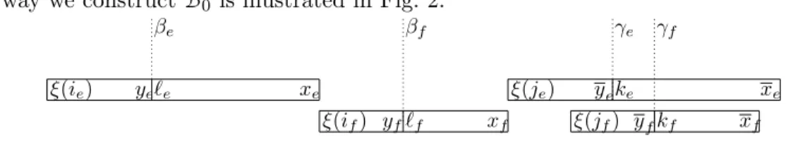
• the set of boundary relationsB0is obtained by putting the boundary relation (ξ(i), x, ξ(j), x) whenever (i, x, j, x) neither belongs toE nor is the dual of a boundary relation of E, and the boundary relations (ξ(ie), ye, ξ(je), ye), (`e, xe, ke, xe) and their duals for each e ∈E;
• the set (BH)0 contains ξΛ(BH) as well as the equation (ξ(ie) | `e) = (ξ(je) | ke), for each
e ∈E.
The way we construct B0 is illustrated in Fig. 2.
ξ(ie) xe ξ(je) xe
ξ(if) xf ξ(jf) xf
βe βf γe γf
ye`e yeke
yf`f yfkf
Figure 2: Factorization of (S, M), when E = {e, f}.
Proposition 32. The tripleM0 is a model ofS0 such that [S0,M0] = [S, M] and the Property (P.2)