On the Resilience of
Intrusion-Tolerant
Distributed Systems
Paulo Sousa
Nuno Ferreira Neves
Ant´
onia Lopes
Paulo Ver´ıssimo
DI–FCUL
TR–06–14
September 2006
Departamento de Inform´
atica
Faculdade de Ciˆ
encias da Universidade de Lisboa
Campo Grande, 1749–016 Lisboa
Portugal
Technical reports are available at http://www.di.fc.ul.pt/tech-reports. The files are stored in PDF, with the report number as filename. Alternatively, reports are available by post from the above address.
On the Resilience of Intrusion-Tolerant Distributed Systems
∗Paulo Sousa, Nuno Ferreira Neves, Ant´onia Lopes, Paulo Ver´ıssimo Departamento de Inform´atica
Faculdade de Ciˆencias da Universidade de Lisboa Campo Grande, 1749-016 Lisboa - Portugal
Abstract
The paper starts by introducing a new dimension along which distributed systems resilience may be evaluated – exhaustion-safety. A node-exhaustion-safe intrusion-tolerant distributed system is a sys-tem that assuredly does not suffer more than the assumed number of node failures (e.g., crash, Byzan-tine). We show that it is not possible to build this kind of systems under the asynchronous model. This result follows from the fact that in an asynchronous environment one cannot guarantee that the system terminates its execution before the occurrence of more than the assumed number of faults. After introducing exhaustion-safety, the paper proposes a new paradigm – proactive resilience – to build intrusion-tolerant distributed systems. Proactive resilience is based on architectural hybridiza-tion and hybrid distributed system modeling. The Proactive Resilience Model (PRM) is presented and shown to be a way of building node-exhaustion-safe intrusion-tolerant systems. Finally, the pa-per describes the design of a secret sharing system built according to the PRM. A proof-of-concept prototype of this system is shown to be highly resilient under different attack scenarios.
Key words: Intrusion tolerance, timing assumptions, proactive recovery, wormholes, secret
shar-ing
1
Introduction
A distributed system built under the asynchronous model makes no timing assumptions about the oper-ating environment: local processing and message deliveries may suffer arbitrary delays, and local clocks may present unbounded drift rates [17, 9]. In other words, in a (purely) asynchronous system it is not possible to guarantee that something will happen before a certain time. Therefore, if the goal is to build
∗This work was partially supported by the EC, through project IST-2004-27513 (CRUTIAL), and by the FCT, through the
dependable systems, the asynchronous model should only be used when system correctness does not depend on timing assumptions. At first sight, this conclusion only impacts the way algorithms are speci-fied, by disallowing their dependence on time (e.g., timeouts) in asynchronous environments. However, recently it was found that other types of timing dependencies exist in a more broader context orthogonal to algorithm specification [24]. In brief, every system depends on a set of resource assumptions (e.g., a minimum number of correct replicas), which must be met in order to guarantee correct behavior. If a resource degrades more than assumed during system execution, i.e., if the time until the violation of a resource assumption is bounded, then it is not safe to use the asynchronous model because one cannot ensure that the system will terminate before the assumption is violated.
Consider now that we want to build a dependable intrusion-tolerant distributed system, i.e., a dis-tributed system able to tolerate arbitrary faults, including malicious ones. In what conditions can one build such a system? Is it possible to build it under the asynchronous model?
This question was partially answered, twenty years ago, by Fischer, Lynch and Paterson [10], who proved that there is no deterministic protocol that solves the consensus problem is an asynchronous distributed system prone to even a single crash failure. This impossibility result (commonly known as FLP) has been extremely important, given that consensus lies at the heart of many practical problems, including membership, atomic commitment, leader election, and atomic broadcast. Considerable amount of research addressed solutions to this problem, trying to preserve the desirable independence from timing assumptions at algorithmic level. One could say that the question asked above was well on its way of being answered. However, as mentioned before, a new and surprising dependence on timing was found recently [24]. The present paper builds on this previous result.
In the first part of the paper, we show that assuming a maximum number of f faulty nodes under the asynchronous model is dangerous. Given that an asynchronous system may have a potentially long execution time, there is no way of assuring that no more than f faults will occur, specially in malicious en-vironments. This intuition is formalized through the introduction of exhaustion-safety – a new dimension over which distributed systems resilience may be evaluated. A node-exhaustion-safe intrusion-tolerant distributed system is a system that assuredly does not suffer more than the assumed number of node failures: depending on the system, nodes may fail by crash, or start behaving in a Byzantine way, or dis-close some secret information, and all these types of failures may be caused by accidents (e.g., a system bug), or may be provoked by malicious actions (e.g., an intrusion perpetrated by a hacker). We show that it is not possible to build any type of node-exhaustion-safe distributed f intrusion-tolerant system under the asynchronous model. In fact, we achieve a more general result, and show that it is impossible,
under the asynchronous model, to avoid the exhaustion of any resource with bounded exhaustion time. Despite this general result, the focus on this paper is on fault/intrusion-tolerant distributed systems and on node-exhaustion-safety.
Our result is orthogonal to FLP. Whereas FLP shows that a class of problems has no deterministic solution in asynchronous systems subjected to failures, our result applies to all types of asynchronous distributed systems, independently of the specific goal/protocols of the system.
What are then the minimum synchrony requirements in order to build a dependable intrusion-tolerant distributed system?
If the system needs consensus (or equivalent primitives), then Chandra and Toueg [7] showed that consensus can be solved in asynchronous systems augmented with failure detectors (FDs). The main idea is that FDs operate under a more synchronous environment and can therefore offer a service (the failure detection service) with sufficient properties to allow consensus to be solved.
But what can one say about intrusion-tolerant asynchronous systems that do not need consensus? Obviously, they are not affected by the FLP result, but are they dependable?
Notice that, with regard to exhaustion-safety, an asynchronous consensus-free system is the same as an asynchronous consensus-based system enhanced with synchronous failure detectors. So, the question remains: What are the minimum synchrony requirements to build a dependable (exhaustion-safe) intrusion-tolerant distributed system? In this paper such minimum requirements are not pursued, but instead we describe a set of (sufficient) conditions that enable the construction of certain types of exhaustion-safe systems.
To achieve exhaustion-safety, the goal is to guarantee that the assumed number of faults is never exceeded. In this context, proactive recovery seems to be a very interesting approach [19]. The aim of proactive recovery is conceptually simple – components are periodically rejuvenated to remove the effects of malicious attacks/faults. If the rejuvenation is performed frequently often, then an adversary is unable to corrupt enough resources to break the system. Therefore, proactive recovery has the potential to support the construction of resilient intrusion-tolerant distributed systems. However, in order to achieve this, proactive recovery needs to be architected under a sufficiently strong model that allows regular rejuvenation of the system. In fact, proactive recovery protocols (like FDs) typically require stronger environment assumptions (e.g., synchrony, security) than the rest of the system (i.e., the part that is proactively recovered).
In the second part of the paper, we propose proactive resilience – a new and more resilient approach to proactive recovery based on hybrid distributed system modeling [26] and architectural
hybridiza-tion [25]. It is argued that the architecture of a system enhanced with proactive recovery should be hybrid, i.e., divided in two parts: the “normal” payload system and the proactive recovery subsystem, the former being proactively recovered by the latter. Each of these two parts should be built under differ-ent timing and fault assumptions: the payload system may be asynchronous and vulnerable to arbitrary faults, and the proactive recovery subsystem should be constructed in order to assure a more synchronous and secure behavior.
We describe a generic Proactive Resilience Model (PRM), which proposes to model the proactive recovery subsystem as an abstract component – the Proactive Recovery Wormhole (PRW). The PRW may have many instantiations depending on the application/protocol proactive recovery needs (e.g., re-juvenation of cryptographic keys, restoration of system code). Then, it is shown that the PRM can be used to build node-exhaustion-safe intrusion-tolerant distributed systems.
Finally, the paper describes the design of a distributed f intrusion-tolerant secret sharing system, which makes use of a specific instantiation of the PRW targeting the secret sharing scenario [22]. This system is shown to be node-exhaustion-safe under certain conditions mainly related to the adversary power, and we built a proof-of-concept prototype in which it is showed that exhaustion-safety is ensured even in the presence of fierce adversaries.
2
Exhaustion-Safety
Typically, the correctness of a protocol depends on a set of assumptions regarding aspects like the type and number of faults that can happen, the synchrony of the execution, etc. These assumptions are in fact an abstraction of the actual resources the protocol needs to work correctly (e.g., when a protocol assumes that messages are delivered within a known bound, it is in fact assuming that the network will have certain characteristics such as bandwidth and latency). The violation of these resource assumptions may affect the safety and/or liveness of the protocol. If the protocol is vital for the operation of some system, then the system liveness and/or safety may also be affected.
To formally define and reason about exhaustion-safety of systems with regard to a given resource assumption, it is necessary to adopt a suitable model. Let ϕr be a resource assumption on a resource
r. We consider models which define (i) for every system S, the set of its executionsJSK = {E : E is a S−execution}, which is a subset of the set EX EC that contains all possible executions of any system
(i.e.,JSK ⊆ E X EC), and (ii) a set |= ϕr, s.t. |= ϕr⊆ EXEC is the subset of all possible executions that
the executionE .
In the context of such models, exhaustion-safety is defined straightforwardly.
Definition 2.1. A system S is r-exhaustion-safe wrt ϕrif and only if ∀E ∈JSK : E |= ϕr.
Notice that this formulation allows one to study the exhaustion-safety of a system for different types of assumptions ϕron a given resource r.
2.1 The Resource Exhaustion Model
Our main goal is to formally reason about how exhaustion-safety may be affected by different combi-nations of timing and fault assumptions. So, we need to conceive a model in which the impact of those assumptions can be analyzed. We call this model the Resource EXhaustion model (REX ).
Our model considers systems that have a certain mission. Thus, the execution of this type of sys-tems is composed of various processing steps needed for fulfilling the system mission (e.g., protocol executions). We define two intervals regarding the system execution and the time necessary to exhaust a resource, defined by: execution time and exhaustion time. The exhaustion time concerns a specific resource assumption ϕr on a specific resource r. Therefore, in what follows, JSK denotes the set of
executions of a system S under REX for a fixed assumption ϕron a specific resource r.
Definition 2.2. A system executionE is a pair hTexec, Texhi, where
• Texec∈ℜ+0 and represents the total execution time;
• Texh∈ℜ+0 and represents the time necessary, since the beginning of the execution, for assumption
ϕrto be violated.
The proposed notion of system execution captures the execution time of the system and the time necessary for assumption ϕr to be violated in a specific run. Notice that, in this way, one captures the
fact that the time needed to violate a resource assumption may vary from execution to execution. For instance, if a system suffers upgrades between executions, its exhaustion time may be, consequently, increased or decreased.
Definition 2.3. The assumption ϕr is not violated during a system execution E , which we denote by
E |= ϕr, if and only if TexecE < TexhE .
By combining Definitions 2.1 and 2.3, we can derive the definition of an r-exhaustion-safe system under REX .
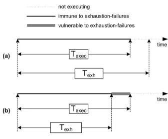
time Texec Texh not executing immune to exhaustion-failures vulnerable to exhaustion-failures (a) time Texec Texh (b)
Figure 1: (a) An execution not violating ϕr; (b) An execution violating ϕr.
Proposition 2.4. A system S is r-exhaustion-safe wrt a given assumption ϕr if and only if ∀E ∈JSK :
TexecE < TexhE .
This corollary states that a system is r-exhaustion-safe if and only if resource exhaustion (i.e., the violation of ϕr) does not occur during any execution. Notice that, even if the system is not
exhaustion-safe, it does not mean that the system fails immediately after resource exhaustion. In fact, a system may even present a correct behavior between the exhaustion and the termination events. Thus, a non
exhaustion-safe system may execute correctly during its entire lifetime. However, after resource
exhaustion there is no guarantee that an exhaustion-failure will not happen. Figure 1 illustrates the differences between an execution of a (potentially) exhaustion-safe system and a “bad” execution of a non safe system. An safe system is always assuredly immune to exhaustion-failures. A non exhaustion-safe system has at least one execution (such as the one depicted in Figure 1b) with a period of vulnerability to exhaustion-failures (the shaded part of the timeline) where the resource is exhausted and thus correctness may be compromised.
In a distributed fault-tolerant system, nodes are important resources, so important that one typically makes the assumption that a maximum number f of nodes can fail during its execution, and the system is designed in order to resist up to f node failures. This type of systems can be analyzed under the REX model, nodes being the resource considered, and the assumption ϕnodebeing equal to nf ail≤ f , where
nf ail represents the maximum number of nodes which, during an execution, are failed at any time. In
other words, this assumption means that no more than f nodes can be failed simultaneously. Notice that in a system in which failed nodes do not recover, this assumption is equivalent to assuming that no more
than f node failures can occur during the system execution.
According to Proposition 2.4, a system whose failed nodes do not recover is node-exhaustion-safe if and only if every execution terminates before the time needed for f + 1 node failures to be produced. In order to build a node-exhaustion-safe fault-tolerant system, one would like to forecast the maximum number of failures bound to occur during any execution, call it Nf ail, so that the system is designed to
handle f = Nf ail failures.
As Section 3 will show, the key aspect of the study of this model is that condition TexecE < TexhE can be evaluated, that is, that we can determine whether it is maintained, or not, depending on the type of system assumptions. Note that the idea is not to know the exact values of TexecE and TexhE , but rather to reason about constraints that may be imposed on them, derived from environment and/or algorithmic assumptions. So, when we analyze a given system S under the REX model, we may happen to know a set of hTexecE , TexhE i values for some already finished executions, and evaluate these known values, which may
indicate that the system is non exhaustion-safe. However, much more important than that would be to predict, at system or even at algorithm design time, if the system is (always) exhaustion-safe according to the environment assumptions. This would allow us, as we shall show, to make propositions about exhaustion-safety for categories of algorithms and system fault and synchrony models. With this goal in mind, we start by defining two crucial properties of the model, which follow immediately from the previous definitions.
Property 2.5. A sufficient condition for S to be r-exhaustion-safe wrt ϕris
∃Texecmax∈ℜ
+
0(∀E ∈JSK : TexecE ≤ Texecmax) ∧ (∀E ∈JSK : TexhE > Texecmax)
Property 2.6. A necessary condition for S to be r-exhaustion-safe wrt ϕris
∃Texhmax∈ℜ
+
0(∀E ∈JSK : TexhE ≤ Texhmax) ⇒ (∀E ∈JSK : TexecE < Texhmax)
Property 2.5 states that a system S is r-exhaustion-safe wrt ϕrif there exists an upper-bound Texecmax
on the system execution time, and if the exhaustion time of every execution is greater than Texecmax.
Property 2.6 states that a system S can only be r-exhaustion-safe wrt ϕr if, given an upper-bound
Texhmax on the system exhaustion time, the execution time of every execution is lower than Texhmax.
3
Exhaustion-Safety vs Synchrony Assumptions
3.1 Synchronous Systems
Systems developed under the synchronous model are relatively straightforward to reason about and to describe. This model has three distinguishing properties that help us understand better the system be-havior: there is a known time bound for the local processing of any operation, message deliveries are performed within a well-known maximum delay, and components have access to local clocks with a known bounded drift rate with respect to real time [14, 27].
If one considers a synchronous system S with a bounded lifetime under REX , then it is possible to use the worst-case bounds defined during the design phase to assess the conditions of r-exhaustion-safety, for given r and ϕr.
Corollary 3.1. If S is a synchronous system with a bounded lifetime Texecmax (i.e., ∀E ∈JSK : TexecE ≤
Texecmax) and ∀E ∈JSK : TexhE > Texecmax, then S is r-exhaustion-safe wrt ϕr.
Proof. See Property 2.5.
Therefore, if one wants to design an exhaustion-safe synchronous system with a bounded lifetime, then one has to guarantee that no exhaustion is possible during the limited period of time delimited by
Texecmax. For instance, and getting back to our previous example, in a distributed f fault-tolerant system
this would mean that no more than f node failures should occur within Texecmax.
Note that Corollary 3.1 only applies to synchronous systems with a bounded lifetime. A synchro-nous system may however have an unbounded lifetime. This seems contradictory at first sight and thus deserves a more detailed explanation. A synchronous system is typically composed by a set of (synchro-nous) rounds with bounded execution time (e.g., a synchronous server replying to requests from clients, each pair request-reply being a round). However, the number of rounds is not necessarily bounded. We consider that a synchronous system has a bounded lifetime if the number of rounds is bounded. Other-wise, the system has unbounded lifetime. If the system lifespan is unbounded, and Texh is bounded, then
we can prove the following.
Corollary 3.2. If S is a synchronous system with an unbounded lifetime (i.e., @Texecmax∈ℜ
+
0, ∀E ∈JSK :
TexecE ≤ Texecmax) and ∃Texhmax ∈ℜ
+
0, ∀E ∈JSK : TexhE ≤ Texhmax, then S is not r-exhaustion-safe wrt ϕr.
Proof. If the set {TexecE :E ∈JSK} does not have a bound, it is impossible to guarantee that TexecE < Texhmax,
for everyE ∈JSK and, therefore, by Property 2.6, S is not r-exhaustion-safe.
In fact, synchronous systems may suffer accidental or malicious faults. These faults may have two bad effects: provoking timing failures that increase the expected execution time; causing resource
degradation, e.g., node failures, which decrease Texh. Notice that both these effects force the conditions
of Corollary 3.2. Thus, in a synchronous system, an adversary can not only perform attacks to exhaust resources, but also violate the timing assumptions, even if during a limited interval. For this reason, there is currently among the research community a common belief that synchronous systems are fragile, and that secure systems should be built under the asynchronous model.
3.2 Asynchronous Systems
The distinguishing feature of an asynchronous system is the absence of timing assumptions, which means arbitrary delays for the execution of operations and message deliveries, and unbounded drift rates for the local clocks [10, 17, 9]. This model is quite attractive because it leads to the design of programs and components that are easier to port or include in different environments.
If one considers a distributed asynchronous system S under REX , then S can be built in such a way that termination is eventually guaranteed (sometimes only if certain conditions become true). However, it is impossible to determine exactly when termination will occur. In other words, the execution time is unbounded. Therefore, all we are left with is the relation between Texecand Texh, in order to assess if S is
r-exhaustion-safe, for given r and ϕr.
Can a distributed asynchronous system S be r-exhaustion-safe? Despite the arbitrariness of Texec,
the condition TexecE < TexhE must always be maintained. Given that TexecE may have an arbitrary value, impossible to know through aprioristic calculations, the system should be constructed in order to ensure that, in all executions, TexhE is greater than TexecE . This is very hard to achieve for some types of r and
ϕr. An example is assuring that no more than f nodes ever fail. We provide a solution to this particular
case in the next section based on a hybrid system architecture that guarantees exhaustion-safety through a synchronous subsystem that executes periodic rejuvenations.
If one assumes that the system is homogeneously asynchronous, and that the set {TexhE :E ∈JSK} is
bounded, one can prove the following corollary of Property 2.6, similar to Corollary 3.2:
Corollary 3.3. If S is an asynchronous system (and, hence, @Texecmax∈ℜ
+
0, ∀E ∈JSK : TexecE ≤ Texecmax)
and ∃Texhmax∈ℜ
+
0, ∀E ∈JSK : TexhE ≤ Texhmax, then S is not r-exhaustion-safe wrt ϕr.
Proof. See Corollary 3.2.
This corollary is generic, in the sense that it applies to any type of system with a bounded Texh for
some assumption ϕr. However, its implications on distributed f fault-tolerant systems deserve a special
Even though real distributed systems working under the asynchronous model have a bounded Texh
in terms of node failures, they have been used with success for many years. This happens because, until recently, only accidental faults (e.g., crash or omission) were a threat to systems. This type of faults, being accidental by nature, occur in a random manner. Therefore, by studying the environment in detail and by appropriately conceiving the system (e.g., estimate an upper bound on Texecthat applies to a large
number of executions), one can achieve an asynchronous system that behaves as if it were exhaustion-safe, with a high probability. That is, despite having the failure syndrome as it was proved, it would be very difficult to observe it in practice.
However, when one starts to consider malicious faults, a different reasoning must be made. This type of faults is intentional (not accidental) and therefore their distribution is not random: the actual distribution may be shaped at will by an adversary whose main purpose is to break the system (e.g., force the system to execute during more time than any estimated upper bound on Texec). In these conditions,
having a bounded Texh(e.g., stationary maximum bound for node failures) may turn out to be catastrophic
for the safety of the system. That is, the comments above regarding accidental faults do not apply to intrusion-tolerant systems working under the asynchronous model.
Consequently, Texh should not have a bounded value in an asynchronous distributed fault-tolerant
system operating in a environment prone to anything more severe than accidental faults. The goal should then be to maintain Texhabove Texec, in all executions.
4
An Architectural Hybrid Model for Proactive Recovery
4.1 Proactive Recovery
One of the most interesting approaches to avoid resource exhaustion due to accidental or malicious cor-ruption of components is through proactive recovery [19], which can be seen as a form of dynamic redundancy [23]. The aim of this mechanism is conceptually simple – components are periodically re-juvenated to remove the effects of malicious attacks/faults. If the rejuvenation is performed frequently often, then an adversary is unable to corrupt enough resources to break the system. Proactive recovery has been suggested in several contexts. For instance, it can be used to refresh cryptographic keys in order to prevent the disclosure of too many secrets [16, 15, 12, 30, 4, 29, 18]. It may also be utilized to restore the system code from a secure source to eliminate potential transformations carried out by an adversary [19, 6]. Moreover, it may encompass the substitution of software components to remove vulnerabilities existent in previous versions (e.g., software bugs that could crash the system or errors
exploitable by outside attackers). Vulnerability removal can also be done through address space random-ization [3, 2, 11, 20, 28], which could be used to periodically randomize the memory location of all code and data objects.
Thus, intuitively, by using a well-planned strategy of proactive recovery, Texh can be recurrently
increased in order that it is always greater than Texecin all executions. However, this intuition is rather
difficult to substantiate if the system is asynchronous. The simple task of timely triggering a periodic recovery procedure is impossible to attain under the pure asynchronous model, namely if it is subject to malicious faults. From this reasoning, and according to Corollary 3.3, one can conclude that it is not possible to ensure the exhaustion-safety of an asynchronous system with bounded exhaustion time through asynchronous proactive recovery. For a detailed discussion on this topic, see [24].
The impossibility of building an exhaustion-safe f fault/intrusion-tolerant distributed asynchronous system, namely in the presence of malicious faults, and even if enhanced with asynchronous proactive recovery, lead us to investigate hybrid models for proactive recovery.
4.2 The Proactive Resilience Model
Proactive recovery is useful to periodically rejuvenate components and remove the effects of malicious attacks/failures, as long as it has timeliness guarantees. In fact, the rest of the system may even be completely asynchronous – only the proactive recovery mechanism needs synchronous execution. This type of requirement made us believe that one of the possible approaches to use proactive recovery in an effective way, is to model and architect it under a hybrid distributed system model [26].
In this context, we propose the Proactive Resilience Model (PRM) – a more resilient approach to proactive recovery based on the Wormholes distributed system model [26]. The PRM defines a system enhanced with proactive recovery through a model composed of two parts: the proactive recovery sub-system and the payload sub-system, the latter being proactively recovered by the former. Each of these two parts obeys different timing assumptions and different fault models, and should be designed accordingly. The payload system executes the “normal” applications and protocols. Thus, the payload synchrony and fault model entirely depend on the applications/protocols executing in this part of the system. For instance, the payload may operate in an asynchronous Byzantine environment.
The proactive recovery subsystem executes the proactive recovery protocols that rejuvenate the ap-plications/protocols running in the payload part. This subsystem is more demanding in terms of timing and fault assumptions, and it is modeled as an abstract distributed component called Proactive Recovery
local PRW CY1 control network Host D Host E local PRW CY2 payload network local PRW CX1 control network
Host A Host B Host C
cluster CX with three interconnected local PRWs
local PRW CX2 local PRW CX3 payload network local PRW CZ1 Host F payload network synchronous & secure
any synchrony & security (payload)
cluster CY with two interconnected local PRWs
cluster CZ with a single local PRW
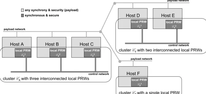
Figure 2: The architecture of a system with a PRW.
specific instantiation is chosen according to the concrete application/protocol that needs to be proactively recovered.
The architecture of a system with a PRW is suggested in Figure 2; there is a local module in every host, called the local PRW. These modules are organized in clusters, called PRW clusters, and the local PRWs in each cluster are interconnected by a synchronous and secure control network. The set of all PRW clusters is what is collectively called the PRW. The PRW is used to execute proactive recovery procedures of protocols/applications running between participants in the hosts concerned, on any usual distributed system architecture (e.g., the Internet).
Conceptually, a local PRW is a module inside a host and separated from the OS. In practice, this conceptual separation between the local PRW and the OS can be achieved in either of two ways: (1) the local PRW can be implemented in a separate, tamper-proof hardware module (e.g., PC appliance board) and so the separation is physical; (2) the local PRW can be implemented on the native hardware, with a virtual separation and shielding between the local PRW and the OS processes implemented in software.
The way clusters are organized is dependent on the rejuvenation requirements. Typically, a clus-ter is composed of nodes that are somehow inclus-terdependent w.r.t. rejuvenating (e.g., need to exchange information during recovery). In this paper we focus on two specific cluster configurations:
PRWl is composed of n clusters, each one including a single local PRW. Therefore, every PRWl cluster is exactly like clusterCZdepicted in Figure 2, and, consequently, no control network exists in any
PRWd is composed of a single cluster including all local PRWs. For instance, if the system was composed of 3 nodes, then the (single) PRWd cluster would be like clusterCX depicted in Figure 2. In this
case every local PRW is interconnected through the same control network.
PRWl should be used in scenarios where the recovery procedure only requires local information,
and therefore there is no need for distributed execution (e.g., rebooting a stateless replicated system from clean media in order to remove malware programs). PRWd should be used when the recovery is done through a fully distributed recovery procedure in which every local PRW should participate (e.g., proactive secret sharing as explained in Section 5). Many more configurations are possible, namely configurations composed of heterogeneous clusters (i.e., clusters with different sizes). We leave the discussion of such configurations and their usefulness as future work.
4.2.1 Periodic Timely Rejuvenation
The PRW executes periodic rejuvenations through a periodic timely execution service. This section defines the periodic timely execution service, proposes an algorithm to implement it, and specifies the real-time guarantees required of the PRW. Then, assuming that the local PRWs do not fail, Section 4.2.2 proves that systems enhanced with a PRW executing an appropriate periodic timely rejuvenation service are assuredly node-exhaustion-safe. Section 4.2.2 also discusses how this result can be generalized in order to take into account potential crashes of local PRWs.
Each PRW cluster runs its own instance of the periodic timely execution service, and there are no constraints in terms of the coordination of the different instances. Albeit running independently, each cluster offers the same set of properties dictated by four global parameters: F, TP, TDand Tπ. Namely,
each cluster executes a rejuvenation procedure F in rounds, and each round is triggered within TP from
the last triggering. This triggering is done by at least one local PRW (in each cluster), and every other local PRWs (of the same cluster) start executing the same round within Tπof each other. Moreover, each
cluster guarantees that, once all local PRWs are in the same round, the execution time of F is bounded by
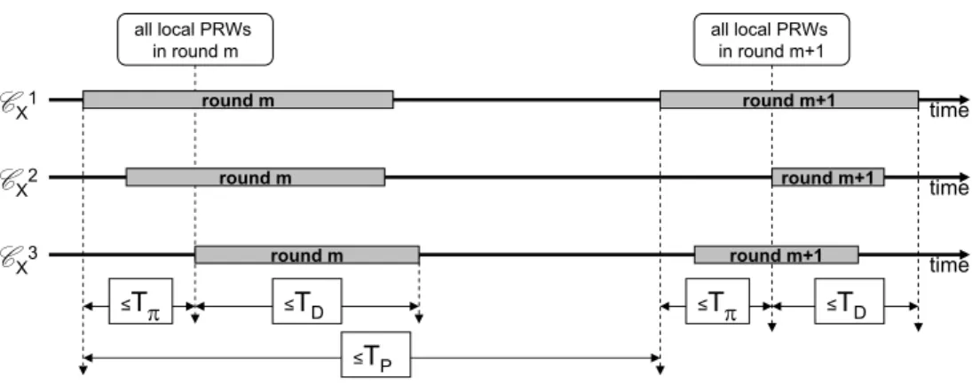
TD. Therefore, the worst case execution time of each round of F is given by Tπ+ TD. Figure 3 illustrates
the relationship between TP, TD, and Tπ, in a cluster with three local PRWs. A formal definition of the
periodic timely execution service is presented next. The definition is generic, in the sense that it applies to generic components and not only local PRWs.
Definition 4.1. Let F be a procedure and TD, TP, Tπ ∈ℜ +
0, s.t. TD+ Tπ < TP. A set of components
time time time ≤TP ≤Tπ ≤TD ≤Tπ ≤TD round m round m round m+1 round m+1 round m+1 all local PRWs in round m all local PRWs in round m+1 round m
C
X1C
X2C
X3Figure 3: Relationship between TP,TDand Tπin a clusterCX with three local PRWs.
hF, TD, TP, Tπi, if and only if:
1. the components of the same clusterCiexecute F in rounds, and therefore F is a distributed
proce-dure within a cluster;
2. for every real time instant t ofC execution time, there exists a round of F triggered in each cluster
Ciwithin TP from t, i.e., one component C in each clusterCitriggers the execution of a round of
F within TPfrom t;
3. every component in a clusterCi triggers the execution of the same round of F within Tπ of each
other component in the same cluster;
4. each clusterCiensures that, once all components are in the same round of F, the execution time
of F is bounded by TD, i.e., the difference between the real time instant when the last component
in a clusterCi starts executing F and the real time instant when the last component of the same
cluster finishes executing is not greater than TD(both executions refer to the same round).
Corollary 4.2. If C is a set of components, organized in s clusters C1, ...,Cs, that offers a periodic
timely execution service hF, TD, TP, Tπi then, for every real time instant t ofC execution time, there exists
a round of F triggered in each clusterCiwithin TPfrom t that is terminated within TP+ TD+ Tπfrom t.
Definition 4.3. A system enhanced with a PRW (hF, TD, TP, Tπi) has a local PRW in every host.
More-over these are organized in clusters and in conjunction offer the periodic timely execution service
hF, TD, TP, Tπi.
As mentioned before, the PRW admits two particular cluster configurations — PRWl and PRWd. These are defined as follows.
Definition 4.4. A system enhanced with a PRWl(hF, TD, TP, Tπi) is a system enhanced with a
PRW (hF, TD, TP, Tπi) s.t. there exists n clustersC1, ...,Cn, and each clusterCi is composed of a single
local PRW.
Definition 4.5. A system enhanced with a PRWd(hF, TD, TP, Tπi) is a system enhanced with a
PRW (hF, TD, TP, Tπi) s.t. there exists a single clusterC1comprising all local PRWs.
A periodic timely execution service can be built using, for instance, Algorithm 1, and a construction process that ensures the following properties:
P1 There exists a known upper bound on the processing delays of every local PRW. P2 There exists a known upper bound on the clock drift rate of every local PRW.
P3 There exists a known upper bound on the message delivery delays of every control network inter-connecting the local PRWs of a same cluster.
Suppose that each local PRW executes Algorithm 1, where function clock returns the current value of the clock of the local PRW, F is the recovery procedure that should be periodically timely executed, and TP is the desired recovery periodicity. Value δ defines a safety time interval used to guarantee that
consecutive recoveries are triggered within TP from each other in the presence of the assumed upper
bounds on the processing delays (P1) and the clock drift rate (P2). Notice that between the wait instruc-tion in line 2 and the triggering of F in line 7, there is a set of instrucinstruc-tions that take (bounded) time to execute. δ should guarantee that consecutive recoveries are always triggered within TP of each other
independently of the actual execution time of those instructions, and taking into account the maximum possible clock drift rate. However, δ should also guarantee that every local PRW triggers F within Tπ
of each other. So, δ should not be greater than TP− (TD+ Tπ) in order to ensure that the local PRW
Ci1 in each clusterCi does not start to execute F too early (i.e., when other local PRWs may still be
executing the previous round). In these conditions, the algorithm guarantees that F is always triggered, in each cluster Ci, by local PRWsCi1 within TP from the last triggering. Moreover, given that it is
assured that different rounds do not overlap, the triggering instant in the local PRWs of the same cluster differs in at most the maximum message delivery delay (P3) plus the maximum processing delay, i.e., the time necessary for message trigger to be delivered and processed in all local PRWs. Thus, the value of Tπ is defined by this sum. In this situation, each local PRW offers a periodic timely execution
ser-vice PRW (hF, TD, TP, Tπi) provided they ensure that, once all local PRWs are in the same round of F, its
Algorithm 1: Periodic timely execution service run by each local PRWCij in clusterCi
initialization: tlast← clock
begin
while true do
// local PRWsCijwith j = 1 in each clusterCicoordinate the recovering process
if j = 1 then
1
wait until clock = tlast+ TP− δ 2 tlast← clock 3 multicast(trigger,Ci) 4 else 5 receive(trigger) 6 execute F 7 end
4.2.2 Building Node-Exhaustion-Safe Systems
A system enhanced with a PRW (hF, TD, TP, Tπi) can be made node-exhaustion-safe under certain
condi-tions, as it will be shown in Theorem 4.6. This theorem states that if it is possible to lower-bound the exhaustion time (i.e., the time needed to produce f + 1 node failures) of every system execution by a known constant Texhmin, then node-exhaustion-safety is achieved by assuring that TP+ TD+ Tπ< Texhmin.
In what follows, let JSK denote the set of executions of an f fault-tolerant distributed system S
under the REX model for the condition ϕnode= nf ail≤ f , where nf ail represents the maximum number
of nodes which, during an execution, are failed simultaneously. Notice that the type of failure is not specified, but only that nodes may fail in some way and that this failure can be recovered through the execution of a rejuvenation procedure. A node failure may be for instance the disclosure of some secret information (the type of failures considered in Section 5), or a hacker intrusion that compromises the behavior of some parts of the system. Notice also that the rejuvenation procedure will depend on the type of failure considered. For instance, whereas a hacker intrusion may require the reboot of the system and the reloading of code and state from some trusted source, the disclosure of secret information may be solved by simply turning that information obsolete.
Theorem 4.6. Suppose that
inf({TexhE :E ∈JSK})1;
2. the time needed to produce f + 1 (≤ n) node failures at any instant is independent of the number of nodes that are currently failed;
3. F is a distributed procedure that upon termination ensures that all nodes involved in its execution are not failed.
Then, the system S, enhanced with a PRW (hF, TD, TP, Tπi) s.t. TP+ TD+ Tπ< Texhmin is
node-exhaustion-safe w.r.t. ϕnode.
Proof. Assumption (1) entails that, in every execution of S, from a state with 0 failed nodes, it takes at
least Texhmin for f + 1 node failures to be produced. Let m be a natural number such that m + f + 1 ≤ n.
Then, using assumption (2), we may conclude that, in every execution of S, it takes at least Texhmin to
reach a state with m + f + 1 failed nodes from a state with m failed nodes2. This also means that :
4. in every execution of S, the number of node failures during a time interval ]t,t + Texhmin[ is at most
f .
By contradiction, assume that there exists an execution of the system S, enhanced with a
PRW (hF, TD, TP, Tπi) s.t. TP+ TD+ Tπ< Texhmin, that violates ϕr. This means that there is a time instant
tC when there are more than f failed nodes. Notice that tC cannot occur in less than Texhmin from the
system initial start instant, because this would mean that more than f + 1 node failures were produced in less than Texhmin from a state with 0 failed nodes, which is contradictory with assumption (1). Hence,
tCoccurs in at least Texhmin from the system initial start instant. Then, by (4), because in less than Texhmin
is not possible that more than f nodes become failed, in tI= tC− Texhmin there is at least one failed node.
Given that we assumed that the PRW never fails and given that the nature of F is to recover the nodes of the cluster where F is executed (assumption (3)), the execution of S under PRW (hF, TD, TP, Tπi) with
TP+ TD+ Tπ< Texhmin ensures that any node that is failed at tIis recovered no later than tI+ TP+ TD+ Tπ
and, hence, is recovered earlier than tC= tI+ Texhmin. If one of the nodes that are failed in tI becomes
recovered before tC and there are more than f failed nodes in tC= tI+ Texhmin, then more than f nodes
become failed in the interval ]tI,tI+ Texhmin[. But this is contradictory with (4) above.
1inf() denotes the infimum of a set of real numbers, i.e., the greatest lower bound for the set.
2Notice that a node may fail, be recovered, fail again, and so on. Therefore, the total number of node failures does not correspond necessarily to the number of currently failed nodes.
From Theorem 4.6 it follows that, in order to build a node-exhaustion-safe intrusion-tolerant system, the system architect should choose an appropriate degree of fault-tolerance f , such that TP+ TD+ Tπ <
TexhE , for every system executionE . In other words, any interval with length TP+ TD+ Tπshould not be
sufficient for f + 1 node failures to be produced, throughout the lifetime of the system.
As mentioned before, the results presented in this section depend on the assumption that local PRWs never fail. This assumption allows to abstract from PRWs crashes and, in this way, allows to focus on what it is really important. However, Theorem 4.6 could be extended to the case where the number of crashes is upper-bounded by some known constant fc. The difference would be that one would need
to add sufficient redundancy to the system in order to resist the fc possible crashes, and the protocol(s)
executed by the PRW would also have to take this into account. Section 5 explains how this could be done in a concrete scenario. In order to minimize the probability of crashing more than fc local
PRWs, and in this way guarantee the exhaustion-safety of the overall system, the system architect would need to estimate the probability of crash according to environment conditions and/or apply techniques of dynamic redundancy, where crashed PRWs could be repaired or replaced before more than fcbecome
crashed.
In the next section, the Proactive Resilience Model is applied to a concrete algorithmic scenario as a proof of concept. We present a proactive secret sharing wormhole, showing how the resilience of a secret sharing protocol can be enhanced using our model.
5
The Proactive Secret Sharing Wormhole
Secret sharing schemes protect the secrecy and integrity of secrets by distributing them over different locations. A secret sharing scheme transforms a secret s into n shares s1, s2, ..., snwhich are distributed
to n share-holders. In this way, the adversary has to attack multiple share-holders in order to learn or to destroy the secret. For instance, in a (k + 1, n)-threshold scheme, an adversary needs to compromise more than k share-holders to learn the secret, and corrupt at least n − k shares in order to destroy the same secret.
Various secret sharing schemes have been developed to satisfy different requirements. This paper uses the Shamir’s approach [22] to implement a (k + 1, n)-threshold scheme. This scheme can be defined as follows: given an integer-valued secret s, pick a prime q which is bigger than both s and n. Randomly choose a1, a2, ..., ak from [0, q[ and set polynomial f (x) = (s + a1x + a2x2+ ... + akxk) mod q. For i =
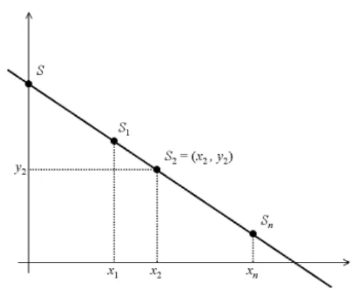
Figure 4: Shamir’s secret sharing scheme for k = 1.
providing their shares and using polynomial interpolation to compute s. Moreover, given k or fewer shares, it is impossible to reconstruct s.
A special case where k = 1 (that is, two shares are required for reconstructing the secret), is given in Figure 4. The polynomial is a line and the secret is the point where the line intersects with the y-axis (i.e., (0, f (0)) = (0, s)). Each share is a point on the line. Any two (i.e., k + 1) points determine the line and hence the secret. With just a single point, the line can be any line that passes the point, and hence its insufficient to determine the right y-axis cross point.
In many applications, a secret s may be required to be held in a secret-sharing manner by n share-holders for a long time. If at most k share-share-holders are corrupted throughout the entire lifetime of the secret, any (k + 1, n)-threshold scheme can be used. In certain environments, however, gradual break-ins into a subset of locations over a long period of time may be feasible for the adversary. If more than k share-holders are corrupted, s may be stolen. An obvious defense is to periodically refresh s, but this is not possible when s corresponds to inherently long-lived information (e.g., cryptographic root keys, legal documents).
In consequence, what is actually required to protect the secrecy of the information is to be able to periodically renew the shares without changing the secret. Proactive secret sharing (PSS) was introduced in [16] in this context. In PSS, the lifetime of a secret is divided into multiple periods and shares are renewed periodically. In this way, corrupted shares will not accumulate over the entire lifetime of the secret since they are checked and corrected at the end of the period during which they have occurred. A (k + 1, n) proactive threshold scheme guarantees that the secret is not disclosed and can be recovered as long as at most k share-holders are corrupted during each period, while every share-holder may be corrupted multiple times over several periods.
the calculation of s. The goal of proactive secret sharing is to harden the difficulty of an adversary being able to collect a set of k + 1 consistent shares. This is done by periodically changing the shares, assuring that the interval between consecutive share rejuvenations is not sufficient for an adversary to collect k + 1 (consistent) shares.
In this section, we address the exhaustion-safety of distributed systems based on secret sharing, i.e., the assumption ϕnodeis nf ail≤ k, where nf ailrepresents the maximum number of consistent shares that,
during an execution, are disclosed simultaneously. A share is considered disclosed when it is known by an adversary.
We propose the Proactive Secret Sharing Wormhole (PSSW) as an instantiation of the
PRWdhF, TD, TP, Tπi presented in Section 4.2. Notice that this means that there exists a single cluster
composed of all local PSSWs and therefore all local PSSWs are interconnected by the same synchronous and secure control network. The PSSW targets distributed systems which are based on secret sharing and the goal of the PSSW is to periodically rejuvenate the secret share of each node, so that the overall system is exhaustion-safe wrt ϕnode.
The presentation of the PSSW is divided in two parts. The first part describes the procedure re-fresh sharethat renews the shares without changing or disclosing the secret, and enumerates the assump-tions that need to be ensured in the construction of the PSSW. The second part discusses how the values of TP, TDand Tπ may be chosen in order to ensure that a secret sharing system enhanced with a PSSW
= PRWdhrefresh share , TD, TP, Tπi is exhaustion-safe wrt ϕnode. The choice of the values TD, TP, Tπ is
conditioned by the PSSW assumptions, including the assumed adversary power.
The PSSW executes Algorithm 1 in order to periodically and timely execute the procedure re-fresh share presented in Algorithm 2. This procedure is based on the share renewal scheme of [16]. In lines 1–2, local PSSW i picks k random numbers {δim}m∈{1...k} in [0, q[. These numbers define the
polynomial δi(z) = δi1z1+ δi2z2+ ... + δikzk. In lines 3–6, local PSSW i sends the value ui j = δi( j) mod
q to all other local PSSWs j. Then, in lines 7–9, local PSSW i receives the values ujifrom all other local
PSSWs. These values are used to calculate, in line 10, the new share. Notice that the calculation is done by combining the previous share with a sum of the random numbers sent by each local PSSW, and that, in the execution of the first refreshment, the previous share corresponds to the initial share f (i).
In this paper it is not described how the payload applications obtain the share. We envisage that this could be done in two different ways, either through a PSSW library composed by functions that could be used to access the current value of the share, or by resorting to a multi-port memory periodically written by the local PSSWs and with read-only access by the payload applications. In both approaches, it should
Algorithm 2:refresh shareprocedure executed by each local PSSW i
initialization: share ← f (i) begin
// Define the polynomial δi(z) = δi1z1+ δi2z2+ ... + δikzkusing {δim}m∈{1...k}
for m = 1 to k do
1
δim← generate random number([0, q[)
2 // Send δi( j) to each Pj for j = 1 to n do 3 if j 6= i then 4 ui j← δi( j) mod q 5 send ui j to Pj 6
// Receive δj(i) from each Pj
for j = 1 to n do 7 if j 6= i then 8 receive ujifrom Pj 9
// Calculate the new share
share ← (share + u1i+ u2i+ ... + uni) mod q 10
end
be guaranteed that the payload applications are aware of the current version of the shares.
Note that, after the termination of the procedurerefresh sharein all local PSSWs, the time necessary for condition ϕnode to be violated is extended. The system is exhaustion-safe if the interval between
consecutive rejuvenations is not sufficient for ϕnodeto be violated. Next we present the assumptions that
the PSSW must satisfy in order to guarantee the correct and timely execution ofrefresh share.
A1 There exists a known upper bound Tprocmaxon local processing delays.
A2 There exists a known upper bound Tdri f tmaxon the drift rate of local clocks.
A3 Any network message is received within a maximum delay Tsendmaxfrom the send request.
In what follows it is first proved that therefresh sharefunction has a bounded execution time when executed under assumptions A1–A4. Then, it is shown that it is possible to build a PSSW and that by choosing appropriate values for TD, TP, Tπ, and k, one can have an exhaustion-safe intrusion-tolerant
secret sharing system.
Theorem 5.1. If all local PSSWs execute Algorithm 1 with F=refresh shareunder assumptions A1–A4, then:
Bounded execution time Once all nodes are in the same round, there is an upper bound Texecmax on the
execution time of refresh share, i.e., the difference between the real time instant when the last node starts executingrefresh shareand the real time instant when the last node finishes executing is not greater than Texecmax.
Robustness After all nodes finish the execution of each round of refresh share, the new shares computed correspond to the initial secret (i.e., any subset k + 1 of the new shares interpolate to the initial secret).
Secrecy An adversary that at any time knows no more than k shares learns nothing about the secret. Proof. Robustness and Secrecy are proved in [16]. The proof of Secrecy uses assumption A4.
Bounded execution time:
We shall prove a stronger result: assuming that all nodes are ready to execute refresh share, i.e., all nodes are in the same round, the difference between the real time instant when the first node starts executing refresh share and the real time instant when the last node finishes executing is not greater than Texecmax. Let I be the set of all instructions used in each execution round ofrefresh share (i.e., all
instructions executed between lines 1 and 10). Let Texeci be a bound on the execution time of instruction
i, ∀i ∈ I. Given that the execution time of any instruction, with the exception of receive, depends only
on the local processing delays, let Tprocmax be an upper bound on the execution time of such instructions
(assumption A1). This entails that Texeci < Tprocmax, ∀i ∈ I \ {receive}. The execution time of receive
depends on the local processing and network delivery delays, such that, Texecreceive < Tprocmax+ Tsendmax
(assumption A2). Therefore, one can upper bound the execution time of the algorithm by Texecmax =
(7n+2k −2)Tprocmax+(n−1)Tsendmax. This value results from the following calculations. The instructions
in lines 1 and 2 are within a cycle with k iterations. Thus, their total execution time is bounded by 2kTprocmax. Then, the instructions in lines 3, 4, 5 and 6 are executed in the context of a cycle with n
means that the total execution time of lines 3 and 4 is bounded by 2nTprocmax and that the total execution
time of lines 5 and 6 is bounded by 2(n − 1)Tprocmax. Following the same logic, the total execution time
of lines 7 and 8 is bounded by 2nTprocmax. Regarding line 9, given that it includes the instruction receive,
its maximum execution time is bounded by (n − 1)(Tprocmax+ Tsendmax). Finally, the execution time of line
10 is bounded by Tprocmax.
According to Theorem 5.1,refresh shareis a distributed procedure appropriate for rejuvenating the secret shares of a distributed system: upon termination of a round ofrefresh share, all the nodes have new shares (and, hence, are not corrupted) and; once all nodes are in the same round, there exists a known upper bound Texecmaxon the execution time ofrefresh share. The following proposition shows that
is possible to use this rejuvenation procedurerefresh shareto build a PSSW that offers a periodic timely execution service.
Proposition 5.2. Let PSSW be a PRWd built under assumptions A1–A4 and triggering therefresh share procedure through the execution of Algorithm 1 with δ = 4Tprocmax+ Tdri f tmax. Let TP, TD, Tπ∈ℜ
+ 0 such
that
a) TP> TD+ Tπ+ δ
b) TD≥ Texecmax
c) Tπ≥ Tprocmax+ Tsendmax
Then, the PSSW offers the periodic timely execution service hrefresh share, TD, TP, Tπi.
Proof. Given that TD+ Tπ< TPdue to a), we only need to show that conditions 1, 2, 3 and 4 of
Defini-tion 4.1 are satisfied by the PSSW under assumpDefini-tions A1–A4. Consider the Algorithm 1 executed by the PSSW.
Condition 1 This condition is trivially satisfied given that the PSSW is composed by a single cluster and every local PSSW executesrefresh share.
Condition 2 Without line 2, the local PSSWC11would execute F within 4Tprocmax+ Texecmax from the
last triggering, given that the procedure F and four instructions would be executed between consecutive triggering. Therefore, setting TP≥ 4Tprocmax+ Texecmax would satisfy condition 2. The addition of the
wait instruction in line 2 potentially decreases the frequency of F execution in order to enforce a certain
periodicity that is sufficient to guarantee exhaustion-safety. Notice that this addition is in fact weakening the system, but it is necessary to minimize the potential overhead provoked by each rejuvenation, and in
order to guarantee that consecutive rejuvenations do not overlap (in different local PSSWs). Regarding the value of δ , if the local PSSW clocks were perfect, one could set δ = 4Tprocmax in order to satisfy
condition 2, as long as the chosen TP would be greater than Texecmax+ 4Tprocmax. However, according to
assumption A2, local PSSW clocks have a bounded drift rate Tdri f tmax. Therefore, given that δ has also
to cancel this drift rate, we have that if δ = 4Tprocmax+ Tdri f tmax and TP> Texecmax+ δ , the PSSW satisfies
condition 2.
Condition 3 First of all, given that TP> TD+ Tπ+ δ , consecutive executions ofrefresh sharedo not
overlap. This means that whenever the local PSSWC11finishes waiting in line 2, all other local PSSWs
are already ready to receive the message trigger and start a new round. Therefore, the difference between therefresh sharetriggering instants on every local PSSW depends on the delivery delay and processing of the message trigger sent by local PSSWC11in line 4 and received by every other local PSSW in line
6. This means that setting Tπ≥ Tprocmax+ Tsendmax allows the PSSW to satisfy condition 3.
Condition 4 According to Theorem 5.1, the PSSW satisfies condition 4 if TD≥ Texecmax.
As a corollary of Theorem 4.6, we have that under some conditions, a secret sharing system S enhanced with an appropriate PSSW is exhaustion-safe wrt ϕnode. As before, we useJSK to denote the
set of executions of a secret sharing system S under the REX model for assumption ϕnode.
Corollary 5.3. Suppose that
1. S is a secret sharing system composed of a total of n nodes, each one with a share that never changes, and let Texhmin= inf({TexhE :E ∈JSK});
2. the time needed to discover k + 1 (≤ n) shares at any instant is independent of the number of shares that are currently known.
Then, the system S enhanced with a PSSW s.t. TP+ TD+ Tπ< Texhmin is exhaustion-safe w.r.t. ϕnode.
Proof. This result is a straightforward consequence of Theorem 4.6. Notice that assumption 3 of that
theorem is entailed by the robustness property ofrefresh share, as stated in Theorem 5.1.
All these results are based on the assumption that no local PSSW crashes during the lifetime of the system. Section 4.2 described generically how one could build a fault-tolerant PRW able to resist fc
crashes. Here it is explained more concretely how could be that done in the context of the PSSW. Consider a PSSW composed by a total of n local PSSWs, and assume that at most fc local PSSWs
possible to reconstruct the secret). In such a system and under assumptions A1 and A3 it is possible to build a leader election protocol [13]. This protocol could be used in Algorithm 1 to tolerate the fault of local PSSWC11. In each round, the leader would be the responsible for sending the message trigger. In
the case of a leader crash, the following leader would be then the responsible, and so on. The parameter
δ would have to take into consideration the worst case execution time of the leader election protocol.
Regarding therefresh shareprocedure presented in Algorithm 2, each local PSSW would have to resort to a perfect failure detector [7] in order to detect the crash of the other PSSWs and avoid waiting forever for messages from failed PSSWs. Under assumptions A1 and A3, it is possible to build a perfect failure detector with bounded detection time. This bound would then be used in the calculation of Texecmax. We
hope to have left clear that the fact that we do not handle PSSW crashes is not a limitation of this work but a limitation of space in this paper. We leave as future work the presentation of the algorithms and the (slightly different) new proofs that result from the modifications discussed above.
6
Experimental Results
We have implemented a prototype3 of the PSSW using RTAI [8], an operating system with real-time capabilities, and a switched Fast-Ethernet control network. The feasibility of achieving timeliness guar-antees using this type of operating system and network are discussed in [5]. RTAI allows the construction of an architecturally-hybrid execution environment [26], with the PSSW executing as a set of real-time tasks, and the normal applications executing at Linux user-level.
The PSSW prototype makes use of the GNU Multiple Precision Arithmetic Library (GMP)4, a free library for arbitrary precision arithmetic. The Linux version of the GMP library was ported to RTAI, and it is available together with the PSSW prototype source code.
This section presents the results of a set of experiments that were conducted using this prototype, with the goal of observing the execution time of therefresh shareprocedure (Algorithm 2) when triggered in the context of the PSSW periodic timely execution service (Algorithm 1). More precisely, the mea-surements that will be presented represent the interval of time between the first local PSSW triggering the procedure and the last PSSW finishing executing it. These measurements allow one to study: the possible values of TP, TD and Tπ in a real environment; predict the types of adversary it is possible to
resist; determine the cost of the rejuvenation overhead (i.e., rejuvenation time vs total execution time). The experimental infrastructure was composed by 500 MHz single-processor Pentium III based PCs
3Available at http://sourceforge.net/projects/rt-pss/ 4http://www.swox.com/gmp
running RTAI, and interconnected by a 3COM SuperStack II Baseline 100 Mbps switch. The experiences presented below used bit shares. The share can be any type of data. It can be, for instance, a 1024-bit RSA key, and in this case, the PSSW could be used as part of a proactive threshold RSA scheme [21]. The results of every configuration are based on the average of 65535 periodic executions triggered by the PSSW.
The first experience tested configurations from 2 to 6 machines with k = 1. Remember that the exhaustion-safety condition is nf ail≤ k, where nf ailrepresents the maximum number of consistent shares
that, during an execution, are disclosed simultaneously. The goal was to evaluate the overhead introduced by the algorithm when the number of machines increases. The results (mean, standard deviation, min-imum and maxmin-imum execution time) are presented in Figure 5. One of the main conclusions is that the mean execution time increases with the number of machines. This was expected given that more machines require more messages to be exchanged and thus greater processing and network delays. The maximum execution time, however, remains quite stable independently of the number of machines. This is very important and shows in practice that there exists an upper bound Tπ
execmax on the execution time
(notice that Tπ
execmax corresponds to the interval between the first local PSSW triggering the refresh and
the last PSSW finishing it, whereas the bound Texecmaxmentioned in section 5 does not include the interval
between the first and the last triggerings). Moreover, these measurements also allow us to conclude that one could trigger a rejuvenation every 2 seconds with a maximum overhead of less than 2% (given that
Tπ
execmax< 30ms, one could say that TD+ Tπ= 30ms and set TP= 2000ms). An adversary would have to
obtain k + 1 = 2 shares in less than 2.1 seconds (≈ TP+ TD+ Tπ) in order to reconstruct the protected
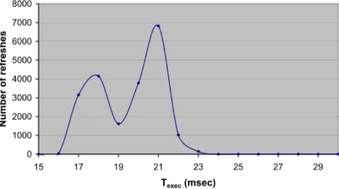
secret. In Figure 6 it is possible to observe the distribution of the (65535) execution times of the experi-ment in the configuration with 6 machines and k = 1. In terms of probability distribution it is clear that the probability of execution time values above 24 msec is low.
The next step was to evaluate the impact of increasing k. Notice that increasing k means that one is attempting to resist a stronger adversary, in other words, resisting the disclosure of a higher number of shares. Therefore, in the second experiment, 6 machines were used to test the behavior of the system with
k varying between 1 and 5. The results are presented in Figure 7. One can see that there is an increment
in the mean and maximum execution when k increases. This increment is also visible in the execution time distribution depicted in Figure 8 and it happens because the size of k impacts the processing delay. Nevertheless, the maximum execution time for k = 5 remains still under 30 ms. This means that one can extend the previous conclusions and say that an adversary would have to obtain 6 shares in less than 2.1 seconds in order to discover the secret.
n Texec(msec)
mean std dev. min, max 2 11.4 3.4 10.0, 20.0 3 15.0 3.1 10.1, 22.3 4 17.0 2.6 10.8, 22.3 5 18.1 2.3 11.3, 23.0 6 19.0 1.5 15.4, 22.8 Figure 5: refresh share execution time with
k = 1 (n – number of machines).
Refresh Duration Distribution 6 mach, 10 ms, k=1, 32 bits 0 1000 2000 3000 4000 5000 6000 7000 8000 15 17 19 21 23 25 27 29 Texec (msec) Number of refreshes
Figure 6: refresh share execution time distribution with 6 machines and k = 1.
k Texec(msec)
mean std dev. min, max 1 19.0 1.5 15.4, 22.8 2 19.8 1.9 12.7, 24.1 3 20.6 2.0 14.6, 25.4 4 21.3 2.3 14.2, 26.4 5 22.6 2.4 14.8, 27.4 Figure 7: refresh shareexecution time with 6 machines.
Refresh Duration Distribution 6 mach, 10 ms, k=5, 32 bits 0 5000 10000 15000 20000 25000 15 17 19 21 23 25 27 29 Texec (msec) Number of refreshes
Figure 8: refresh share execution time distribution with 6 machines and k = 5.
Depending on the assumed adversary strength and on the desired overhead, the system architect can use the above results to calculate the appropriate degree of fault-tolerance k and the values of TP, TDand
Tπ. To illustrate how can this be done, two different adversary types (Hare and Tortoise) are presented
next, and it is described how to configure an appropriate PSSW in each scenario. In both scenarios the system is deployed with 6 machines.
Hare This adversary is able to compromise any machine (i.e., disclose a single share) in one second.
Such an adversary can be envisaged in the context of ultra-resilient systems (e.g., national security related) defending against fierce cyber-attacks.
Without proactive secret sharing, Hare would take k + 1 seconds to discover k + 1 shares and reconstruct the secret. With 6 machines and k = 5, this would mean that the system could be compromised after 6 seconds.