Conservation Biogeography of Amphibians in Mauritania: integrating DNA Barcoding and spatial analyses for the identification of cryptic diversity and phylogenetic units

(1)

of Amphibians in Mauritania:

integrating DNA barcoding

and spatial analyses

for the identification of

cryptic diversity and

phylogenetic units

Ana Marta Martinho Sampaio

Mestrado em Biodiversidade, Genética e Evolução

Departamento de Biologia 2016/2017

Orientador

José Carlos Brito, Investigador Principal, CIBIO

Coorientador

(2)

O Presidente do Júri,

(3)

(4)

To my beloved parents, Ana and Luís.

(5)

(6)

Acknowledgments

To the best supervising duo, José Carlos Brito and Guillermo Velo-Antón, cheers! It was an immense pleasure to work with two creative and committed researchers. I felt supported at every step of the process. I hope both of you see your work recognized and valued as it should. I wish you nothing but the very best.

To the CTM members and all the ones who gave me precious tips for grasping the ghost from the underworld of lab work: Susana Lopes, Diana Castro, Jolita Dilyte, Joana Veríssimo, particularly Patrícia Ribeiro and Sofia Mourão who for sure have a spot reserved in heaven.

Thank you, Filipa Martins, for shedding some light when it came to genetics. Years later, it’s great fun to see how much you’ve grown! I’m grateful to you and Cris for your immense hospitality during my early times in the Far North.

To Wolfgang Böhme and Alberto Sánchez-Vialas who contributed with samples. Thank you, Alberto, for the 48-hour taxonomic marathon.

To BIODESERTS, for all the incredible field and lab work that preceded this thesis and made this work possible. It has been a pleasure.

To all the people out there who create and maintain free servers and software for strangers like me to use, my sincerest acknowledgements. To Alexandra Elbakyan for founding and struggling to maintain the invaluable source of information that is Sci-Hub.

To my Porto crew:

My flatmates and dearest friends, Claudia Chickpea Meneghesso and Fermin Boludo Otero, you filled my heart with joy during my stay in Porto. With you I laughed the perfect laughter. Thank you for taking such good care of me.

Fleur Van deVille, for the tasty homemade warming meals and sweet sharing of stories, concerns and laughers.

Miss Buchadas, apart from the coolest surname ever, you were my partner in crime for almost two years of holy moments. Thank you for the complicity. Thank you for Tarkovsky.

(7)

To my role models, who also happen to be my beloved friends. Andreia Penado, Ricardo Rocha, Diana Rodrigues, Filipa Machado, Cátia Caeiro, Inês Silva, Nídia Fernandes, Aurora Santos, Maggie Wood, Nahla Mahmoud, Ana Bontorim and Ipek Ozdemir I’ve been seeing you all blossoming into outstanding, strong, ethical-driven, genuine individuals. When I grow up I want to carry bits of you with me.

To Teresa Franco and Tiago Jorge, the guardians of my memories, we will get old together either you want it or not.

Thank you, family. Thank you, Salomé, although you still don’t understand it.

Funding for the collection of the samples used in the current M.Sc. thesis were provided by National Geographic Society (grants CRE-7629-04, CRE-8412-08, GEFNE-53-12), Mohammed bin Zayed Species Conservation Fund (grants 11052709, 11052707, 11052499, 13257467), Rufford Foundation (SG-15399-1), Fundação para a Ciência e Tecnologia (PTDC/BIA-BEC/099934/2008, PTDC/BIA-BIC/2903/2012), and FEDER through COMPETE Operational Programme for Competitiveness Factors (FCOMP-01-0124-FEDER-008917, FCOMP-01-0124-FEDER -028276).

(8)

Resumo

A biogeografia da conservação é uma disciplina que recorre a conceitos teóricos e a metodologias da biogeografia para responder a questões conservacionistas, o que lhe concede potencial para combater duas grandes lacunas de conhecimento da biodiversidade, denominadas em inglês, Linnaean shortfall e Wallacean shortfall. A primeira caracteriza o desfasamento que entre a diversidade que realmente existe e a que está formalmente descrita, enquanto que a segunda denota a escassez de conhecimento sobre a geografia da vida. O presente estudo tem como objetivo reduzir estas lacunas de conhecimento nos anfíbios na região de transição biogeográfica da Mauritânia. Utilizam-se dados resultantes do barcoding de ADN e da modelação ecológica espacial para responder às seguintes questões: 1) Quanta diversidade de anfíbios está presente na Mauritânia? 2) Como está essa diversidade geograficamente distribuída? 3) Quais os fatores ambientais que se correlacionam com a distribuição da diversidade de anfíbios? e 4) Onde estão localizados os corpos de água prioritários para a conservação dos anfíbios?

Ao contrário da maioria dos estudos de barcoding em animais que se focam exclusivamente no marcador mitocondrial COI, adicionou-se uma segunda linha de evidência independente com o marcador RAG1 e identificámos 15 taxa. Registaram-se 14 taxa formalmente descritos com presença na Mauritânia e detetou-se potencial diversidade críptica em Hoplobatrachus occipitalis que revelou elevada diversidade intraespecífica. Destaca-se o primeiro registo para a Mauritânia, de dois novos géneros (Amnirana e Leptopelis) e duas novas espécies (Kassina fusca e Tomopterna

milletihorsini). Construiu-se a primeira base de dados de barcoding para os anfíbios da

Mauritânia a partir de 418 indivíduos sequenciados. Identificaram-se seis fatores ambientais correlacionados com a distribuição da riqueza de anfíbios, proximidade à savana e às zonas de várzea de cascalho e distanciamento das dunas e das várzeas de cascalho arenoso. Ao contrário das águas temporárias, as águas permanentes correlacionaram-se negativamente com a riqueza de anfíbios. Os resultados obtidos sublinham a importância dos habitats terrestres e da rede hidrográfica sazonal na manutenção da diversidade de anfíbios na Mauritânia. De acordo com o modelo ecológico, a riqueza de anfíbios segue um gradiente latitudinal, aumentando em direção ao sul, com localidades variando entre zero e 13 taxa. Dois pontos quentes (hotspots em inglês) de biodiversidade foram detetados no sudeste da Mauritânia, numa área rica em zonas húmidas. No entanto, estas zonas ricas em diversidade têm sido substituídas por agricultura, estão desprotegidas, e não estão contempladas na

(9)

rede de espaços protegidos atualmente em discussão para implementação na Mauritânia.

Este estudo oferece uma primeira avaliação da diversidade de anfíbios na Mauritânia e destaca o uso do barcoding de ADN para inferência de padrões biogeográficos à escala regional.

Palavras-chave: anfíbios, barcoding, biogeografia da conservação, diversidade críptica, modelação ecológica, Linnaean shortfall, RAG1, Saara, Sahel, SIG,

(10)

Abstract

By borrowing theoretical and methodological frameworks from biogeography to solve conservation problems, conservation biogeography holds the potential for challenging two major knowledge gaps in biodiversity: the Linnaean and the Wallacean shortfalls. The first stands for the mismatch between the existing and the formally described diversity whilst the second denotes the missing information on the geography of life. The present study aimed at reducing these knowledge shortfalls in the amphibians occurring in the biogeographic transition zone in Mauritania. Data derived from DNA barcoding and ecological spatial modelling were combined for addressing the following questions: 1) How much amphibian diversity is present in Mauritania? 2) How is this diversity geographically distributed? 3) Which environmental factors correlate with amphibian diversity distribution? and 4) Where are priority water-bodies for the conservation of amphibian diversity located?

Unlike in most animal barcoding studies narrowed to the mitochondrial COI, a second independent line of evidence from the nuclear marker RAG1 was added and identified a total of 15 taxa. Fourteen formally described taxa were registered and potential cryptic diversity was detected in Hoplobatrachus occipitalis which displayed high levels of intraspecific diversity. This thesis provides the first record for Mauritania of two new genera (Amnirana and Leptopelis) and two new species (Kassina fusca and

Tomopterna milletihorsini). The first DNA barcoding library for amphibians of Mauritania

was constructed from 418 sequenced individuals. Six environmental correlates of amphibian richness distribution were identified, proximity to savannah and gravel floodplains, and greater distances to yellow dunes and gravel and sand floodplains. Permanent waters related negatively with amphibian richness as opposed to seasonal waters. Results obtained highlighted the importance of a suitable terrestrial habitat and an ephemeral hydrographic network for sustaining amphibian diversity in Mauritania. According to the predictive ecological model, amphibian richness increases southwards following a latitudinal gradient ranging from zero to 13 co-existing taxa per locality. Two major diversity hotspots were detected in south-eastern Mauritania, in a wetland-rich area. Yet, these biodiverse regions have been giving way to agriculture, and no protected areas are implemented nor are they under discussion for implementation in these areas.

This study provides a preliminary assessment of amphibian diversity in Mauritania and highlights the use of DNA barcoding to infer biogeographic patterns at a regional scale.

(11)

Keywords: amphibians, barcoding, conservation biogeography, cryptic diversity, ecological modelling, GIS, Linnaean shortfall, RAG1, transition zone, Sahara, Sahel, Wallacean shortfall

(12)

Table index

Table 1. List of amphibian species recorded in Mauritania, their distribution and population status ... 122 Table 2. Environmental variables used for developing ecological models of amphibian richness distribution in Mauritania. ... 22 Table 3. Summary statistics of uncorrected pairwise distances within species and genera in COI and RAG1 ... 28 Table 4. Coefficient values for all the predictors returned by the final model and cross-validation process relating amphibian richness with environmental predictors in Mauritania ... 35 Supplementary Table 1. Amphibian samples amplified for at least one marker. ……68 Supplementary Table 2. Amphibian samples retrieved from GenBank for both markers... 82 Supplementary Table 3. Correlation matrix between the 12 environmental variables. ... 83 Supplementary Table 4. Support values for clusters obtained from GMYC single-threshold method applied to COI and RAG1 gene trees.. ... 855

(15)

Figure index

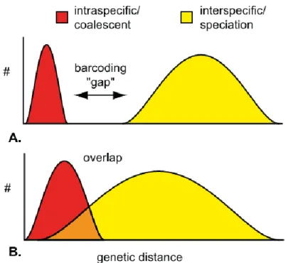
Figure 1. Schematic representation of DNA barcoding gap (Meyer & Paulay, 2005). Intraspecific and interspecific variability are shown in red and yellow, respectively. (A) Discrete distributions without overlap, showing a barcoding gap. (B) Discrete distributions significantly overlapping. ... 4 Figure 2. Predictive model building process (Guisan & Zimmermann, 2000). ... 6 Figure 3. Transition zone in Mauritania. Geographic context of the extent of Sahara and Sahel ecoregions in Africa. Distribution of the montane systems and transition between Sahara and Sahel in Mauritania. ... 9 Figure 4. Distribution of the montane systems and hydrographic network in the study area. ... 15 Figure 5. Study area depicting 61 sampling stations, 36 observation point localities and 418 sequenced individuals from 150 point localities. ... 16 Figure 6. Identified and nonidentified taxa sampled... 17 Figure 7. Distribution of random absences relative to the sampling stations across the study area. ... 23 Figure 8. Phylogenetic reconstruction inferred from COI extended dataset I including sequences from GenBank (family names in grey). ... 25 Figure 9. Phylogenetic reconstruction inferred from RAG1 extended dataset I including sequences from GenBank (family names in grey). ... 26 Figure 10. Phylogenetic reconstruction inferred from COI and RAG extended datasets I including sequences from GenBank (family names in grey). ... 27 Figure 11. Line-plot of the barcoding gap for the 163 COI haplotypes. ... 29 Figure 12. Line-plot of the barcoding gap for the 163 COI haplotypes after splitting H.

occipitalis in two clusters. ... 29

Figure 13. Line-plot of the barcoding gap for the 127 RAG1 haplotypes. ... 30 Figure 14. Line-plot of the barcoding gap for the 127 RAG1 haplotypes after splitting H.

occipitalis in two clusters. ... 30

Figure 15. Phylogenetic reconstruction inferred from COI and RAG1 sequences for Mauritanian amphibians. ... 32 Figure 16. Study area depicting species richness recorded in all sampling stations. .. 33 Figure 17. Predictors from the final model originated by data dredging and its relationship with the observed amphibian richness. R2_{is shown. ... 34}

Figure 18. Predictive accuracy of the chosen model assessed by cross-validation. Relationship between predicted and observed amphibian richness returned by training

(16)

and validation subsets in ten replicates. Lines fitted by simple regression and respective R2 _{values are shown. ... 36}

Figure 19. Amphibian richness map of Mauritania and inset maps showing in detail: (A) Ngouye Classified Forest where the highest observed richness (8 species). (B) Detail of the Kolimbiné river floodplains with high predicted richness (C) Detail of Nioût river floodplains with high predicted richness. (D) Relationship between observed values and model predictions. R2 _{is shown. ... 38}

Supplementary Figure 1. Latest phylogenetic reconstruction for extant amphibians. Maximum likelihood tree built from 2781 species. Adapted from Pyron & Wiens, 2011………...81 Supplementary Figure 2. Spatial variation of the environmental variables in the study area ... 84

(17)

Abbreviation index

AICc – corrected Akaike Information Criterion ANN – Artificial Neural Network

bp – base pairs

BEAST – Bayesian Evolutionary Analysis Sampling Trees BIC – Bayesian Information Criterion

BIN –Barcode Index Number

BLAST – Basic Local Alignment Search Tool BOLD – Barcode of Life Data Systems BRT – Boosted Regression Trees

CBOL – Consortium for the Barcode of Life

CIPRES – Cyberinfrastructure for Phylogenetic Research

CITES – Convention on International Trade in Endangered Species of Wild Fauna and Flora

COI – Cytochrome C oxidase subunit I dd – double-distilled

DEM – Digital Elevation Model ESS – Effective Sample Size GEM – General Ecosystem Model GIS – Geographical Information System GMYC – Generalized Mixed Yule Coalescent GLM – Generalized Linear Model

iBOL – International Barcode of Life

IUCN – International Union for Conservation of Nature MaxEnt –Maximum Entropy

MCMC – Markov Chain Monte Carlo

MNDWI – Modified Normalised Difference Water Index mPTP – Multi-rate Poisson Tree Processes

NDWI – Normalised Difference Water Index NUMT – Nuclear mitochondrial pseudogene PSC – Phylogenetic Species Concept RAG1 – Recombination activating gene 1 SPIDER – Species Identity and Evolution in R SPLITS – Species’ Limits by Threshold Statistics TRI – Terrain Ruggedness Index

(18)

1. Introduction

1.1 Conservation biogeography

Conservation biogeography is a blossoming field aimed at addressing conservation concerns under the study of the dynamics of taxa diversity distribution (Richardson, 2012; Whittaker et al., 2005). This field has recently been substantially boosted by the advent of technical advances in Geographical Information System (GIS) data generation and analysis, and molecular biology (Dawson et al., 2016). These approaches allow investigating spatial patterns (e.g. GIS based modelling of species distributions) and historical processes of biological units, which can be objectively defined (Funk et al., 2012) and subsequently their past, present and future distributions more accurately predicted. Overall, researchers can quantitatively address which species are significantly threatened by extinction, and thereby evaluate conservation measures (Richardson, 2012; Whittaker et al., 2005).

Conservation biogeographers are now equipped with an remarkable set of tools, but our knowledge on biodiversity is still plagued by inadequacies and gaps that bias the available data for accurately describing and predicting its distributional patterns (Hortal et al., 2015). Reducing such bias is of paramount importance for monitoring the biological effects of global change in the midst of an increasing extinction rate (Dirzo et al., 2014; Hortal et al., 2015; Stuart, 2004; Whittaker et al., 2005), so conservation actions can be executed where and when deemed necessary and appropriate. Among several key shortfalls in biodiversity data knowledge, two are the scope of conservation biogeography (Hortal et al., 2015; Whittaker et al., 2005). The Linnaean shortfall denotes the discrepancy between the numbers of species that actually exist and those yet to be formally described and catalogued (Brown & Lomolino, 1998). Although first and foremost a systematics enterprise, conservation biogeography is hampered by our very little understanding of the diversity itself, adding to the biased knowledge on the geography of living organisms, dubbed Wallacean shortfall (Lomolino, 2004). Technical developments are allowing the scientific community to accelerate the collection of data. The following sections aim at introducing two methodological approaches that can challenge these shortfalls.

1.1.1. Linnaean shortfall – DNA barcoding

DNA barcoding emerges as a quick and cost-effective method for specimen’s identification and aiding species discovery, thereby reducing the magnitude of the

(19)

Linnean shortall. It uses molecular markers to amplify short and highly variable DNA sequences (DNA barcode) from standardized regions of the genome, that identify each living organism (Hebert et al., 2003a). The idea was introduced in 2003 by Hebert and colleagues and proposed as a global method to identify animal species by creating cytochrome C oxidase subunit I (COI) profiles out of a ca. 650 bp fragment (Hebert et al., 2003a). The 5´ COI region was demonstrated to be sufficiently conserved within species while variable enough between them to provide for an accurate discrimination of most organisms (Hebert et al., 2003a, 2003b). Despite the fact that DNA barcoding advocated from the early beginning for the use of a global standard fragment, surrogate markers have been developed for many organisms where COI lacks resolution, particularly in plants, protists and fungi (Hajibabaei et al., 2007).

DNA barcoding was also envisioned as part of a solution to overcome a decline of taxonomic expertise, increase the chances of dealing with morphological misidentifications, and resolve adult and larval stages within species (Hebert et al., 2003a). It is tackling the paucity of information in lesser known taxa, such as in marine crustaceans (Raupach et al., 2015), millipedes (Wesener & Conrad, 2016) algae (Leliaert et al., 2014), and fungi (Yahr et al., 2016). From a conservation perspective, it holds the potential for flagging endemic (Hosein et al., 2017) and cryptic diversity (Dincă, et al., 2011; Vasconcelos et al., 2016). It became the new method for the global inventory of life and continues to generate a growing body of literature (Hebert et al., 2016) as well as a substantial media coverage (Geary et al., 2016). Moreover, it became a tool for implementing citizen science and motivating students to pursue STEAM (science, technology, engineering, arts and mathematics) related careers (Henter et al., 2016).

Its growing importance has led to the establishment of worldwide barcoding initiatives, such as the Cold Code (Murphy et al., 2013), a plan for barcoding amphibians and reptiles established under the umbrella of International Barcode of Life (iBOL) project [http://www.ibol.org]. iBOL works in collaboration with citizens, organisations and researchers around the world to build a publicly searchable comprehensive databank of DNA barcodes dubbed BOLD (Ratnasingham & Hebert, 2007) – Barcode of Life Data Systems [http://www.boldsystems.org]. Institutions investing in DNA barcoding can also join the Consortium for the Barcode of Life (CBOL) aimed at promoting and developing DNA barcoding through workshops, networks, conferences and training [http://www.barcodeoflife.org]. BOLD harbours DNA barcode reference libraries that are built from identified and vouchered specimens and aim at ensuring reproducibility, traceability and reliability of the taxonomic process (Hubert & Hanner, 2015;

(20)

Ratnasingham & Hebert, 2007). It also provides a workbench for analytical procedures (Ratnasingham & Hebert, 2007). A pipeline has also been developed to cluster DNA sequences of closely related species deposited in BOLD into BINs (Barcode Index Numbers) for the entire animal kingdom (Ratnasingham & Hebert, 2013). A sample ID number and a taxonomic assignment are required to submit new sequences, but records must meet specific requirements to achieve a formal barcode status such as possessing a minimum length of 500 bp in the case of COI (Ratnasingham & Hebert, 2007).

At the heart of the DNA barcoding lies the assumption that a barcoding gap exists between two ranges of genetic variation: intraspecific polymorphism and interspecific divergence (Figure 1) (Hebert et al., 2003a, 2003b, 2004; Meyer & Paulay, 2005). In other words, the greatest intraspecific genetic distance will be lower than the smallest interspecific genetic distance. As such, accuracy, performance of a given barcode in discriminating species, will depend largely on the separation and extent of these two ranges of variability in the molecular marker (Meyer & Paulay, 2005). After retrieving the barcode from the specimen, its accuracy should be measured by comparing the query sequence to a comprehensive molecular databank in order to assign the unknown sampled specimen to a known species (Ratnasingham & Hebert, 2007). Because these reference libraries are still inexistent for most species, a plethora of methodological strategies are being employed/developed to accurately identify specimens and to assist species discovery: distance-based (Aliabadian et al., 2009; Vasconcelos et al., 2016), phylogeny-based (Vasconcelos et al., 2016), diagnostic (DasGupta et al., 2005) and statistical (Nielsen et al., 2006). Associated to these, species delimitation methods are commonly used in barcoding studies (Talavera et al., 2013; Zhang et al., 2013a).

However, in incipient species that have not been yet fully separated by the coalescent, these two ranges of variability can overlap (Rosenberg, 2003) and therefore, no barcoding gap would be observed (Figure 1). Moreover, cases of paraphyly and polyphyly may arise due to hybridisation, introgression and incomplete lineage sorting following recent speciation (Funk & Omland, 2003), which introduces complexities when attempting to differentiate species through barcoding techniques since phylogeny-based methods require reciprocal monophyly. Absence of a barcoding gap, or reciprocal monophyly, can likewise result from misidentification (Mutanen et al., 2016), inaccurate reference taxonomy (Mutanen et al., 2016) undersampling (Meyer & Paulay, 2005) or presence of cryptic species (Mutanen et al., 2016).

(21)

Figure 1. Schematic representation of DNA barcoding gap (Meyer & Paulay, 2005). Intraspecific and interspecific

variability are shown in red and yellow, respectively. (A) Discrete distributions without overlap, showing a barcoding gap. (B) Discrete distributions significantly overlapping.

Researchers are now beginning to extend the number of independent molecular markers in DNA barcoding studies (Dupont et al., 2016; Simeone et al., 2013) allowing to tackle non-reciprocal monophyly issues (Funk & Omland, 2003; Vences et al., 2005a) and to move away from one of the major shortcomings of earlier barcoding studies, the assumption that gene trees and species trees are identical (Degnan & Rosenberg, 2009; Mallo & Posada, 2016).

From identifying singles specimens, DNA barcoding evolved to identifying entire communities through high-throughput DNA sequencing from mass collections of organisms or from environmental DNA, a technique called metabarcoding (Taberlet et al., 2012). Since metabarcoding demands a considerable investment to build high quality reference libraries, standard DNA barcoding and databases like iBOL with well-curated collections of specimens, still often offer the best solution for species identification in metabarcoding studies (Taberlet et al., 2012). The research community currently uses DNA barcoding and metabarcoding approaches in numerous ecological studies that go beyond taxonomy and biodiversity inventories, often revealing conservation and socio-economic applications (Adamowicz, 2015). Examples include border biosecurity such as detection of regulated pests (Hodgetts et al., 2016) and

(22)

invasive organisms (Armstrong & Ball, 2005), exposing and controlling illegal trade of CITES species (Williamson et al., 2016) and unregulated fishing (Helyar et al., 2014), study of food webs structure (McLean et al., 2016; Roslin et al., 2016; Smith et al., 2011), characterization of host-associated communities (Baker et al., 2016), and authentication of medicinal plants (Chen et al., 2014).

1.1.2. Wallacean shortfall – spatial ecological modelling

Ecological spatial modelling is a mathematical modelling approach for understanding, predicting (current conditions) and forecasting (future conditions) ecological relationships in a geographical space, based on GIS and/or remote sensing data (Jørgensen & Fath, 2011). It helps disentangling biodiversity spatial patterns at different grain sizes (e.g. Brito et al., 2016; Vale et al., 2015) and allows to generate information on species occurrence data at a fine spatial grain otherwise hard to obtain and essential for informing conservation action (Jetz et al., 2012). In this regard, spatial ecological modelling offers a powerful tool for conservation biogeography to reduce the Wallacean shortfall.

As simplified versions of a complex reality, ecological mathematical models were borrowed from physical systems to synthetize our knowledge on the natural world (Jørgensen & Bendoricchio, 2001). They were first boosted by the increasing power of computer tools and later matured with the inclusion of fixed modelling procedures and more ecological knowledge (Jørgensen & Bendoricchio, 2001). Since then, different statistical and computational frameworks have been developed to grasp the overwhelming complexity of ecosystems in many different subfields of ecology and environmental management (Jørgensen & Fath, 2011). Spatial modelling has been profiting from these advances by incorporating a variety of techniques with examples including Artificial Neural Networks (ANN; Fischer, 2006), Generalized Linear Models (GLM) and extensions (Guisan et al., 2002), Maximum Entropy (MaxEnt; Phillips et al., 2006), Boosted Regression Trees (BRT; Friedman, 2001) and General Ecosystem Model (GEM; Harfoot et al., 2014).

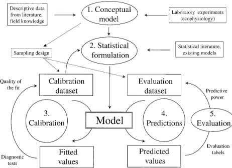
Building a predictive spatial model begins with the identification of a problem or a natural system (Jørgensen & Fath, 2011) and, depending on the author, can be summarized in five major steps as schematised in Figure 2: (1) conceptual model, (2) statistical formulation, (3) calibration, (4) predictions and (5) evaluation.

(23)

Figure 2. Predictive model building process (Guisan & Zimmermann, 2000).

Conceptualization begins by laying a theoretical framework regarding the general patterns in the distribution of organisms (Guisan & Zimmermann, 2000). Then, it follows the choice on whether describing an empirical correlation (correlative models) or a causal link (mechanistic models) between two or more ecological variables. This stage implies understanding the trade-offs between the reality, precision and transferability (generalization) of the model’s predictive ability (Guisan & Zimmermann, 2000). An important part of the conceptualization step involves defining what to model: individual species and lineages (e.g. Rosauer et al., 2015) or properties of entire communities (Ferrier & Guisan, 2006). When modelling properties of communities, such as species richness, three distinct approaches can be considered: “assemble first, predict later” in which richness is estimated directly using predictors; “predict first, assemble later” in which richness is estimated from modelled species’ distributions; and “assemble and predict together” that implies modelling all species simultaneously (Ferrier & Guisan, 2006). Conceptualization ends with a set of meaningful predictive variables and an appropriate spatial scale (Guisan & Zimmermann, 2000). Ideally, the conceptual model should determine the collection of the data, but in reality, models are often developed from available data due to logistic and economic limitations (Jørgensen & Fath, 2011).

The second step of the model building process leads to the translation of our knowledge on a natural system into a mathematical formula, through the selection of an optimal statistical approach (Guisan & Zimmermann, 2000).

(24)

The third step involves fitting the model to the data by comparing its output (prediction values) to the observations. It is aimed at increasing the predictive power and accuracy of the model. The initial set of predictors is often downsized which can be done automatically, for instance, through data dredging (Barton, 2016).

So far, we have acquired an understanding of a certain natural system and formalized it as a model, that can be used for making predictions of current conditions. In spatial modelling, the forth step involves predicting the distribution of living organisms within the modelled area which can then, be mapped, for instance, by implementing the model in a GIS environment (Guisan & Zimmermann, 2000).

The model building process ends with a final validation step aimed at evaluating the predictive power of the model, for example, through cross-validation. In other words, the goal is not to test if a model is true or false, but to confirm its behaviour under a range of conditions represented by the data (Guisan & Zimmermann, 2000).

Ecological spatial modelling has been used by both the research community and conservation practitioners to deal with a vast array of topics like invasive biology (Buchadas et al., 2017), climate change research (Penado et al., 2016), landscape connectivity (Roscioni et al., 2014), human-wildlife conflicts (Braunisch et al., 2011; Roscioni et al., 2014), ecological succession (Mittanck et al., 2014) and ecosystem services (Nelson et al., 2009).

1.2. Biodiversity in arid regions

With extreme aridity indices (annual precipitation/potential evapotranspiration rates) falling below 0.20 and subjected to infrequent and intense pulses of precipitation (Ward, 2016), warm deserts and arid regions are harsh abiotic environments that push nature into unique adaptations to climate extremes (Brito et al., 2014). Precisely because of the possibility of already inhabiting close to physiological limits, desert-adapted species might be more strongly impacted by climate change (Vale & Brito, 2015). A scenario that is aggravated by the high vulnerability of drylands to global environmental changes (IPCC, 2014; Loarie et al., 2009).

Among all arid regions, the Sahara-Sahel stands out with a set of idiosyncrasies potentially leading to cryptic diversity and localised biodiversity hotspots (Brito et al., 2014) critical for conservation (Brito et al., 2016; Vale et al., 2015). The boundary between the Sahara and the Sahel is situated in a crossroad between the Palaearctic and Afro-tropic terrestrial biogeographical realms (Dinerstein et al., 2017), thereby

(25)

comprising several distinct terrestrial ecosystems and phytogeographic regions (Sayre et al., 2013). This transition translates into high levels of species richness as expected whenever areas with distinct important biodiversity elements intersect (Spector, 2002). The Sahara-Sahel spreads over 10 countries that have been staging political and socio-economic instability in different degrees, often associated to terrorism (IEP, 2016). Besides the obvious tragic consequences for local populations that largely live in low human development (UNDP, 2016), the current situation is having a pervasive impact on wildlife and hampering basic scientific research (Brito et al., 2014; Durant et al., 2012).

1.2.1. The transition zone in Mauritania

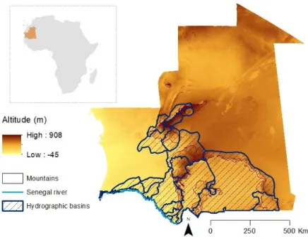
Mauritania lies in the transition zone between the Palaearctic and Afro-tropic realms. A system of mountains and plateaux with associated water-bodies surrounded by sand seas, typically punctuates the landscape (Brito et al., 2016; Le Houérou, 1997). Four major massifs, Adrar Atar in the Sahara, Tagant, Assaba and Afollé in the Sahel, constitute the mountain system of the country (Figure 3). Predominantly in the Saharan desert, these water-bodies occur essentially seasonally and isolated in the form of small mountain rocky pools locally known as gueltas (between 0.001 and 1.0ha) (Campos et al., 2012; Cooper et al., 2006). They are typically deep, located upstream mountain valleys and supplied by torrential rains during the short raining season between July and September (Brito et al., 2011; Cooper et al., 2006). As we move further south into the Sahel, the hydrographic network begins to be increasingly connected; riverbeds (wadis) and floodplains (tâmoûrts) become more common (Campos et al., 2012). Tâmoûrts form at the foothills of massifs, are more shallow than

gueltas and therefore tend to dry outside the rainy season (Cooper et al., 2006), and

are supplied by the wadis formed during torrential rainfalls (Campos et al., 2012). The region also displays a latitudinal variation in the species distribution patterns. The diversity of both fauna and flora is widespread in the south and increasingly confined and scattered towards north (Brito et al., 2014; Le Houérou, 1997). Mountains and associated hydrographic sub-basins (Figure 4) form localised biodiversity hotspots, where both endemic and relict taxa with several biogeographic affinities occur (Brito et al., 2014). Adrar Atar and Tagant are particularly rich, with the former hosting the highest number of Saharan vertebrate endemics (Brito et al., 2014). Particularly in the Sahara, many water dependent species persist in isolated populations within restricted habitats, mainly associated to gueltas that constitute refugia for both endemic and

(26)

range-limit populations (Brito et al., 2011, 2014; Trape, 2009; Vale et al., 2015; Velo-Antón et al., 2014) and where cryptic diversity is being uncovered (Brito et al., 2016). The Mauritanian hydrographic network has been suggested to play a crucial role for the persistence of crocodile (Crocodylus suchus) populations in the region, by allowing dispersal movements along the wadis connecting populations otherwise completely isolated (Velo-Antón et al., 2014). Extreme temperatures and droughts coupled with human disturbance are threatening these inland waters, yet, 80% of the gueltas identified as priority for conservation in Mauritania do not hold any legal protection status (Vale et al., 2015). Moreover, facing an accelerating water cycle, where wet areas become wetter and dry areas become drier (Sutherland et al., 2013), the Sahel is expected to experience amongst the highest drought recovery times of the planet (Schwalm et al., 2017). Species loss could, therefore, be more acute than hypothesized (Sutherland et al., 2013).

Figure 3. Transition zone in Mauritania. Geographic context of the extent of Sahara and Sahel ecoregions in Africa.

(27)

1.2.2. Amphibians of Mauritania

Amphibian distribution in Mauritania is widespread in the Sahel but rather restricted in the southern Sahara where population isolates are confined to the wadis, gueltas and springs, with important areas occurring in the mountains and some could temporarily connect during the rainy season (Padial et al., 2013). Because of this distribution pattern, amphibians occurring in the dryer Sahara are hypothesized to result from the dispersion of species coming from the Sahelian savannah. Priority areas for amphibian conservation are thought to be along the hydrographic network on the more explored massifs of Adrar Atar and Tagant (Padial et al., 2013). The last one lies midway between the two realms, exhibiting transitional environmental features and therefore, containing more suitable habitats for amphibians (Padial et al., 2013). On the other hand, the southern less known mountains of Assaba and Afollé, as well as the Senegal river basin might also prove to be equally important (Padial et al., 2013). Gueltas in Assaba recorded so far the highest amphibian richness of all four major massifs associated gueltas (Vale et al., 2015), meaning the unexplored associate river basins and tâmoûrts hold the potential of being equally rich. The undersampled savannah bordering Senegal and Mali in the south of the country is also expected to be diverse (Padial et al., 2013). Data on the distribution and diversity of amphibians of Mauritania has been highlighted as a priority research need for the region (Padial et al., 2013). Yet, only 12 anuran species have been reported in the country (Table 1), with the first record of a newly confirmed species (Ptychadena schillukorum) being from 2017 (Sánchez-Vialas et al., 2017). This suggests an underestimation of the Mauritanian amphibian diversity, and more species are hypothesized to exist given that large southern areas remain unexplored and taxonomy of these species is seldom reliable (Padial et al., 2013).

Only three species have been recorded across the Saharan realm: Hoplobatrachus

occipitalis, Sclerophrys xeros, and Tomopterna cryptotis (Table 1). Further south, the

Sahel exhibits higher diversity and comprises all species present in the Sahara (Padial et al., 2013). Among the true toads, family Bufonidae, three species belonging to genus

Sclerophrys are known to occur in Mauritania. Potential breeding sites of S. regularis

include a vast variety of water-bodies, from permanent to temporary, from lotic to lentic water systems (Rödel, 2000). Reproduction in S. xeros and S. pentoni seems to be more associated to ponds instead (Rödel, 2000). H. occipitalis from the Dicroglossidae family, is essentially an aquatic species; its tadpoles are capable of surviving in shallow ponds at high temperatures and can prey on S. xeros tadpoles (Rödel, 2000). The ground-dwelling Kassina senegalensis is the sole representative of the hyper diverse

(28)

clade Afrobatrachia and so far, breeding is known to occur in lentic systems (Fleischack & Small, 1978). The species rich family of puddle frogs Phrynobatrachidae, counts with records of Phrynobatrachus natalensis, with breeding sites associated to lentic systems, mainly ponds and puddles (Rödel, 2000). Four species from the family Ptychadenidae have been recorded in Mauritania. They belong to the genus

Ptychadena, that comprises species that frequently occur in syntopy (Bwong et al.,

2009; Rödel, 2000) and commonly breed in lentic water-bodies with associated vegetation (Rödel, 2000). The family Pyxicephalidae is represented in Mauritania by two ground-dwelling species, Pyxicephalus edulis and Tomopterna cryptotis, the latter is thought to be mostly nocturnal (Rödel, 2000).

To date, no species hold an unfavourable conservation status (Table 1), yet it could change as knowledge on the Saharan isolates is being gathered.

(29)

Table 1. List of amphibian species recorded in Mauritania, their distribution and population status. Family Species (Rödel, 2000) Species (Padial et al., 2013) Species (IUCN, 2015)

Distribution and Population Status (Padial et al., 2013)

Taxonomic Status

(Rödel, 2000) Notes

Bufonidae Bufo pentoni “Bufo” pentoni Sclerophrys pentoni

Scattered localities across the Sahelian

savannah; locally abundant Stable -

Bufo regularis Amietophrynus

regularis

Sclerophrys regularis

Scattered localities across the Sahelian savannah and along the coast; locally abundant

Unstable; possible

species complex -

Bufo xeros Amietophrynus

xeros

Sclerophrys

xeros Most Saharan waterbodies; locally abundant

Unstable; possible species complex - Dicroglossidae Hoplobatrachus occipitalis Hoplobatrachus occipitalis Hoplobatrachus occipitalis

Most Saharan waterbodies and across the Sahelian savannah; locally abundant but possible local extinctions have occurred

Unstable; possible species complex - Hyperoliidae Kassina senegalensis Kassina senegalensis Kassina senegalensis

Scattered localities across the Sahelian savannah; scarce

Unstable; possible

species complex -

- - Hyperolius

nitidulus - -

Never reported; considered by IUCN as likely in Guidimaka province

Microhylidae - - Phrynomantis

microps - -

Never reported; considered by IUCN as likely in Guidimaka province

Phrynobatrachidae - - Phrynobatrachus

francisci - -

Never reported; considered by IUCN as likely along the Senegal river Phrynobatrachus cf. natalensis Phrynobatrachus natalensis Phrynobatrachus natalensis

Known only from a single locality in the Sahelian savannah; no data on abundance

Unstable; possible

species complex -

Ptychadenidae Ptychadena

bibroni Ptychadena bibroni -

Known from two localities in the Sahelian

savannah; no data on abundance Stable Excluded by IUCN

Ptychadena mascareniensis Ptychadena mascareniensis Ptychadena mascareniensis

Known only from a single locality in the Sahelian savannah; no data on abundance

Unstable; possible

(30)

Family Species (Rödel, 2000) Species (Padial et al., 2013) Species (IUCN, 2015)

Distribution and Population Status (Padial et al., 2013)

Taxonomic Status

(Rödel, 2000) Notes

- - Ptychadena

pumilio - -

Never reported; considered by IUCN as likely along all southern Mauritania Ptychadena trinodis Ptychadena trinodis Ptychadena trinodis

Known from two localities in the Sahelian

savannah; no data on abundance Stable -

Pyxicephalidae Pyxicephalus edulis Pyxicephalus edulis Pyxicephalus edulis

Scattered localities across the Sahelian savannah; probably locally abundant

Unstable; possible species complex - Tomopterna cryptotis Tomopterna cryptotis Tomopterna cryptotis

Scattered localities across the Sahelian savannah; also recorded from the coast and in some Saharan waterbodies; rare

Unstable, possible

(31)

2. Objectives

This study addresses the following questions: 1) How much amphibian diversity is present in Mauritania? 2) How is this diversity geographically distributed? 3) Which environmental factors correlate with amphibian diversity distribution? and 4) Where are priority water-bodies for the conservation of amphibian diversity located? Overall, this study will allow us to conduct a preliminary conservation assessment of Mauritanian amphibians by identifying hotspots of diversity. Our goal is to detect key locations for conservation of autochthonous amphibian species occurring in water-bodies of Mauritania by assessing the environmental correlates of their distributions.

Specifically, we aim to:

(a) Identify amphibian species and possibly cryptic diversity, using two independent genetic markers, the mitochondrial COI and the nuclear RAG1;

(b) Build a barcode library for the region providing a useful and standardized species identification tool, improving the poor taxonomic knowledge of Mauritanian amphibians;

(c) Quantify amphibian richness and assess its distribution patterns; (d) Identify environmental correlates of amphibian richness distribution; (e) Identify diversity hotspots.

This work will contribute directly for building the first DNA barcode library for the amphibian species of the region and for an atlas of the distribution of the herpetofauna of Mauritania.. . . . . . . . . . . .

(32)

3. Methods

3.1. Study area

The study area comprises Mauritania, Northwest of Africa, where tissue samples have been collected from individuals captured along the hydrographic network, in lowlands and mountains (Figure 4). The mountain of Adrar Atar, Tagant, Afollé and Assaba harbour endemic and relict vertebrate and invertebrate taxa (Brito et al., 2014). The central-southern Mauritania lies within the Sahel ecoregion and exhibits increased water availability, which includes the Senegal river in the southern border of the country (Figures 3 and 4; Campos et al., 2012).

Figure 4. Distribution of the montane systems and hydrographic network in the study area.

3.2. Fieldwork

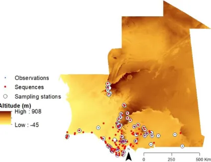
A total of 418 samples were collected by researchers and collaborators of BIODESERTS – Biodiversity of Deserts and Arid Regions – research group during 16 field expeditions between 2003 and 2016 (Appendix: Supplementary Table 1). Amphibians were sampled using dip-nets, from across the Sahara-Sahel. Tissue samples were collected by toe and tail-clipping of adult specimens and tadpoles respectively, and stored them in 95% ethanol. Locality data for all samples was geo-referenced in the field with a Global Positioning System (GPS) on the WGS84 datum. Samples were collected for genetic analyses over 195 point localities, registered observations and collect specimens over 38 point localities (Figure 5). For ecological

(33)

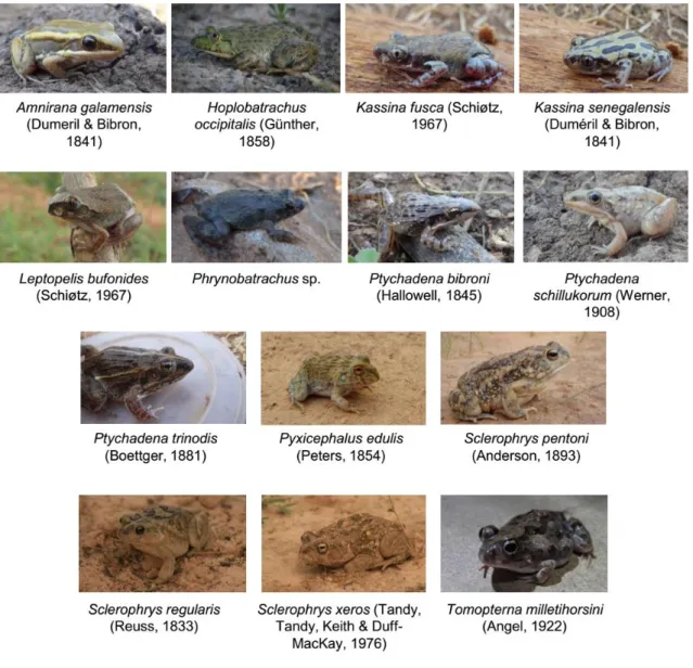
modelling, we used richness values from 61 sampling stations located in Mauritanian selected taking into account a similar sampling effort (Figure 5). Whenever possible, specimens were assigned to formally described species through careful examination of vouchers, photographs and location data. For this purpose, we resorted to taxonomic expertise which allowed for the morphological identification of the diagnostic characters. We followed the latest amphibian phylogenetic reconstruction from Pyron and colleagues (Appendix: Supplementary Figure 1; Pyron & Wiens, 2011) for reference and identified 13 formally described amphibian species plus one identified only at the genus level (Phrynobatrachus sp.) (Figure 6). Our dataset included putatively seven species from five Afro-tropic endemic genera: Kassina (K. fusca and

K. senegalensis) Leptopelis (L. bufonides), Phrynobatrachus sp., Ptychadena (P. bibroni, P. schillukorum and P. trinodis), Pyxicephalus (P. edulis) and Tomopterna (T. milletihorsini) (Frost et al., 2006; Pyron & Wiens, 2011; Stuart et al., 2008).

Non-endemic genera in the Afro-tropics occurring in Mauritania include Hoplobatrachus (H.

occipitalis) (Stuart et al., 2008) and Sclerophrys (S. pentoni, S. regularis and S. xeros)

(Frost, 2017). Amnirana genus is the only member of the essentially Palaearctic family Ranidae occurring in the Afro-tropic realm (Stuart et al., 2008) and is represented in Mauritania by A. galamensis.

Figure 5. Study area depicting 61 sampling stations, 36 observation point localities and 418 sequenced individuals from

(34)

Figure 6. Identified and nonidentified taxa sampled.

3.3. DNA extraction, amplification and sequencing

We performed DNA extraction and purification from tissue samples using Easy Spin extraction and purification kit. We verified the quality and approximate quantity by electrophoresis in TBE (Tris-Borate-EDTA buffer) 0.5x at 300V, using 0.8% agarose gel stained with gel red (Biotium). We then visualised the gel through UV radiation in a BioRad Universal Hood II Quantity One 4.4.0. Whenever necessary, we diluted the extractions by adding ultra-pure water before proceeding to PCR. The COI marker was ampliﬁed using the primer pair Chmf4 (5′-TYT CWA CWA AYC AYA AAG AYA TCG C-3′) and Chmr4 (5′-ACY TCR GGR TGR CCR AAR AAT CA-C-3′) (Che et al., 2012). We selected a second slower evolving marker (San Mauro et al., 2004a), the nuclear recombination-activating gene 1 (RAG1), frequently used in amphibian phylogenetic

(35)

reconstructions and proven to be useful at inter-specific levels (Frost et al., 2006; Hoegg et al., 2004; Irisarri et al., 2012; Portik & Blackburn, 2016; Pyron & Wiens, 2011; Roelants et al., 2007; San Mauro et al., 2004; van der Meijden et al., 2004; Wiens, 2007). RAG1 was amplified using Amp-RAG1 F (5′-AGC TGC AGY CAR TAC CAY AAR ATG TA-3′) and Amp-RAG1 R1 (5′-AAC TCA GCT GCA TTK CCA ATR TCA CA-3′) (San Mauro et al., 2004b). We performed the PCR of both genes in a 10-µl volume reaction containing 1µl of DNA, 3µl of ddH2O, 5µl of Taq polymerase and 0.5µl of each

primer. PCR conditions for COI (a) and RAG1 (b) respectively, were as follows: (a) initial denaturation step with 5 min at 95ºC; 35 cycles of denaturation for 1 min at 94ºC, annealing for 1 min at 52ºC and extension for 1 min at 72ºC; final extension at 72ºC for 10min; (b) initial denaturation step with 5 min at 94 ºC; 35 cycles of denaturation for 1 min at 94ºC, annealing for 1 min at 54ºC and extension for 1.30 min at 72ºC; final extension at 72ºC for 7 min. We confirmed the presence of the PCR products by 2% gel electrophoresis. Purification and Sanger Sequencing protocols of PCR products were outsourced to GeneWiz.

We inspected and verified the sequence chromatograms and alignments using Geneious v.4.8.5 (http://www.geneious.com/; Kearse et al., 2012). Aside from a gap penalty set at 100, we used the default settings of the Geneious alignment algorithm to produce global alignments for each gene. To detect the presence of nuclear mitochondrial pseudogenes (NUMTs), we searched for ambiguities and translated all aligned sequences into amino acids and looked for stop codons and frameshift mutations (Bensasson et al., 2001). RAG1 polymorphic sites were encoded with the IUPAC ambiguity code. We submitted the sequences to a BLAST (Basic Local Alignment Search Tool) in GenBank and BOLD databases, to confirm that the targeted regions had been amplified.

We sequenced all the 418 samples with 606bp for the mitochondrial COI and selected 187 nuclear sequences with 854bp in order to represent all mitochondrial lineages (Appendix: Supplementary Table 1). We identified haplotypes with FaBox v.1.41 (Villesen, 2007) and removed sequences from the subsequent analyses for computational reasons. We then built two datasets for each marker: i) 186 COI and 151 RAG1 haplotypes from samples collected throughout the Sahara-Sahel, herein datasets I, and ii) 163 COI and 127 RAG1 haplotypes from samples collected only in Mauritania, herein datasets II.

(36)

3.4. Phylogenetic reconstruction

We used datasets I and extended it to included 21 species retrieved from GenBank, representing families missing in the study area, following the phylogenetic reconstruction from Pyron and colleagues (Pyron & Wiens, 2011) (Appendix: Supplementary Table 2). The aim was to obtain a better resolved topology, for solving and comparing phylogenetic relationships between species. We employed a Bayesian inference approach implemented in BEAST v.2.4.6 (Bouckaert et al., 2014) provided by CIPRES science gateway v.3.3 (Miller et al., 2010) to construct all trees. We applied the closest nucleotide substitution models available in BEAST as suggested by ModelFinder (Kalyaanamoorthy et al., 2017) implemented in IQ-Tree web server (Trifinopoulos et al., 2016), and selected according to BIC (Bayesian Information Criterion). We diagnosed chains convergence by inspecting the trace plots and effective sample sizes (ESS) of the parameters in Tracer v.1.6 (Rambaut et al., 2003) and combined the trees with LogCombiner 2.4.5 and TreeAnnotator 2.4.5. We used Figtree v.1.4.3 (http://tree.bio.ed.ac.uk/software/figtree/) to visualize and edit consensus trees. As some of the subsequent methods require a corrected rooted tree, we chose Ascaphus truei as an outgroup taxon (Irisarri et al., 2012).

We obtained a gene tree for each marker. We selected the following settings (otherwise by default): COI tree site model TN93+I+G and RAG1 tree site model HKY+I+G; strict clock model; Yule tree prior; ingroup enforced monophyly; MCMC length of 1000 000 000 steps and logging parameters every 10 000 000 step, combining three independent runs and a 10% burn-in.

We ran an analysis with a partitioned dataset including COI and RAG1 haplotypes and selected the following settings (otherwise by default): COI tree site model HKY+I+G and RAG1 tree site model TVMe+I+G; strict clock model; Yule tree prior; ingroup enforced monophyly; MCMC length of 100 000 000 steps and logging parameters every 10 000 000 step, combining three independent runs and a 10% burn-in.

Although not appropriate for inter-species datasets, strict clocks were enforced in these analyses to reach chain convergence.

3.5. Sequence similarity analyses and barcoding gap

The following analyses are implemented in the R (R Core Team, 2017) package SPIDER v.1.3 (Brown et al., 2012) and were run on datasets II. We produced an uncorrected pairwise distance matrix for each marker, following previous recommendations on model choices for constructing matrices from low genetic

(37)

distances (Nei & Kumar, 2000). We then performed two query identification analyses to evaluate the identification performance of our COI barcodes, and to distinguish between successful, ambiguous, misidentified sequences or no match (Meier et al., 2006): Meier's best close match and BOLD identification criteria. Both imply the use of distance thresholds that we defined as 10%, as previously proposed for amphibians (Vences et al., 2005a). Meier's best close match finds the closest individual to the query sequence (Austerlitz et al., 2009; Meier et al., 2006) while BOLD identification criteria emulates the method of specimen identiﬁcation used by BOLD. To evaluate the presence of barcoding gap at species and genus level in both COI and RAG1 datasets, we used the statistics maxInDist (furthest intraspecific distance) and nonConDist (smallest interspecific distance) rather than mean distances which can overestimate it (Meier et al., 2008). If the difference between the furthest intraspecific distance and the smallest interspecific distance results positive, there is a barcoding gap, otherwise it reflects an overlap between the two ranges of distances.

3.6. Delimitation of phylogenetic units

To delimit putative species, we applied single-locus species delimitation methods to the gene trees for identifying discrete genetic clusters, following the phylogenetic species concept (PSC; Eldredge & Cracraft, 1980). We used the Generalized Mixed Yule Coalescent (GMYC) model (Pons et al., 2006) implemented in the R package SPLITS (Ezard et al., 2009), which identifies the transition between a Yule-type speciation (inter-species) and a coalescent (intra-species) branching rates using an ultrametric tree by maximizing the likelihood score of the model (Fujisawa & Barraclough, 2013). We ran GMYC single-threshold as the multiple-threshold approach generally yields a lower taxonomic accuracy (Fujisawa & Barraclough, 2013). We also employed the multi-rate Poisson tree processes (mPTP) model (Kapli et al., 2017) implemented in MPTP Web Server (http://mptp.h-its.org/#/tree; Zhang et al., 2013), which relies on the branch lengths to infer putative species boundaries on a given phylogenetic input tree. Contrary to the previous version, the single-rate Poisson tree processes (PTP) model, it assumes different evolution rates for different species (Kapli et al., 2017; Zhang et al., 2013a).

These methods were applied in single gene trees obtained for each marker from datasets II. We selected the following settings (otherwise by default): COI tree site model TN93+I+G and RAG1 tree site model K2P+G; strict clock model; Yule tree prior; ingroup enforced monophyly; MCMC length of 1000 000 000 steps and logging

(38)

parameters every 10 000 000 step, combining three independent runs and a 10% burn-in.

3.7. Spatial ecological modelling

Using the distinct taxa identified in the precious sections, we applied spatial ecological modelling to identify environmental correlates of amphibian richness distribution, predict its patterns within the study area and finally map the predictions by implementing the model in a GIS environment.

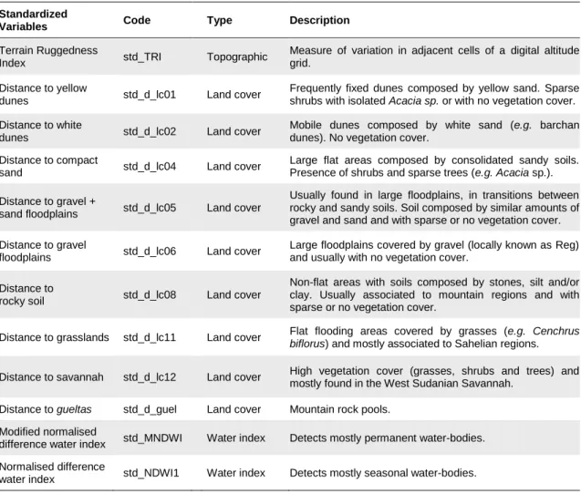
We obtained grid-based datasets for current environmental conditions in the study area comprising topographical variables, land cover types and water indexes. The datasets were downsized to include 12 uncorrelated (R < 7; Appendix: Supplementary Table 3) environmental variables (Table 2; Appendix: Supplementary Figure 2). We applied the

terrain function in R package raster v.2.5-8 in a DEM (Hijmans, 2016) to a Digital

Elevation Model (DEM) to derive the Terrain Ruggedness Index (Riley et al., 1999) with a 90 m resolution. We obtained eight types of land cover with a 30 m resolution from a remote sensing-derived land cover map (Campos et. al. unpublished data): std_d_lc01, std_d_lc02, std_d_lc04, std_d_lc05, std_d_lc06, std_d_lc08, std_d_lc11, std_d_lc12. and std_d_guel. A last land cover variable with 90 m resolution, std_d_guel was obtained from GPS (WGS84 datum) recorded localities and areas during field missions. The water indexes std_MNDWI and std_NDWI1 were derived from remote sensing and had a resolution of 30 m (Campos et al., 2012).

We chose 12 environmental variables according to the spatial auto-correlation coefficients, the spatial scale, the present-day knowledge on the Mauritanian amphibians’ natural history traits and on the regional climate and habitats to avoid overfitting caused by an excess of model parameters. As such, some correlations above 0.7 were allowed, given the likely importance for the distribution of amphibians (Appendix: Supplementary Table 3). To avoid problems caused by negative values and by the differential weight arising from different units of measure, we applied a Min-Max standardization technique to all variables, scaling the data between zero and one: zi =

(xi - minx) / (maxx - minx); where zi denotes the ith normalized data, xi the ith observation,

and maxx and minx the maximum and minimum value respectively. All variables were

upscaled to 90 m and projected in the WGS84 datum. These analyses were performed in ArcMap v.10.1 (ESRI, 2012).

(39)

Table 2. Environmental variables used for developing ecological models of amphibian richness distribution in

Mauritania.

Standardized

Variables Code Type Description

Terrain Ruggedness

Index std_TRI Topographic

Measure of variation in adjacent cells of a digital altitude grid.

Distance to yellow

dunes std_d_lc01 Land cover

Frequently fixed dunes composed by yellow sand. Sparse shrubs with isolated Acacia sp. or with no vegetation cover. Distance to white

dunes std_d_lc02 Land cover

Mobile dunes composed by white sand (e.g. barchan dunes). No vegetation cover.

Distance to compact

sand std_d_lc04 Land cover

Large flat areas composed by consolidated sandy soils. Presence of shrubs and sparse trees (e.g. Acacia sp.). Distance to gravel +

sand floodplains std_d_lc05 Land cover

Usually found in large floodplains, in transitions between rocky and sandy soils. Soil composed by similar amounts of gravel and sand and with sparse or no vegetation cover. Distance to gravel

floodplains std_d_lc06 Land cover

Large floodplains covered by gravel (locally known as Reg) and usually with no vegetation cover.

Distance to

rocky soil std_d_lc08 Land cover

Non-flat areas with soils composed by stones, silt and/or clay. Usually associated to mountain regions and with sparse or no vegetation cover.

Distance to grasslands std_d_lc11 Land cover Flat flooding areas covered by grasses (e.g. Cenchrus biflorus) and mostly associated to Sahelian regions.

Distance to savannah std_d_lc12 Land cover High vegetation cover (grasses, shrubs and trees) and mostly found in the West Sudanian Savannah.

Distance to gueltas std_d_guel Land cover Mountain rock pools. Modified normalised

difference water index std_MNDWI Water index Detects mostly permanent water-bodies. Normalised difference

water index std_NDWI1 Water index Detects mostly seasonal water-bodies.

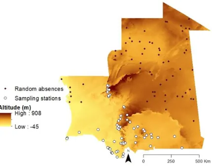
We built a generalized linear model (GLM) with a gaussian distribution in R and obtained a first global model for species richness. For this purpose, we generated random absences after applying a 200 km buffer around the sampling stations. We then fitted all possible simple models using the dredge function from the MuMIn v.1.15.6 (Barton, 2016) R package and ranked them following the Akaike information criterion with the correction for small sample sizes (AICc) and selected the model with lower AICc. We performed cross-validation to study model stability and predictive performance (Efron & Gong, 1983; Snee, 1977; Zhang, 1997). We randomly partitioned the dataset into a training subset consisting approximately of 4/5 of the samples, used to build the model following the same procedure as before and to estimate the coefficients; and a validation subset with the remaining samples, used to run the model built in the previous step and to evaluate its predictive ability. Each subset contained equal number of presences and absences. We replicated this process 10 times. Selection criteria like AICc and cross-validation techniques such as data splitting

(40)

approaches also help avoiding overfitting as they tend not to favour such models (Burnham & Anderson, 2004; Olden & Jackson, 2000). We then searched for influential observations and repeated the model building and model validation processes without those to obtain the final best fitted model for 61 sampling localities and 61 random absences (Figure 7). The chosen GLM was imported into ArcMap to predict amphibian richness distribution in the whole study area.

(41)

4. Results

4.1. Phylogenetic reconstruction

All genera were recovered as monophyletic clades. The 14 formally described taxa formed highly supported monophyletic clades in all trees (Figure 8 to Figure 10). COI produced conflicting topologies with both RAG1 and COI+RAG1 partitioned dataset, but all species clades in COI gene tree are confirmed by the two other reconstructions. All topologies divide most of the sequences in two major clades (Figure 8 to Figure 10). Contrary to the mitochondrial reconstruction, the combined COI+RAG1 and RAG1 topologies returned Leptopelis bufonides as sister clade of genus Kassina, and

Tomopterna and Pyxicephalus, from the family Pyxicephalidae, as a strongly supported

clade (Figure 8 to Figure 10).

The COI+RAG1 and mitochondrial marker split Hoplobatrachus occipitalis in two well supported clades (Figure 8 to Figure 10), confirmed by RAG1 but with lower support values (PP = 0.92 for both groups; Figure 9).

(42)

Figure 8. Phylogenetic reconstruction inferred from COI extended dataset I including sequences from GenBank (family

names in grey). Outgroup is not shown. Support values are provided as Bayesian posterior probabilities above branches (PP: * ≥ 0.99; ° 0.90 – 0.99).

(43)

Figure 9. Phylogenetic reconstruction inferred from RAG1 extended dataset II including sequences from GenBank

(family names in grey). Outgroup is not shown. Support values are provided as Bayesian posterior probabilities above branches (PP: * ≥ 0.99; ° 0.90 – 0.99).

(44)

Figure 10. Phylogenetic reconstruction inferred from COI and RAG extended datasets I including sequences from

GenBank (family names in grey). Outgroup is not shown. Support values are provided as Bayesian posterior probabilities above branches (PP: * ≥ 0.99; ° 0.90 – 0.99).