Decomposition Analysis of energy-related CO2 emissions in the USA and their decoupling from economic growth

UNIVERSIDADE DA BEIRA INTERIOR

Ciências Sociais e Humanas

Decomposition Analysis of energy-related CO2

emissions in the USA and their decoupling from

economic growth

João André Silva Pereira

Dissertação para obtenção do Grau de Mestre em

Economia

(2º ciclo de estudos)

Orientador: Prof. Doutor António Manuel Cardoso Marques

ii

Agradecimentos

Primeiramente, quero agradecer aos meus pais, Décio e Clara, por me proporcionarem a oportunidade de passar 5 anos fantásticos na Covilhã e por todo o apoio que me deram durante estes anos em que estive fora de casa, sem vocês nada disto seria possível.

Quero agradecer ao meu orientador, o Professor Doutor António Marques, pelo apoio e orientação dados durante a elaboração da minha dissertação.

A todas as amizades, que fiz ao longo destes 5 anos, por terem tornado esta cidade a minha 2ª casa, e por todos os momentos de alegria e descontração passados na vossa companhia. À minha namorada, Carolina, pelo apoio dado ao longo deste ano, por todas as vezes que me “obrigou” a trabalhar nesta dissertação que agora concluo, um muito obrigado, sem ti tudo teria sido mais difícil.

A todos vocês, obrigado por terem feito parte de todo este processo e por terem tornado estes últimos anos como estudante verdadeiramente inesquecíveis!

iii

Resumo

Os EUA, na última década, conseguiram reduzir as suas emissões de CO2 relacionadas com o consumo energético, sendo em 2016 14% mais baixas do que os níveis registados em 2005. Este trabalho visa identificar os drivers das alterações nas emissões de CO2 relacionadas com o uso energético e os fatores que forçam essas mudanças. Para quantificar o impacto desses fatores nas mudanças das emissões de CO2, é utilizado o modelo completo de decomposição. O estudo abrange toda a economia dos EUA, que é desagregada em quatro setores principais (Indústria, Transportes, Elétrico e Outros setores) para o período compreendido entre 1997-2016. Os resultados mostram que, de entre os 4 fatores que levaram a alterações nos níveis de emissões, o efeito da intensidade energética e o efeito do índice de carbonização foram os que mais contribuíram para mitigar as emissões de CO2. Neste trabalho é também examinado o índice de descolagem para testar se a redução nas emissões foi suficiente para dissociar o crescimento económico das emissões de CO2. O status de descolagem mais observado durante o período analisado foi o status de “descolagem fraco”. Estes resultados, combinados com as tendências nas emissões de CO2, mostram a importância que a mudança na fonte de energia, de combustíveis com alto teor carbónico, como é o caso do carvão e do petróleo, para o gás natural, ocorrida na última década foi um impulsionador para a economia americana começar a reduzir as suas emissões de CO2. Esta redução foi também alcançada através de melhorias na eficiência energética da economia.

Palavras-chave

iv

Resumo Alargado

A crescente preocupação com as mudanças climáticas levou este assunto ao debate político em todo o mundo. Nos EUA, ao longo dos anos, o assunto foi deixado para segundo plano, mas recentemente, em 2014, o presidente dos EUA fez uma declaração inédita, de que os EUA iriam reduzir as suas emissões de gases de efeito estufa (GEE) em 26% -28% abaixo dos níveis de 2005 até 2025. Esse compromisso foi posteriormente confirmado em 2015 durante a conferência COP21, realizada em Paris que reuniu líderes mundiais para debater eventuais medidas que visassem a redução das emissões de GEE mundiais. Esta conferência estabeleceu um marco histórico, pois foi a primeira vez que foi possível chegar a um acordo entre todos os participantes com o objetivo de manter o aquecimento global abaixo dos 2ºC até 2100. A participação dos EUA no acordo de Paris aumentou as esperanças da comunidade internacional em reduzir as emissões de GEE mundiais e atenuar as mudanças climáticas. Infelizmente, após a eleição de 2016, o governo eleito começou a revogar as políticas climáticas do governo anterior, retirando os EUA do acordo de Paris e revogando o Clean Power Plan, tornando a meta de redução das emissões até 2025 dificilmente alcançável.

Os EUA são hoje, o líder mundial em termos energéticos,pois, de acordo com o IEA 2017 World Energy Outlook, os EUA estão a caminho de se tornar energeticamente independentes, devido aos avanços tecnológicos que permitiram a exploração do gás de xisto . Em termos de petróleo e gás natural, os EUA superaram países como a Rússia e a Arábia Saudita. Segundo a BP Statistical Review of the World Energy 2018, os valores de 2017 da produção de gás natural aumentaram cerca de um terço quando comparados com a produção de gás natural de 2005, sendo 420,8 Mtep em 2005 e atingindo quase 632 Mtep em 2017. A produção de petróleo, de acordo com a BP Statistical Review of the World Energy 2018, foi de 309 Mt em 2005, mas esse valor aumentou quase 46% em 2017, com uma produção anual de 571 Mt de petróleo. Para entender este rápido aumento na produção de petróleo, é necessário dar algum contexto, BP Statistical Review define petróleo como “petróleo bruto, petróleo apertado, areias betuminosas e líquidos de gás natural”. A produção de petróleo apertado nos EUA sofreu um forte aumento desde 2010, atingindo o seu pico em 2015, com uma produção de 4,9 milhões de barris por dia, representando mais de 50% da produção de petróleo dos EUA (Energy Information Agency, 2017). Este aumento é o resultado do progresso técnico que fez com os custos de perfuração reduzissem e fez aumentar a eficiência da perfuração (Energy Information Agency, 2017). No caso da produção de gás de xisto, ao contrário do petróleo apertado, iniciou o seu boom em 2005 e desde então a produção aumentou cerca de 50% entre 2005 e 2015, atingindo 27 tcf, e, colocando assim, os EUA como o maior produtor mundial de gás natural.

Assim, sendo os EUA a maior potência energética mundial, torna-se importante estudar as suas emissões de CO2 relacionadas com o uso energético, para melhor entender o

v que provoca alterações nos níveis deste gás e assim fornecer aos decisores políticos mais uma ferramenta para auxiliar a elaboração de políticas que visem a redução das emissões de CO2 relacionadas com o uso energético.

Ao aplicar o método completo de decomposição (Sun, 1998), o presente trabalho visa identificar quais os fatores que provocam alterações nos níveis de emissões de CO2 e tornar-se assim, uma ferramenta para avaliar a eficácia das políticas adotadas pelas administrações dos EUA para mitigar as emissões de CO2 e as mudanças climáticas. No presente trabalho é também calculado o índice de descolagem para examinar se a economia americana conseguiu dissociar as emissões de CO2 do crescimento económico.

Os resultados mostraram que, em relação à análise da decomposição, todos os setores, á exceção do setor dos Transportes, incluídos neste trabalho conseguiram reduzir as suas emissões, dando assim o seu contributo para o progresso de descolagem. A intensidade energética foi fundamental para conseguir reduzir as emissões de CO2, tendo o seu contributo sido, claramente, superior aos contributos dos restantes efeitos. Através da análise à decomposição realizada para cada setor, o efeito da intensidade energética teve um impacto negativo nas emissões para quase todos os períodos analisados em cada setor. Isso implica que a intensidade energética dos EUA tem diminuído ao longo dos anos, refletindo as melhorias tecnológicas que foram desenvolvidas durante esses anos.

O índice de descolagem foi calculado com os resultados obtidos através da aplicação do método completo de decomposição. O status que apareceu com mais frequência foi o status de descolagem fraca, surgindo em 9 períodos. Este resultado significa que a economia dos EUA está a crescer mais rapidamente do que os seus níveis de emissões.

Novos estudos nesta área devem ser incentivados, principalmente para estudar o impacto que o gás de xisto está a ter na economia dos EUA, assim como estudar a alteração da composição dos GEE provocada pelo uso dessa fonte de energia, que ao contrário do carvão, é rica metano (CH4) e tem um baixo conteúdo carbónico.

vi

Abstract

The USA, for the past decade, have been able to reduce their CO2 emissions from energy-use being in 2016 14% lower than they were in 2005. This paper aims to identify the drivers behind the changes in energy related CO2 emissions and the factors that force those changes. To quantify the impact of these factors on the changes in CO2 emissions it is employed the complete decomposition model. This work covers the entire US economy, disaggregated in 4 major sectors (Industry, Transport, Electric and Other sectors) for the period 1997-2016. The results show that among the 4 factors that led to alterations on the emissions levels, the energy efficiency effect and the carbonization index effect were the major contributors to mitigate CO2 emissions. In this paper it is also examined the decoupling index to further understand if the reduction in the emissions was sufficient to decouple economic growth from CO2 emissions. The most common decoupling status observed during the analyzed period was the “Weak Decoupling” status. These results, combined with recent CO2 emissions trends show the importance that the shift in the energy sources from high carbon content fuels, like coal and petroleum, to natural gas that took place in the last decade gave a boost for the American economy to start reducing its CO2 emissions. This reduction was also achieved through improvements in energy efficiency in the economy.

Keywords

vii

Table of contents

1.Introduction ... 1

2.Literature Review ... 3

3.Data and method ... 5

3.1.Data ... 5

3.2.Data Analysis ... 5

3.2.1.Energy Related CO2 emissions ... 5

3.2.2.Primary Energy Consumption ... 6

3.2.3.Gross Output ... 7 3.3.Method... 9 4.Results ... 11 5.Discussion ... 19 6.Conclusion ... 23 7.References ... 24

viii

Figures List

Figure 1 – Energy related CO2 emissions Figure 2 – Primary Energy Consumption Figure 3 – Gross output

ix

Tables List

Table 1 – Variables Descriptive Statistics

Table 2 – Decomposition analysis of CO2 emissions from energy use from Other Services sector Table 3 – Decomposition analysis of CO2 emissions from energy use from Industry sector Table 4 - Decomposition analysis of CO2 emissions from energy use from Transport sector Table 5 - Decomposition analysis of CO2 emissions from energy use from Electric sector Table 6 - Decoupling Index and Status

x

Acronyms list

GHG Greenhouse Gas

SDA Structural Decomposition Analysis IDA Index Decomposition Analysis EU European Union

xi

1

1.Introduction

The increasing concern about the climate change has led this subject to the actual political debate worldwide. In the USA, over the years, the subject has been relegated to second plan, but recently, in 2014, the US administration made a never seen declaration that the US would reduce its greenhouse gas (GHG) emissions by 26%-28% below the 2005 levels by 2025. This commitment was further confirmed in 2015 during the COP21 conference, that was held in Paris and gathered leaders from all over the world to debate measures that could help reducing GHG’s emissions worldwide. This conference set an historical landmark, because it was the first time that it was possible to reach an agreement between all the participants with the objective of keeping global warming below 2ºC until 2100. The US participation on the Paris agreement rose the hopes of the international community in reducing the world GHG’s emissions and mitigate the climate changes. Unfortunately, after the 2016 US election, the elected administration started to revoke the previous administration climate agenda, pulling out the US of the Paris agreement and repealing the Clean Power Plan making the 2025 emissions target almost impossible to achieve.

The USA is today, the world’s undisputed energy leader, according to the IEA 2017 World Energy Outlook, the USA is on track to become energy independent, due to the shale revolution. In terms of oil and natural gas, the USA surpassed countries like the Russian Federation and Saudi Arabia. According to the 2018 BP Statistical Review of the World Energy, the values of the 2017 natural gas production increased about 1/3 when compared to the 2005 natural gas production, being 420,8 Mtoe in 2005 and reaching almost 632 Mtoe in 2017. The oil production, according to the BP Statistical Review of the World Energy 2018, was about 309 Mt in 2005 but in 2017 that value increased almost 46% with an annual production of 571 Mt of oil. To understand this rapid increase in oil production it is necessary to give some context, BP Statistical Review defines oil as “crude oil, tight oil, oil sands and natural gas liquids." Tight oil production in the USA suffered a sharp rise since 2010 peaking at 2015 with a production of 4.9 million barrels per day representing more than 50% of the USA oil production (Energy Information Agency, 2017). This increase is a result of technological improvements that have reduced the drilling costs and increased drilling efficiency (Energy Information Agency, 2017). In the case of shale gas production, unlike the tight oil, it started its boom in 2005 and since then the production increased around 50% between 2005 and 2015 reaching 27 trillion cubic feet and placing the USA as the world top natural gas producer.

With this work it’s expected to contribute to the literature on this subject regarding the USA by using a different approach. Also, with the identification of the effects that provoke changes on the energy-related CO2 emissions, this work can be used as tool to help defining new policies aiming to further reductions in CO2 emissions.

2 By applying the complete decomposition method (Sun, 1998), the present work aims to understand the factors that determine the alterations in CO2 emissions levels and to be a tool to evaluate the effectiveness of the policies that the US administrations took over the years to mitigate the CO2 emissions and the climate changes. It was also calculated the decoupling index to examine if the American economy performed decoupling between CO2 emissions and economic growth.

To apply the complete decomposition method the economy was divided in 4 sectors, the Industrial sector, the Electric sector, the Transport sector and the Other Services (including the residential and commercial sectors). The complete decomposition method was implemented through sectoral annual data (from 1997 to 2016) for the energy related CO2 emissions, the primary energy consumption and the gross output of each sector. Data from CO2 emissions and energy consumption were both collected from the US Energy Information Administration and data for the gross output was collected from the US Bureau of Economic Analysis.

With this work, I intend to identify the effects and the sectors that are contributing to increase energy-related CO2 emissions and those who are contributing to mitigate those alterations in the USA. It is also expected to identify the periods in which the American economy decoupled energy-related CO2 emissions from economic growth and the periods when it didn’t occur, and, to identify events that led the US economy to decouple, or not, CO2 emissions from economic growth.

This work is further presented as it follows: in the next section it will be presented the literature review. The third section is reserved both to the data used in the present paper and to the method applied. In the fourth section it will be presented the results obtained by applying the method that was presented in the previous section. The fifth is reserved to the discussion of the results. On the sixth and final section it will be presented the conclusion of this work.

3

2.Literature Review

Decomposition analysis was introduced in the late 70’s to fully comprehend the impact of structural change on industrial energy use. Nowadays this kind of analysis is widely used to understand the drivers behind CO2 emissions.

There are two main decomposition methods, the structural decomposition analysis (SDA) and the index decomposition analysis (IDA). A full comparison between these two methods was made by Hoekstra & van der Bergh (2003). They concluded that SDA is capable of more refined decompositions of economic and technological effects because it uses the input-output model while the IDA uses more aggregated sector data resulting in more detailed time and country studies because of the availability of data. Xu and Ang (2013) concluded that IDA method is recognized by researchers as a useful analytical tool to understand CO2 emissions drivers.

There are two main approaches for the IDA method, the Laspeyres and the Divisia method. The Laspeyres method is based on the Laspeyres index and was first introduced by Howarth et al (1991). The Laspeyres method has a big disadvantage because it led to a large residual term leading to an also large estimation error. In 1998, Sun (1998) introduced a complete decomposition method based on the Laspeyres method that solved the residual term problem associated with the Laspeyres method by distributing the residual terms trough the considered effects. The Divisia method is used through the arithmetic mean Divisia index (AMDI) and the logarithmic mean Divisia index (LMDI) and its properties were examined and discussed by Xu & Ang (2013).

There have been published a few papers trying to identify the emissions drivers on a sectoral level, like industry, including manufacturing, and agriculture. Liaskas et al (2000) studied the industrial CO2 emissions of 13 EU countries and concluded that despite the continuous growth of the industrial production, CO2 emissions have been decreasing in the manufacturing sector, except for less developed EU countries, as Portugal and Greece. Diakoulaki & Mandaraka (2007) performed a study to assess the progress in decoupling the industrial emissions in the manufacturing sector of 14 EU countries. By applying the complete decomposition method, they found that only 7 out of 14 countries managed to separate CO2 emissions from industrial growth. Robaina-Alves & Moutinho (2014) used the complete decomposition method to study GHG emissions for the agriculture sector for a set of European countries showing that in the 1995-2008 period there was an increase on the sector emissions. Roinioti & Koroneos (2017) applied the complete decomposition method to study Greeces decoupling progress before and during the economic crisis. They concluded that the energy intensity was the main contributor to the CO2 emissions decrease during the analyzed period. They also found that during the economic crisis, the decoupling status was not achieved, concluding that the economic crisis interrupted the decoupling progress that was attained before the crisis.

4 The decomposition analysis has also been applied to non-EU countries, being China the most studied country. Paul & Bhattacharya (2004) used the complete decomposition method to study the drivers behind energy-related emissions in India. Freitas & Kaneko (2011) used a decomposition method based on the LMDI method to decompose Brazil’s CO2 emissions. They found that the carbon intensity and the energy mix were the main contributors for the emission reduction observed in Brazil in the 2004-2009 period. Kumbaroğlu (2011) performed the complete decomposition method to study Turkish sectoral emissions.

The US have also been subjected to several studies to explore the emissions from different sources. Baldwin & Wing, (2013) employed LMDI method to study the evolution of CO2 emissions in the US. They found that the growth of both GDP pc and population were the main contributors of CO2 emissions overlapping the mitigating effects of a lower energy intensity and a changed composition of the output. Shahiduzzaman & Layton (2015) applied the LMDI method to explore emissions over business cycles and they concluded that both the aggregated emissions and the emissions intensity reduce much faster during contractions than they increase during economic expansions. Also, Shahiduzzaman & Layton (2017), employed the LMDI method to US sectorial emissions, to evaluate the possibility that the US have, to achieve their 2025 emissions target. They concluded that improvements in energy efficiency, declines in carbon intensity of energy as well as structural changes in the economy all had a major role in decreasing the emissions from 2001 to 2014. They also made projections for the emissions trends and concluded that without new policies that mitigate CO2 emissions, the US 2025 emissions target will be almost impossible to achieve. Jiang & Li (2017) applied both AMDI and LMDI methods to explore the emissions from electric output and their decoupling from economic growth. They found that both the energy conversion efficiency and the fuel-mix effect were the main contributors for curbing the emissions. They also observed that the “No Decoupling” was the most observed status during the analyzed period.

5

3.Data and method

3.1.Data

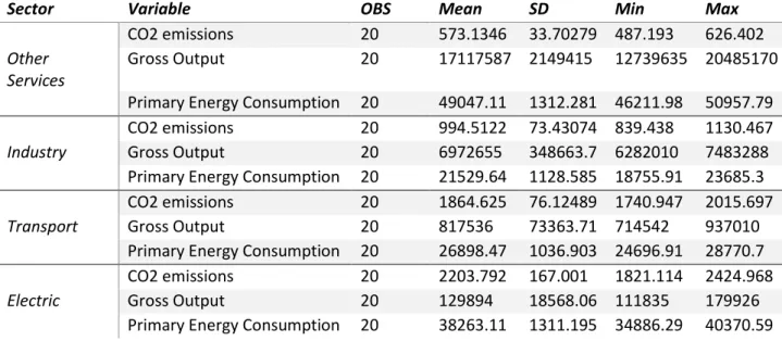
In this paper the American economy will be divided in four sectors: Industrial, Transportation, Electric and Other services (including residential and commercial sectors) (Shahiduzzaman & Layton, 2017). To conduct this analysis, it will be used three variables (Roinioti & Koroneos, 2017): CO_2 emissions from energy consumption (Million metric tons), energy consumption (Million BTU) and Gross-Output (Millions of chained (2009) dollars) of each sector. The gross-output data was chosen over value added data because of the availability of disaggregated data regarding the electric sector. The data for CO2 emissions and energy consumption were collected from the US Energy Information Agency and data for gross output was collected from Bureau of Economic Analysis from 1997 to 2016.

In table 1 it is presented the descriptive statistics for the sectoral data used in this work.

Table 1- Variables Descriptive Statistics

Sector

Variable

OBS

Mean

SD

Min

Max

CO2 emissions

20

573.1346

33.70279 487.193

626.402

Other

Services

Gross Output

20

17117587 2149415

12739635 20485170

Primary Energy Consumption 20

49047.11

1312.281 46211.98

50957.79

CO2 emissions

20

994.5122

73.43074 839.438

1130.467

Industry

Gross Output

20

6972655

348663.7 6282010

7483288

Primary Energy Consumption 20

21529.64

1128.585 18755.91

23685.3

CO2 emissions

20

1864.625

76.12489 1740.947

2015.697

Transport

Gross Output

20

817536

73363.71 714542

937010

Primary Energy Consumption 20

26898.47

1036.903 24696.91

28770.7

CO2 emissions

20

2203.792

167.001

1821.114

2424.968

Electric

Gross Output

20

129894

18568.06 111835

179926

Primary Energy Consumption 20

38263.11

1311.195 34886.29

40370.59

3.2.Data Analysis

3.2.1.Energy Related CO2 emissions

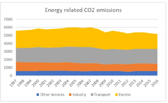
CO2 emissions are strongly related with energy consumption and it is important to understand the recent energy-related CO2 emission trends. From 1997 to 2007 CO2 emissions increased about 7.3% and it can be attributed to the wealthy US economy, that was in expansion during those years. It is possible to observe a drop on the emissions levels in 2007 that is consistent with the economic recession that started in the USA and then propagated to the rest of the world. The economic crisis slowed down the US economy and restrained the US

6 economic activity. As consequence of the restrained economy, between 2008 and 2011 the USA dominated the global CO2 emissions reduction (Xuemei Jiang & Guan, 2017).

Figure 1-Energy-related CO2 emissions

Source: EIA 2017

During the analyzed period the sector who most reduced its energy related emissions was the Industry sector with a reduction of about 20% between 1997 and 2016. This reduction can be attributed to the substitution of the energy sources used in industry, to the improvements in energy efficiency, to the financial crisis and to the separation of the production and consumption. For example, the manufacturing industries managed to reduce by half their emissions on US soil by half between 1992 and 2009, but in that same timespan the imports from low wage countries increased from 7% to 23% (Li & Zhou, 2017). Overall, the USA managed to reduce its energy-related CO2 emissions, the Electric sector reduced its emissions by 15% and the Other Services had a reduction of about 12%, but the Transport sector was the only sector, within the ones presented in this study, that increased its emissions during the analyzed period (Highway Statistics, 2016).

3.2.2.Primary Energy Consumption

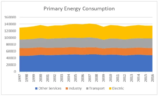
The US primary energy consumption have been increasing since 1997. From 1997 to 2016, the timespan used in this work, the primary energy consumption increased about 4%. Before the crisis, the US energy consumption rose from 129480,5 to 141386 trillion BTU (Monthly Energy Review, June 2017) between 1997 and 2007, representing an increase of about 8%. Along with the CO2 emissions presented on figure 1, this increase is a result of the wealthy American economy that was flourishing during those years. During that timespan the only sector who decreased its energy consumption was the Industry sector with a reduction of

7 almost 11%. It is important to say that during this period the Industry sector also reduced its economic share in the US economy. The sector who most increased its energy consumption was the transport sector followed by the energy sector. The increase in the energy consumption of the transport sector is due to increase of motor vehicles that increased about 16% during that period (Highway Statistics, 2016).

Figure 2-Primary energy consumption

Source : EIA 2017

The energy consumption peaked in 2007 and suffered a drop in 2008 but since then it remained somehow steady suffering slight oscillations. Between 2007 and 2016 the sector who most reduced its consumption was the Electric sector followed by the Other Services sector. The electric sector decrease in the energy consumption can be attributed to the stagnation of electricity sales to ultimate consumers (Electric Power Monthly, May 2018) and the switch from coal to natural gas that is a more efficient energy source. In the overall, apart from the Industry sector, all the sectors increased their primary energy consumption being the transport sector the one that registered the biggest increase of about 11%.

3.2.3.Gross Output

The gross output data, as it was explained previously on this work, will be used as a proxy of the economic growth. As it can be observed through the analysis of figure 3, the US gross output have been increasing during the timespan chosen for this work. From 1997 to 2016 the US gross output increased 30%, clearly showing that the economy was in expansion. Nevertheless, during the financial crisis years (2007-2009), it is possible to observe a drop in the gross output of about 8%.

8

Figure 3- Gross Output

Source: Bureau of Economic Analysis 2017

The Other Services sector, during the studied timespan, increased its gross output in about 38%. It was the biggest increase from all of the 4 sectors included in this study. The Industry sector increased its gross output in about 12%, the Transport sector in 23% and the Electric sector in about 9%. In the overall, as it was expected by analyzing figure 3, all the 4 sectors presented in this study increased its gross output. From the comparison of the values for the Other Services sector and the Industry sector, it’s possible to conclude that the US economy is in a transition to a less industrialized and more service-oriented country.

9

3.3.Method

To perform this analysis, it will be implement the decomposition method proposed by Sun (1998) to achieve a better understanding of emissions drivers. The decomposition method proposed by Sun is one of the techniques of the IDA family and its based on the modified Laspeyres index. Kaya Identity it will be used to express the effects that causes alterations on the emissions levels.

Sun (1998) decomposition method will be used to decompose emissions of the sectors (i) in the period (t), being estimated as the product of the carbon intensity (CIit_), energy intensity (EIit), the economic share of the sector (Sit) and the economic activity (Git). The emissions can be expressed by Kaya Identity as it is show in the following equations:

( 1)

, ( 2)

where n represents the number of economic sectors, the emissions of the sector i in the period t, the energy consumption of the sector i in the period t, the value added of the sector i in the period t and the value added of the US economy in the period t. The variation of the emissions in each period can be expressed as the difference of the emissions on that two periods.

( 3)

( 4)

Where,

: stands for the carbonization index effect : stands for the energy intensity effect : stands for the structural effect : stands for the economic activity effect

The effects can be calculated by the following equations:

( 5)

10 ( 7)

( 8)

The sum of the 4 effects described above or the difference between the total variation of emissions and the economic activity effect gives us the curbing effect on emissions

( 9) The decoupling index gives us the detachment level between emissions and economic growth. In this work, it will be used the decoupling index presented by Diakoulaki & Mandaraka, 2007. If , the decoupling index can be calculated by:

( 10)

where, stands for the decoupling index, , and represents the impact of the carbon intensity, energy intensity and structural effect on the decoupling development correspondingly. If the economic activity effect turns out to be negative, we can say that economic growth had a negative impact on emissions and contributed to curb the emissions. Therefore, the curbing effect on should be analysed without the economic activity effect. Then, if , the decoupling index can be calculated by the following equation:

( 11)

If , there was a strong decoupling between the emissions and economic growth, if , there was a weak decoupling between the emissions and economic growth, and, if ,we can say that there was no decoupling between the emissions and economic growth.

11

4.Results

The results presented in this section were obtained through the application of the complete decomposition method also known as the refined Laspeyres index. This method was presented by Sun (1998) to solve the Laspeyres decomposition method (Howarth et al, 1991 and Park, 1992) main problem. The problem about the Laspeyres decomposition method was that it led to a large residual term that posed an obstacle to the interpretation of the results obtained through the implementation of the method. To solve this problem, Sun (1998) applied the “jointly created, equally distributed” principle to distribute the residual term by the main effects dissipating its effect and achieving more robust results. According to Ang & Zhang (2000) the refined Laspeyres method passes the test for time-reversal, factor-reversal and zero-value robustness test.

As it was explained in the previous section, to obtain these results, it was used three variables, CO2 emissions from energy consumption (Million metric tons), energy consumption (Million BTU) and gross-output (Millions of chained (2009) dollars) for each sector. The main issue with the data used in this paper is the use of the gross output instead of sectoral value-added data, because it can double count intermediate consumption. But, as it was explained previously in this work, the unavailability of value-added data regarding the electric sector, led us to use gross output data as weaker proxy of the sectoral economic growth. With the results obtained through the complete decomposition method, it is calculated the decoupling index. The decoupling index calculated in this paper was introduced by Diakoulaki and Mandaraka (2007) because it expurgates the effect of the economic activity from the decoupling effect when the economic activity effect is negative, because it is implied that if the effect is negative it will contribute to mitigate CO2 emissions therefore the decoupling index should be examined after the removal of this effect.

Over this section, it will be presented a table with the results obtained after the application of the complete decomposition method for each of the sectors presented in this paper, the Other Services, the Industry, the Transport and the Electric sector, and in the end it will be presented a table with the decoupling index and status for each period that is comprised in the timespan of this work, 1997 to 2016.

Table 2 shows us the results obtained for the Other Services sector. This sector is comprised of all the sectors of the US economy that are not included in the other sectors presented in this paper, and by that, it is the vastest and more diversified sector included in this paper. By analyzing the table presented below, the economic activity is the major promoter of this sector emissions, contributing to its increase in all of the periods analysed in this paper, with the exception of the financial crisis years, 2007-2008 and 2008-2009 clearly showing the impact that economic activity has in CO2 emissions.

12 This sector has been increasing its proportion in the US economy as can be shown by the Sectoral effect values, indicating a shift in the economy to a more service-oriented economy. Sectoral effect only contributed to reduce CO2 emissions in the post financial crisis. Both the energy intensity effect and the carbonization index effect, overall, played a mitigating role in CO2 emissions.

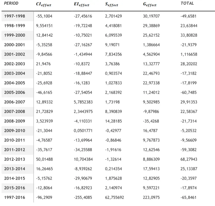
Table 2- Decomposition analysis of CO2 emissions from energy use from Other Services sector (1000 metric tons of CO2)

PERIOD TOTAL 1997-1998 -55,1004 -27,45616 2,701429 30,19707 -49,6581 1998-1999 9,554151 -19,72248 4,418081 29,38869 23,63844 1999-2000 12,84142 -10,75021 6,095539 25,62152 33,80828 2000-2001 -5,35258 -27,16267 9,19071 1,386664 -21,9379 2001-2002 -9,84566 -1,434944 7,834356 4,562904 1,116658 2002-2003 21,9476 -10,8372 3,76386 13,32777 28,20202 2003-2004 -21,8052 -18,88447 0,903574 22,46793 -17,3182 2004-2005 -25,6928 -16,1283 1,027833 22,97338 -17,8199 2005-2006 -46,6165 -27,54054 2,168392 11,24012 -60,7485 2006-2007 12,89332 5,7852383 1,73198 9,502985 29,91353 2007-2008 21,72829 2,3443975 8,390839 -9,87986 22,58367 2008-2009 3,523939 -4,110331 14,28185 -35,4268 -21,7314 2009-2010 -21,3044 0,0501771 -0,42977 16,4787 -5,20532 2010-2011 -4,76587 -13,69964 -0,86846 9,767873 -9,56609 2011-2012 -35,7617 -34,25588 -1,91616 12,62546 -59,3082 2012-2013 50,01488 10,704384 -1,32614 8,886309 68,27943 2013-2014 16,26465 -8,939262 0,214354 17,59413 25,13387 2014-2015 -5,15762 -29,90679 1,875628 12,82905 -20,3597 2015-2016 -12,8064 -16,82923 2,140974 9,597221 -17,8974 1997-2016 -96,2909 -255,4085 62,755692 223,0975 -65,8461

The carbonization index presented a negative sign on the majority of the analyzed period. Nevertheless, during the financial crisis years, 2006 to 2009, the carbonization index turns to be positive, or in, other words, it contributed to increase CO2 emissions. This indicates that while the economy was in contraction this sectors carbon intensity worsened. But, as it was written before, the overall effect of the carbon index was clearly to reduce CO2 emissions. This clearly indicates a shift towards more efficient and cleaner energies like

13 natural gas. The biggest contributor for reducing CO2 emissions was clearly the energy intensity effect, that was negative (contributed to reduce CO2 emissions) for almost every period during the selected timespan. This result was achieved through improvements in energy efficiency that led to a drop in energy intensity. This decrease in the USA energy intensity can be explained with the energy efficiency programs and policies (Appliance standards, Building codes …) and warmer winter weather as the most important contributors for the decline in energy consumption in the residential and commercial sectors (Nadel & Young, 2014).

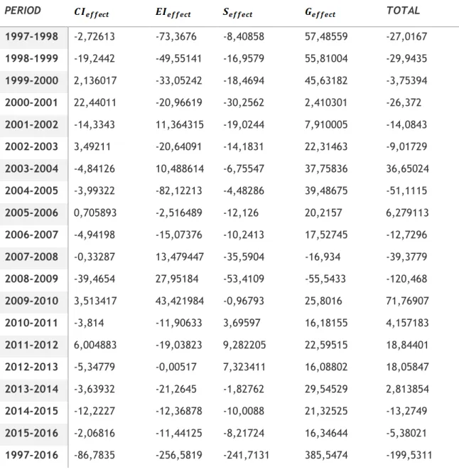
Table 3 shows us the decomposition analysis performed to the Industry sector. This sector is the 2nd largest presented in this work, as it can be observed by the value of the mean gross output, presented on table 1. This sector, throughout the years, has been able to reduce its CO2 energy related emissions. From a quick analysis performed to table 3, from the 4 effects selected to explain the changes behind CO2 emission levels, the energy intensity effect followed by the sectoral effect were the ones who most contributed to the mitigating progress. The carbon intensity effect also contributed to this decrease, but in a lesser extent than the previous effects. The economic activity effect was the only that appeared positive when analyzing the 1997-2016 period.

As it can be observed through the analysis of the table 3, this sector did well in reducing its energy-related CO2 emissions. As it was already written during the analysis of Figure 1, the Industry sector, between the sectors included in this work, was the one who recorded the biggest drop in CO2 emissions. Table 2 shows us that on this sector, both the carbon intensity effect, the energy intensity effect and the structural effect had a mitigating role in CO2 emissions. These 3 effects were presented with a negative sign in the majority of the analyzed periods. Through the analysis of the sectoral effect it is possible to identify a retraction of this sector in the US economy. The carbon intensity effect indicates that the Industry sector is shifting towards cleaner fuels. The energy intensity effect shows the improvements that the sector had in terms of energy efficiency, with new technologies being developed to reduce CO2 emissions and to consume less energy. The economic activity effect was positive during the analyzed period, except for the financial crisis years, indicating a strong relationship between the economic activity and CO2 emissions. This relationship was already observed during the analysis of the decomposition analysis performed for the Other Services sector. The Industry sector drop in emissions levels can also be explained through the separation of the production and consumption of goods. Li & Zhou (2017) found that US industries reduced their pollution levels by offshoring their production to low wage and less regulated countries, but this problem will be addressed later in this paper. Through the analysis of the decomposition analysis performed to the Industry sector, it is possible to observe that this sector was successful to reduce its CO2 emissions on the US soil.

14

Table 3-Decomposition analysis of CO2 emissions from energy use from Industry sector (1000 metric tons of CO2) PERIOD TOTAL 1997-1998 -2,72613 -73,3676 -8,40858 57,48559 -27,0167 1998-1999 -19,2442 -49,55141 -16,9579 55,81004 -29,9435 1999-2000 2,136017 -33,05242 -18,4694 45,63182 -3,75394 2000-2001 22,44011 -20,96619 -30,2562 2,410301 -26,372 2001-2002 -14,3343 11,364315 -19,0244 7,910005 -14,0843 2002-2003 3,49211 -20,64091 -14,1831 22,31463 -9,01729 2003-2004 -4,84126 10,488614 -6,75547 37,75836 36,65024 2004-2005 -3,99322 -82,12213 -4,48286 39,48675 -51,1115 2005-2006 0,705893 -2,516489 -12,126 20,2157 6,279113 2006-2007 -4,94198 -15,07376 -10,2413 17,52745 -12,7296 2007-2008 -0,33287 13,479447 -35,5904 -16,934 -39,3779 2008-2009 -39,4654 27,95184 -53,4109 -55,5433 -120,468 2009-2010 3,513417 43,421984 -0,96793 25,8016 71,76907 2010-2011 -3,814 -11,90633 3,69597 16,18155 4,157183 2011-2012 6,004883 -19,03823 9,282205 22,59515 18,84401 2012-2013 -5,34779 -0,00517 7,323411 16,08802 18,05847 2013-2014 -3,63932 -21,2645 -1,82762 29,54529 2,813854 2014-2015 -12,2227 -12,36878 -10,0088 21,32525 -13,2749 2015-2016 -2,06816 -11,44125 -8,21724 16,34644 -5,38021 1997-2016 -86,7835 -256,5819 -241,7131 385,5474 -199,5311

Table 4 shows us the decomposition analysis performed to the Transport sector. This sector is responsible for most of the energy-related CO2 emissions in the USA, accounting for about 36 % of the total CO2 emissions (Monthly Energy Review, June 2017). Transport sector was the only sector that increased its emissions during the analyzed timespan, due to the impact of the economic activity effect that nullified the contribution of the other three sectors to the mitigating progress.

15

Table 4- Decomposition analysis of CO2 emissions from energy use from Transport sector (1000 metric tons of CO2) PERIOD TOTAL 1997-1998 1,859579 -32,87204 -21,8147 90,52594 37,6988 1998-1999 -2,50028 4,094957 -47,9912 92,35529 45,95873 1999-2000 1,759397 40,120223 -76,2234 78,63183 44,28804 2000-2001 -1,27848 75,137599 -98,8423 4,239039 -20,7441 2001-2002 0,789424 54,771336 -29,1424 14,26371 40,68206 2002-2003 -4,15234 -49,18173 10,94462 41,11381 -1,27565 2003-2004 0,223107 -68,52236 64,68043 69,83964 66,22081 2004-2005 -3,74534 -45,90599 1,22035 75,27805 26,84706 2005-2006 -2,38961 -59,6588 50,4699 39,97232 28,39382 2006-2007 -2,64763 -49,59037 23,84799 35,07238 6,682369 2007-2008 -27,5943 -51,86729 -9,42099 -33,7708 -122,653 2008-2009 -11,0041 160,63122 -100,403 -115,257 -66,0326 2009-2010 -8,23205 -64,02925 35,4331 54,14738 17,31918 2010-2011 -7,62406 -89,23494 33,22662 32,40905 -31,2233 2011-2012 -3,69305 -75,93557 -1,11147 43,85805 -36,882 2012-2013 -9,13519 8,472916 -3,24433 30,52142 26,61481 2013-2014 1,420411 -67,03361 27,50707 56,13467 18,02855 2014-2015 -0,66208 -15,71112 -1,05816 41,20835 23,77699 2015-2016 -9,21764 47,508984 -41,3673 32,36161 29,28565 1997-2016 -85,2791 -267,9347 -189,1753 673,034994 130,6458

During the analyzed period, the Transport sector was the one who most increased its emissions, since 1997, energy-related CO2 emissions from the Transport sector increased about 7%.This increase on emissions levels can be attributed to the increasing number of vehicles in circulation year after year that causes a rise in CO2 emissions levels as can be seen by economic activity effect that only had a negative impact on the recent crisis years. The energy intensity effect assumed the leading role in the sectors mitigating progress showing the improvements done in terms of public transportation and car engines that are now more efficient allowing to travel longer distances with less fuel. The other two effects, the carbon intensity effect and the structural effect, also contributed to decreasing the energy-related emissions from 1997 to 2016, indicating a shift to cleaner fuels, as biofuels that, according to the 2017 Transportation Statistics Annual Report, increased over 900 %

16 from 2000 to 2016 due to the requirements of the Federal Renewable Fuels Standard (RFS) that requires the introduction of increasing amounts of renewable energy in the common fuels used in transportation, as gasoline and diesel, year after year. Also, according to the same report the number of Electric Hybrid Vehicles(EHV) sales have been increasing since 1999 and peaked in 2013, suffering a slightly drop in the number of sold EHV since then. Unfortunately, the contribution of these effects was not enough to counterbalance the positive impact of the economic activity effect.

The Electric sector decomposition analysis is presented on table 5. This sector has been one the most contributors to energy-related CO2 emissions during the past 40 years. We can observe that, unlike as in the previous tables, the energy intensity effect wasn’t the main contributor to the sector emissions decrease. Nevertheless, the results show that there were improvements in the energy efficiency, indicating that the sector used the input energy more efficiently during the years. The carbon intensity effect played a negative role in the emissions levels, and this result was achieved through a shift to cleaner fuels to produce energy, like natural gas instead of petroleum or coal as the main energy source. The economic activity effect played a positive role in the emissions level for almost the entire period took under the analysis, except for the last economic recession years. With the reduction of CHP plants, the structural effect was the main contributor to the mitigating progress. Also, the shutdown of coal fired power plants will make room for more energy efficiency improvements in the sector that will result in lower energy intensity levels. The Electric sector is responsible for about 35% of the total energy-related CO2 emissions in the USA (Monthly Energy Review, June 2017). This sector has been able to decrease its emissions due to the shift in the energy source, from coal to natural gas. This substitution can be observed by analysing the decomposition analysis for the 1997-2016 period in which the carbon intensity effect had a major contribution to the mitigating progress. The sectoral effect was led the emissions decrease in this sector. This can be attributed to the decrease of Combined Heat and Power (CHP) Plants, that counted with about 274 plants in 2006 and in 2016 there were 234 CHP plants in the USA (Electric Power Annual,2016).

17

Table 5-Decomposition analysis of CO2 emissions from energy use from Electric sector (1000 metric tons of CO2) Period Total 1997-1998 9,564959 3,6954393 -33,2697 110,4034 90,39408 1998-1999 -32,566 -364,5411 296,6233 113,2818 12,79795 1999-2000 40,44187 -86,17946 55,42018 96,06269 105,7453 2000-2001 14,03936 -202,2742 145,4891 5,228346 -37,5174 2001-2002 -34,3337 1088,399 -1056,69 17,9568 15,32849 2002-2003 30,43848 81,621994 -131,074 50,19883 31,18568 2003-2004 -9,79448 41,813935 -85,7741 84,89798 31,14336 2004-2005 8,96987 -71,95754 37,02112 91,18195 65,21539 2005-2006 -44,6306 -50,97641 -9,46921 47,82586 -57,2504 2006-2007 9,42372 -144,8733 160,3563 41,69677 66,60344 2007-2008 -28,1033 -25,56191 43,0651 -41,4737 -52,0738 2008-2009 -104,75 90,879456 -60,9255 -140,088 -214,885 2009-2010 24,08154 -73,27674 96,32568 65,27459 112,4051 2010-2011 -82,3686 175,02054 -232,638 39,29242 -100,694 2011-2012 -72,329 -142,3862 27,97405 51,3934 -135,348 2012-2013 3,488064 49,839451 -72,636 34,8379 15,52939 2013-2014 -14,5294 76,337042 -125,333 63,51435 -0,01099 2014-2015 -99,2551 -276,0358 193,3195 44,8083 -137,163 2015-2016 -86,2989 -123,8261 86,14137 32,56126 -91,4223 1997-2016 -444,7755 -47,40409 -530,18979 712,8743 -309,49509

18

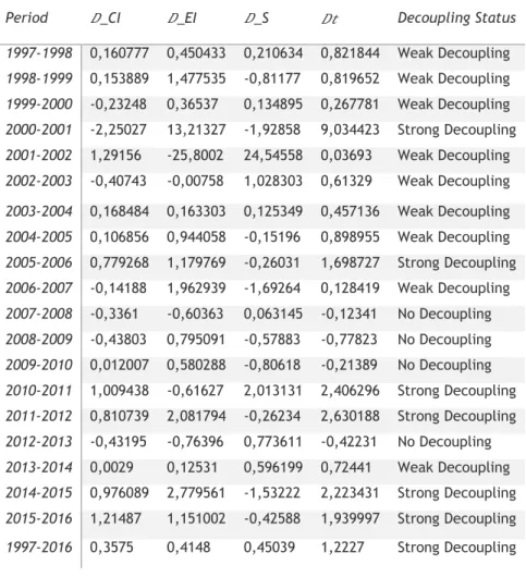
Table 6-Decoupling Index and Status

Table 6 shows us the decoupling between emissions and economic growth. We can observe that the most common status is Weak Decoupling, making 9 appearances during the analysed period, followed by the Strong Decoupling and the No Decoupling status with 6 and 4 observations correspondingly. The Weak Decoupling status means that, as the economy grows, CO2 emissions grows as well, but in a smaller proportion. This means that as the economy thrives, CO2 emissions also increase its levels due to the increase in economic activity. This status is commonly observed worldwide, because it is a consequence of the economic growth achieved worldwide. Also, the No Decoupling status registered during this analysis occurred when the economy was in recession. These results indicate that when the economy is weaker, it is harsher to dissociate emissions levels from the economic growth. It is possible to observe that between the chosen effects, the Energy Intensity effect and the Carbon Intensity effect were the ones who played a bigger contribution to the decoupling progress. The structural effect, overall, did not contributed to the decoupling progress.

Period _CI _EI _S Decoupling Status 1997-1998 0,160777 0,450433 0,210634 0,821844 Weak Decoupling 1998-1999 0,153889 1,477535 -0,81177 0,819652 Weak Decoupling 1999-2000 -0,23248 0,36537 0,134895 0,267781 Weak Decoupling 2000-2001 -2,25027 13,21327 -1,92858 9,034423 Strong Decoupling 2001-2002 1,29156 -25,8002 24,54558 0,03693 Weak Decoupling 2002-2003 -0,40743 -0,00758 1,028303 0,61329 Weak Decoupling 2003-2004 0,168484 0,163303 0,125349 0,457136 Weak Decoupling 2004-2005 0,106856 0,944058 -0,15196 0,898955 Weak Decoupling 2005-2006 0,779268 1,179769 -0,26031 1,698727 Strong Decoupling 2006-2007 -0,14188 1,962939 -1,69264 0,128419 Weak Decoupling 2007-2008 -0,3361 -0,60363 0,063145 -0,12341 No Decoupling 2008-2009 -0,43803 0,795091 -0,57883 -0,77823 No Decoupling 2009-2010 0,012007 0,580288 -0,80618 -0,21389 No Decoupling 2010-2011 1,009438 -0,61627 2,013131 2,406296 Strong Decoupling 2011-2012 0,810739 2,081794 -0,26234 2,630188 Strong Decoupling 2012-2013 -0,43195 -0,76396 0,773611 -0,42231 No Decoupling 2013-2014 0,0029 0,12531 0,596199 0,72441 Weak Decoupling 2014-2015 0,976089 2,779561 -1,53222 2,223431 Strong Decoupling 2015-2016 1,21487 1,151002 -0,42588 1,939997 Strong Decoupling 1997-2016 0,3575 0,4148 0,45039 1,2227 Strong Decoupling

19

5.Discussion

In this work it is applied the complete decomposition technique to explore, between the effects that cause alterations in CO2 emissions levels in the USA, the carbon intensity effect, the energy intensity effect, the structural effect and the economic activity effect, which contributed to curb CO2 emissions and the ones who promoted the emissions. Also, it is calculated a decoupling index to check the dissociation level between the economic growth and CO2 emissions. The most common decoupling status observed was the “Weak Decoupling” status, meaning that the emissions are growing at a slower pace than the American economy, which is represented by a proxy, the gross-output. This proxy has its own limitations in terms of measuring sectoral economic growth. It would be more suitable to use the industry value-added, but data regarding the electric sector value added was unavailable, and only for that reason the gross output was chosen to be a proxy of the sectoral economic growth.

The results showed that, concerning to the decomposition analysis, all the sectors, apart from the Transport sector, included in this work were able to reduce its emissions, and by that contributed to the decoupling progress. The energy intensity effect played the major role in decreasing CO2 emissions. Through the decomposition analysis performed to each sector and exposed in the previous section, the energy intensity effect had a negative impact on emissions for almost of the analyzed periods in each sector. This implicates that the energy intensity of the USA has been decreasing through the years reflecting the technological improvements that have been developed during these years. Metcalf (2008) in his analysis showed that the reduction in US energy intensity, at a state level, is mainly caused by improvements in energy efficiency as opposed to a shift from energy intensive activities to less energy intensive activities. Also, according to Nadel & Young (2014) ,the weather influenced the reduction in energy consumption , primarily on the Residential and Commercial sectors due to warmer winters that led to lower usage of temperature control devices.

The carbon intensity effect, overall, as the energy efficiency effect, contributed to reduce the emissions, indicating a shift towards cleaner energy sources. Since 2009, with the shale gas boom, natural gas passed coal to become the US leading energy source. The impact that these change in the energy production mix had on CO2 emissions was announced on the EIA Monthly Energy Outlook (October, 2016) that the US had registered the lowest CO2 energy related emissions in the first six months since 1991. Of course, the growth of renewable energies had their role in that reduction, but let’s not forget that RES only accounted for less than 11% of the US total energy consumption in 2016, and we can attribute the fall of coal consumption, caused by the substitution for natural gas, has the booster for that drop.

The other two effects, with a bigger extent to economic activity effect, contributed to increase CO2 emissions in the USA. It was no surprise that the economic activity effect

20 boosted the emission, because of the relationship between these two variables. If the economic activity is in expansion, so does the economy and so does the emissions.

The economic activity effect turned out to be negative only in two periods, 2007-2008 and 2008-2009, in all the economic sectors included in this study. These two periods were characterized by the economic recession that started in the US and propagated to the rest of the world. These results clearly show the link between these variables. Regarding the sectoral effect, it reflects the sectors position in the economy. It was possible to identify the shift in the US economy from an Industrialized economy to a service-oriented economy. From the analysis of the sectoral effect presented for all the sectors presented in this study, we can observe that the effect promoted CO2 emissions in the Other Services sector but contributed to reduce the emissions on the Industry sector. Also, the Industry sector was the only were the sectoral effect was predominantly negative showing the decline of the US industry. The Transport sector, as it has been said on the previous section, was the only one that during the analyzed timespan increased its CO2 energy related emissions. This was a result of the increasing number of vehicles in circulation in the USA, according to data presented on Highway Statistics 2016. The number of cars registered increased about 20% from 1997 to 2016. That is a consequence of the economic growth that the US suffered during most of the timespan, and it can be observed by looking at the values of the economic activity effect presented on table 4. We can see that only in 2007-2008 and 2008-2009, the economic activity effect turned to have a negative impact on CO2 emissions. Also, cheap fuel has contributed to increase that CO2 emissions levels. For instance, the average US car about emits about 251 gCO2/km as for instance, the average EU car emits 118 gCO2/km, but it is important to refer that in EU car fuel is heavily taxed and that reflects on the price. To compare, a liter of gasoline in the EU 28 costs on average 1,59 USD per liter and in the USA costs on average 0,83 USD per liter. Also, as the USA is a very large country, almost the same size as the European continent so cars drive longer distances than they do in EU, for instance an EU car drives an average of 12 009 km per year as an USA car drives an average of 21 688 km per year. All of this combined make the pollution of light duty vehicles very significant in the USA, and in 2016, light duty vehicles accounted for 60% of the sector total emissions. Also, the number of domestic flights has been increasing in the USA, and aviation accounted for 9% of the sector total emissions in 2016.

The Electric sector was the leading sector in terms of energy related CO2 emissions, but it has been successful to reduce its emissions, and has been surpassed by the transport sector in the last years. From the analysis of table 5, we can observe that both the carbonization intensity effect, the energy intensity effect and the structural effect contributed to curb sectorial emissions. Even though the energy intensity effect was the major contributor for curbing the emissions, the carbonization intensity effect appeared with a negative sign more than any of the other effects, clearly showing the transition that has been made on the electric energy source. The substitution of coal for natural gas, started

21 around 2005 with the Barnet Shale basin boom, and since then shale gas has been thriving. The shale gas boom was not unpredictable because of the technological improvements and the discovery of new techniques that were made in the last decade of the 20th century that turned the exploration and extraction of shale gas cost effective. The Barnett Shale boom, occurred because of the new techniques that allowed horizontal drills that could reach low permeable rocks that can contain significant amounts of natural gas. These new techniques, although more expensive than vertical drill, came to improve the productivity of the wells by reaching a broader area, and, since then more shale gas basins are being discovered, and like the Marcellus basin that was thought to be almost extinguished, is now believed to hold one of the largest amounts of shale gas in North America. Nowadays, there are more companies investing in shale gas which contributed to drop natural gas price and to become more affordable than coal, and that was the only reason that made possible for natural gas to reach the pole position as the leading energy source in the USA.

The decoupling index was calculated with the results obtained through the application of the complete decomposition method. Through the calculation of the decoupling index, it is possible to obtain three different status, the No Decoupling status, the Weak Decoupling Status and the Strong Decoupling status. The No Decoupling status means that there was no dissociation between CO2 emissions and economic growth, this decoupling status is the less desirable to obtain out of the 3 possible outcomes. The Weak Decoupling status indicates that CO2 emissions follow the economic growth, but in a slower pace. This is the most common status observed on the developed economies worldwide. The Strong Decoupling status, that CO2 emissions follow an opposite direction from economic growth, or, in other words, while the economy is growing, CO2 emissions are decreasing making this status the most desirable to obtain.

The status that appeared with more frequency was the Weak decoupling status, making 9 appearances during the analyzed timespan. This result means that the US economy is growing faster than its emissions levels. According to Ward et al. (2016) there are 3 reasons to the appearance of decoupling when it did not happen at all : i) substitution of one resource for another; ii) the financialization of one or more GDP components that entails the increase of monetary flows without an accompanying increase in material and/or energy throughput, and iii) the export of environmental pressure to other nations or regions of the world by separating production from consumption. In fact, the substitution of coal to natural gas caused a drop in CO2 emissions, because natural gas hasn’t has carbon content has coal. This substitution, according to Ward, could cause a false Decoupling status. Also, the exportation of environmental pressure could cause a false decoupling. According to Li and Zhou (2017), US companies reduced their pollution levels in the USA by relocating production to poorer and less regulated countries. For example, the manufacturing industry reduced their emissions by more than half from 1992 to 2009 and it is mainly due to overseas production. In the same time span the manufacturing sector imports from low wage countries increased from 7 to 23

22 percent. Also, Li and Zhou (2017) found a link between US firms imports and their environmental performance. But, Metcalf (2008) said that the drop in the energy intensity that is still being observed in the USA, on a national level, was obtained through improvements in energy efficiency. According to Metcalf (2008), it can be excluded the hypothesis of the cause that originated the drop in the energy intensity in the USA was the relocation of energy intensive industries to low wage countries, because, at improvements on the energy efficiency across US soil were caused by improvements in energy efficiency. So, the hypothesis of the exportation of environmental pressure is an arguable one.

The results obtained proved that the energy intensity effect was the main contributor to the decrease registered on the energy-related CO2 emissions, and, it needs to be treated as the key to obtain further reductions. New policies should be introduced, principally on the sectors that registered higher energy-related CO2 emissions. Some policies are already on course in some sectors and are responsible to the CO2 emissions reduction registered on those sectors, like the building codes that are partly responsible to the decrease in the CO2 emissions levels observed on the Other Services sector. The Transport sector needs new policies, because it was the only sector that increased its CO2 energy related emissions during the analyzed timespan.

23

6.Conclusion

This paper analyzed the decomposition of the US CO2 energy-related emissions through the complete decomposition method and it was calculated its decoupling from economic growth. By analyzing the decomposition tables, we can conclude that for the 4 sectors presented in this study, both the carbonization index and the energy intensity effect were the ones who contributed to curbing CO2 emissions for the American economy. For the other hand the sectoral effect, in some cases, and the economic activity effect were the ones who increased the emissions.

From the analysis of the decoupling index, the most common status observed was the Weak Decoupling status, indicating that the US economy is growing at a faster pace than CO2 emissions. The Strong Decoupling and the No Decoupling status appeared 6 and 4 times respectively. The No decoupling status occurred 3 times during the recession years, indicating that when the economy is weaker it is harsher to dissociate the emissions from economic growth. With this work it was possible to conclude that the energy intensity effect was the main contributor to reduce energy-related CO2 emissions, and, has such it must been treated as the key to achieve further reductions.

Being the Transport sector the only, between the sectors included on this analysis, that managed to increase its CO2 energy related emissions. The US administration must introduce new measures to reduce energy-related CO2 emissions in the Transport sector, for example it should be incentivized the purchase of more energy efficient vehicles and the EHV.The American Thermal Power Plants generate electricity by burning coal, and having coal high carbon content, have a major contribution for CO2 emissions, therefore it is important to shift to cleaner sources of energies. Efforts are being made, by shifting to natural gas as the principal source of energy used by thermal power plants. Also, in the industrial sector, that change has already been observed because of the natural gas prices and because natural gas has better combustion efficiency than coal.

The previous American administration had already identified thermal power plants as a threat to achieve desirable emissions levels and initiated the Clean Power Plan, but the current administration is trying to revoke this plan. Due to the shift on the energy production source, from coal to natural gas, and being natural gas rich in methane (CH4), and being methane a GHG, it is important to study the impact of this gas to the US economy.

Further studies in this area should be incentivized, mainly to study the impact of shale gas in the US economy, and to study the GHG’s composition alteration that it is provoked by the usage of this energy source.

24

7.References

Ang, B. W., & Zhang, F. Q. (2000). A survey of index decomposition analysis in energy and environmental studies. Energy, 25(12), 1149–1176. https://doi.org/10.1016/S0360-5442(00)00039-6

Baldwin, J. G., & Wing, I. S. (2013). The spatiotemporal evolution of U.S. Carbon dioxide Emissions: Stylized facts and implications for climate Policy. Journal of Regional Science, 53(4), 672–689. https://doi.org/10.1111/jors.12028

US Energy Information Administration (2017). Monthly Energy Review, June 2017. Retrieved from www.eia.gov

Diakoulaki, D., & Mandaraka, M. (2007). Decomposition analysis for assessing the progress in decoupling industrial growth from CO 2 emissions in the EU manufacturing sector.Energy Economics, 29, 636–664. https://doi.org/10.1016/j.eneco.2007.01.005

Freitas, L. C. De, & Kaneko, S. (2011). Decomposing the decoupling of CO 2 emissions and economic growth in Brazil. Ecological Economics, 70(8), 1459–1469. https://doi.org/10.1016/j.ecolecon.2011.02.011

US Energy Information Administration (2016). Monthly Energy Review, October 2016. Retrieved from www.eia.gov

Howarth, R. B., Schipper, L., Duerr, P. A., & Strøm, S. (1991). Manufacturing energy use in eight OECD countries: Decomposing the impacts of changes in output, industry structure and energy intensity. Energy Economics, 13(2), 135–142. https://doi.org/10.1016/0140-9883(91)90046-3

Jiang, X., & Guan, D. (2017). The global CO 2 emissions growth after international crisis and the role of international trade. Energy Policy, 109(April), 734–746. https://doi.org/10.1016/j.enpol.2017.07.058

Jiang, X. T., & Li, R. (2017). Decoupling and decomposition analysis of carbon emissions from electric output in the United States. Sustainability, 9(6), 886.https://doi.org/10.3390/su9060886

Kumbaroğlu, G. (2011). A sectoral decomposition analysis of Turkish CO2 emissions over 1990– 2007. Energy, 36(5), 2419-2433.https://doi.org/10.1016/j.energy.2011.01.027

US Energy Information Administration (2018). Electric Power Monthly, May 2018. Retrieved from www.eia.gov

Li, X., & Zhou, Y. M. (2017). Offshoring Pollution while Offshoring Production?. Strategic Management Journal, 38(11), 2310-2329.

Liaskas, K., Mavrotas, G., Mandaraka, M., & Diakoulaki, D. (2000). Decomposition of industrial CO2 emissions:: The case of European Union. Energy Economics, 22(4), 383-394.

Metcalf, G. E. (2008). An Empirical Analysis of Energy Intensity and Its Determinants at the State Level. The Energy Journal, 29(3), 1–26. https://doi.org/10.5547/ISSN0195-6574-EJ-Vol29-No3-1