Use of a Game Theory model to simulate competition in Next Generation Networks

(1)

(2)

Use of a Game Theory model to simulate competition in

Next Generation Networks

João Paulo Ribeiro Pereira

School of Technology and Management, Polytechnic Institute of Bragança (IPB) 5301-857 Bragança, Portugal

jprp@ipb.pt

Abstract. With game theory, we want to understand the effects of the

interaction between the different players defined in our business case - Next generation access networks (NGNs). In the proposed games, the profit (outcome) of each operator (player) will be dependent not only on their actions, but also on the actions of the other operators in the market. This paper analyzes the impact of the price (retail and wholesale) variations on several output results: players’ profit, consumer surplus, welfare, costs, service adoption, and so on. For that, two price-setting games are played. Players’ profits and Net Present Value (NPV) are used as the payoff for the players in the games analyzed. We assume that two competing Fiber to the home networks (incumbent operator and new entrant) are deployed in two different areas. For the game-theoretic model, we also propose an adoption model use in a way that reflects the competition between players and that the variation of the services prices of one player has an influence on the market share of all players. In our model we also use the Nash equilibrium to find equilibrium - Proposed tools include a module to search the Nash equilibrium in the game.

Keywords: Access Networks, NGNs, Game Theory, Techno-economic Model.

1 Introduction

In a real competitive market situation, competitors need to adapt their strategy to face/react the strategies from other players. The interaction between the several market players can be modeled using game theory. The main objective of a game-theory model is providing a mathematical description of a social situation in which two or more players interact, and every player can choose from different strategies. [1] define game theory as a collection of mathematical models formulated to study situations of conflict and cooperation, and concerned with finding the best actions for individual decision makers. [2] argue that game theory is a theory of decision making under conditions of uncertainty and interdependence.

(3)

reward, and often in business cases, the customer will be the aim of the competition [3, 4]. The object of study in game theory is the game, where there are at least two players, and each player can choose amongst different actions (often referred to as strategies). The strategies chosen by each player determine the outcome of the game - the collection of numerical payoffs (one to each player). So, the game has three main key parts [5]: a) a set of participants; b) each player has a set of options for how to behave; we will refer to these as the player’s possible strategies; and c) for each choice of strategies, each player receives a payoff that can depend on the strategies selected by everyone (in our model, the payoff to each player is the profit each provider gets).

After the calculation of the several payoffs, game theoretic concepts can be used for retrieving the most likely (set of) interactions between the players [4]. There are several different equilibrium-definitions of which probably the Nash equilibrium is the most commonly known - A broad class of games is characterized by the Nash equilibrium solution. In 1950, John Nash demonstrated that finite games always have a Nash equilibrium, also called a strategic equilibrium [1]. A Nash equilibrium is a list of strategies, one for each player, which has the property that no player can unilaterally change his strategy and get a better payoff - each player’s strategy is an optimal response to the other players’ strategies. Even when there are no dominant strategies, it should be expected that players use strategies that are the best responses to each other. This is the central concept of noncooperative game theory and has been a focal point of analysis since then. For example, if player 1 chooses strategy S1 and player 2 chooses S2, the pair of strategies (S1 and S2) is a Nash equilibrium if S1 is the best response to S2, and S2 is the best response to S1. So, if the players choose strategies that are best responses to each other, then no player has an incentive to turn to an alternative strategy, and the system is in a kind of equilibrium, with no force pushing it toward a different outcome [5].

2 Model overview

One of the main goals of regulated access is to prevent the incumbent from abusing a dominant market position [6]. It is necessary to make sure that alternative operators can compete effectively. It is fundamental that incumbent operators give access to the civil works infrastructure, including its ducts, and to give wholesale broadband access (bitstream) to the local loop (be it based on copper, new fiber, etc.). However, at the same time, alternative operators should be able to compete on the basis of the wholesale broadband input while they progressively roll out their own NGAN infrastructure. In some areas, especially with higher density, alternative operators have rolled out their own infrastructure and broadband competition has developed. This would result in more innovation and better prices to consumers [7].

(4)

The risk of alternative operators will take longer to deploy their own infrastructure and will give to incumbents the possibility to create new monopolies at the access level. The technologies used and the pace of development vary from country to country according to existing networks and local factors. Based on the different underlying cost conditions of entry and presence of alternative platforms, it may be more appropriate to geographically differentiate the access regulatory regime.

This work focuses the development of a tool that simulates the impact of retail and wholesale price variation on provider’s profit, welfare, consumer surplus, costs, market served, network size, etc.

In the proposed model, “Retail Prices” represents the set of retail prices charged by providers for each service to consumers in a given region/area. We assume that retail providers cannot price discriminate in the retail market. “Wholesale Prices” represents the prices that one provider charges to other provider to allow the later to use the infrastructure to reach consumers. We assume that wholesale price can be different in each area. Also, we assume that when a provider buys infrastructure access in the wholesale market, it cannot resell to another provider. The shared infrastructure consists of: conduit and collocation facilities; cable leasing (dark fiber requires active equipment to illuminate the fiber – for example repeaters); and bit stream.

For example, one or several wholesaler providers can sell Layer 0 access (conduit and collocation facilities) and/or Layer 1 access (cable leasing) or Layer 2 access (bitstream – network layer unbundling – UNE loop) only to retail providers and not directly to consumers. UNE loop is defined as the local loop network element that is a transmission facility between the central office and the point of demarcation at an end-user’s premises. Table 1:shows an example of a scenario with two regions, two providers, two services, and one infrastructure layers.

Table 1: Structure of a scenario

Results M ar ke t S er ve d Si ze o f N et w or k T ot al C os ts T ot al R ev en ue s T ot al P ro fi t C on su m er S ur pl us W el fa re

Provider 1 Provider 2

Retail price Wholesale price Retail price Wholesale price

Serv. 1 Serv. 2 Reg. 1 Reg. 2 Serv. 1 Serv. 2 Reg. 1 Reg. 2

Layer 0 Layer 0 Layer 0 Layer 0

St1 Pr(S1,V1) Pr(S2,V1) Pw(L0,V1) Pw(L0,V1)) Pr(S1,V1) Pr(S2,V1) Pw(L0,V1) Pw(L0,V1))

St2 Pr(S1,V1) Pr(S2,V1)) Pw(L0,V1) Pw(L0,V1) Pr(S1,V1) Pr(S2,V1)) Pw(L0,V1) Pw_(L0,V2) Stn …

Each line corresponds to a strategy of prices (St1, St2, Stn), and for each strategy the tool calculates the results (columns at the right side of the previous table). To calculate the number of strategies required, we use the following formula:

(1)

(5)

3 Input parameter assumptions

As we can see in Figure 1: , our tool has several input parameters, computes several results and finds the strategies that are Nash equilibrium. The results are represented in tables and graphics.

Wholesale Price (Pw) Provider Ranking General Parameters Input Parameters (input.txt) Annual Marginal Cost T e c h n o -e c o n o m ic m o d e l Retail Modeling Market Served (Consumer s per Prov, Region and Se rvice)

Market Ser ved (Consumer s per Prov)

Total Consumers

Wholesale Modeling

Fixed Costs

Costs Revenues Profit

CS per Prov and Region

CS Welfar e

Welfar e Region

Parameters

Services Parameters

Total size of Network Build-out TotCons per R_Prov and W_Prov Marginal Costs Total Build-Out Costs Total Wholesale Costs Total costs TotCons per Region and Layer Annual Fixed Costs Revenues from Retail market Revenues from Wholesale Market Total Revenues (Retail+Wholesale) Wholesale costs per region Total Consumer Surplus CS per Region TotCons per Region Wholesale Infrastructure Prov per Region

and Service

Retail Price (Pr) Consumer Willingness Nash equilibriu m analysis N a s h e q u il ib ri u m s tr a te g ie s Profit per Prov & Region Total Profit

Figure 1: Game-theoretic model structure

3.1 Fixed and marginal costs

In our model, we assume that providers incur in fixed costs to build network infrastructure to provide access to a region and in marginal costs to connect each consumer separately.

The fixed costs are detailed by provider, region and infrastructure layer (see Table 2:). So, we assume that the fixed costs of each provider can be different in different regions - for example, if a provider has part of the infrastructure deployed in a region, and in the other is required all the infrastructure, the costs are different [6].

Table 2: Structure of fixed costs input parameter

Region1 Region2 … Region r

Layer 0 Layer 1 Layer 2 Layer 0 Layer 1 Layer 2 … Layer 0 Layer 1 Layer 2 Provider 1 Cf_(P1,R1,L0)_Cf_(P1,R1,L1)_Cf_(P1,R1,L2)_Cf_(P1,R2,L0)_Cf_(P1,R2,L1)_Cf_(P1,R2,L2) _…

Provider 2 Cf_(P2,R1,L0)_Cf_(P2,R1,L1)_Cf_(P2,R1,L2)_Cf_(P2,R2,L0)_Cf_(P2,R2,L1)_Cf_(P2,R2,L2) _…

… … … …

Provider p …

(6)

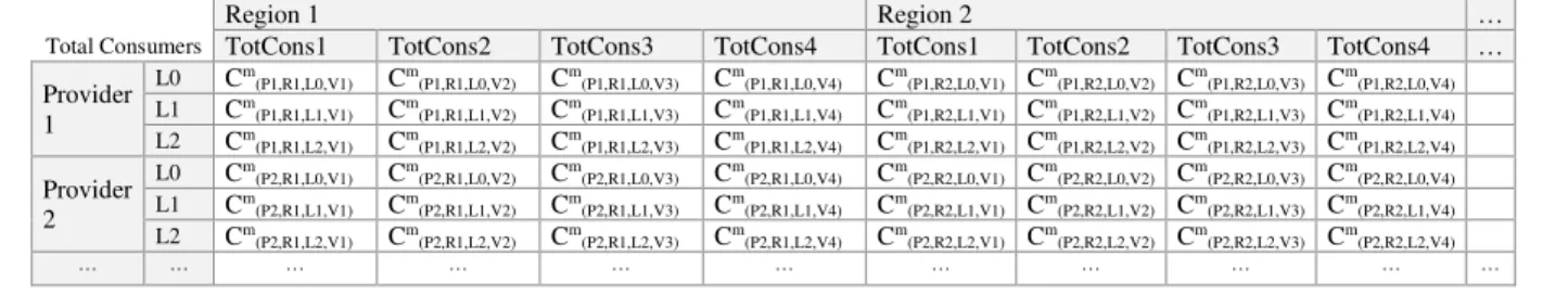
different for each provider depending of the total number of subscribers – scale economies. This means that the marginal cost can decrease when a specific provider buys higher quantities of equipment, cable, etc. (see Table 3:).

Table 3: Structure of marginal costs input parameter

Region 1 Region 2 …

Total Consumers TotCons1 TotCons2 TotCons3 TotCons4 TotCons1 TotCons2 TotCons3 TotCons4 … Provider

1

L0 Cm

(P1,R1,L0,V1) Cm(P1,R1,L0,V2) Cm(P1,R1,L0,V3) Cm(P1,R1,L0,V4) Cm(P1,R2,L0,V1) Cm(P1,R2,L0,V2) Cm(P1,R2,L0,V3) Cm(P1,R2,L0,V4) L1 Cm

(P1,R1,L2,V1) Cm(P1,R1,L2,V2) Cm(P1,R1,L2,V3) Cm(P1,R1,L2,V4) Cm(P1,R2,L2,V1) Cm(P1,R2,L2,V2) Cm(P1,R2,L2,V3) Cm(P1,R2,L2,V4)

Provider 2

L0 Cm

(P2,R1,L2,V1) Cm(P2,R1,L2,V2) Cm(P2,R1,L2,V3) Cm(P2,R1,L2,V4) Cm(P2,R2,L2,V1) Cm(P2,R2,L2,V2) Cm(P2,R2,L2,V3) Cm(P2,R2,L2,V4)

… … … …

3.2 Pricing strategy

Both suppliers and consumers aim at maximizing the benefit or surplus they receive [9]. The suppliers aim at maximizing the profit, which is the difference between revenue and cost. The consumers aim at maximizing the consumer surplus, which is the difference between consumer value (also known as utility or maximum willingness to pay) and price. As discussed, some of the factors that are important in the design of pricing scheme include technology risks, availability of resources, competition, supplier and consumer behavior, price discrimination and regulation.

3.2.1 Definition of the variation in retail prices

The definition of retail prices and trend was explained previously. For the game-theoretic tool, we need to define the variation in retail prices which we want to simulate. So, for each service, we define the price values we wish to simulate - the tool gives the possibility to simulate n values. In the example presented in the next table, the tool simulates the results obtained when the value of service 1 is Pr S1,Value1, Pr S1,Value1, Pr S1,Value1, and Pr S1,Value1 for all players (providers).

Table 4: Variation values for retail prices

Value 1 Value 2 Value 3 Value 4 … Value for Service 1 Pr S1, Value1 Pr S1, Value2 Pr S1, Value3 Pr S1, Value4 Value for Service 2 Pr S2, Value1 Pr S2, Value2 Pr S2, Value3 Pr S2, Value4 …

3.3 Definition of the variation in wholesale prices

For wholesale prices, we define the variation in wholesale price layers that we want to simulate. Similarly, for retail price, for each layer we define the price values we wish

to simulatethe tool gives the possibility to simulate n values.

(7)

Value 1 Value 2 Value 3 Value 4 … Value for Layer 0 Pw

L0, Value1 Pw L0, Value2 Pw L0, Value3 Pw L0, Value4

Value for Layer 1 Pw

L1, Value1 Pw L1, Value2 Pw L1, Value3 Pw L1, Value4

Value for Layer 2 Pw

L2, Value1 Pw L2, Value2 Pw L2 ,Value3 Pw L2, Value4

For infrastructure, the definition of which layer or combination of layers we would like to simulate is also required: conduit, cable or Bit-Stream (Conduit + Cable + Equipment).

4. Simulation model (modeling competition)

The simulation model can be sub-divided into seven main parts: retail and wholesale modeling, calculate total costs (build and lease infrastructure), calculate revenues (retail and wholesale market), calculate profit, calculate consumer surplus, and calculate welfare.

In retail modeling, we assume that consumers choose the service from the provider with the lowest price. However, consumers only buy a service if the price is less than their willingness to pay. This means that if there are two or more providers, consumers choose the service from the provider with the lowest price. Moreover, if several providers have the same price, we use the provider ranking. We also assume that consumers have a different willingness to pay for each service. First, the tool identify the retail provider for each service in the regions in study using information from providers, retail prices, consumer willingness to pay, and provider rank. Next, as we know which provider will provide each service, we can compute the total subscribers per region, service, and provider (market segment).

Figure 2: Retail market modeling

(8)

Figure 3: Wholesale market modeling

4.3 Calculate total costs (build and lease infrastructures)

The calculation of the total costs incurred by each provider is divided in two main parts: wholesale costs and build-out costs. As sees in next figure, we use the wholesale infrastructure design computed previously and the wholesale prices charged by the infrastructure owners (i.e., payments that a specific provider gives to the infrastructure owner to buy wholesale access in order to reach consumers). We assume that the network owner charges the same wholesale price to all providers.

To calculate the build-out costs, the algorithm uses the fixed and marginal costs parameters with region parameters to compute the total costs required to deploy an entire or part of an infrastructure. The total number of consumers per region and per provider is also used to add the effect of economies of scale. When a provider buys a large quantity of equipment, the probability of attaining better prices is higher.

Figure 4: Total costs calculation

4.4 Calculate revenues, profit, consumer surplus and total welfare

(9)

Figure 5: Revenues calculation

These are primarily based on the retail prices charged by providers and the total number of consumers per provider and services computed in the retail modeling. Revenues from the retail market are equal to the product of the retail price of each service and the total customers of the service.

Next, we calculate the revenues from the wholesale market. The wholesale infrastructure provides information about the number of access leased. The revenues of a provider are the sum of all payments received from other providers that use its infrastructure to reach consumers. Finally, the total revenues of a given provider are the sum of the revenues from the retail and the wholesale market. After computing the total costs and revenues in the previous algorithms, the formula we use to calculate total profit is the difference between total revenues and total profit. The total profit is also used in the identification of the Nash equilibrium strategies.

Figure 6: Profit calculation

Consumer surplus (CS) is the difference between the total amount that consumers are willing and able to pay for each service and the total amount that they actually pay (i.e., the retail price). So, the CS of a specific market is the sum of the individual consumer surpluses of all those customers in the market who actually bought the service at the going retail price [10]. To compute CS, we need information about consumer willingness to pay and retail prices for each service.

(10)

5 Results

Based on the numerous input parameters described, our tool computes several results, including profit, consumer surplus, welfare, market served, network size, costs, and revenues, and finds the strategies that are Nash equilibriums. The results are saved in text files (see Figure 7: ).

Figure 7: Structure of the results produced (output from tool)

Figure 7: show the structure of the results that correspond to a scenario of two providers, two retail services, two infrastructure layers, and two regions. Each line is a strategy. We consider a strategy to be a set of retail and wholesale prices. For each combination of prices, the tool calculates profit, CS, welfare, market served, network size, and total costs.

In addition to the results presented in the tables, the tool creates several types of graphs. Next figures show two examples of the graphs produced. The graph shows the impact on profit of both providers and variation in wholesale and retail prices. This representation gives users a tool to gain a better perspective of the results.

(11)

6 Conclusion

Sensitivity analysis shows the impact that changes in a certain parameter will have on the model’s outcome. As the interaction between all the players is important, we put the competition component in the business case. With game theory, we want to understand the effects of the interaction between the different players defined in our business case. In the proposed games, the profit (outcome) of each operator (player) will be dependent not only on their actions, but also on the actions of the other operators in the market.

The impact of the price (retail and wholesale) variations on several output results: players’ profit, consumer surplus, welfare, costs, service adoption, and so on. For that, two price-setting games are played. Players’ profits and NPV are used as the payoff for the players in the games analyzed.

In our model we also use the Nash equilibrium to find equilibrium. Proposed tools include a module to search the Nash equilibrium in the game. One strategy is a Nash equilibrium when both competitors play their best strategy related to the other strategies selected (players know each other’s strategy in advance).

References

1. Yongkang, X., S. Xiuming, and R. Yong, Game theory models for IEEE 802.11 DCF in wireless ad hoc networks. Communications Magazine, IEEE, 2005. 43(3): p. S22-S26. 2. Machado, R. and S. Tekinay, A survey of game-theoretic approaches in wireless sensor

networks. Comput. Netw., 2008. 52(16): p. 3047-3061.

3. Pereira, J.P.R., Effects of NGNs on Market Definition, in Advances in Information Systems and Technologies, Á. Rocha, et al., Editors. 2013, Springer Berlin Heidelberg. p. 939-949. 4. Verbrugge, S., et al., White paper: Practical steps in techno-economic evaluation of network

deployment planning, 2009, UGent/IBBT: Gent, Belgium. p. 45.

5. Easley, D. and J. Kleinberg, Networks, Crowds, and Markets: Reasoning About a Highly Connected World2010, Cambridge: Cambridge University Press

6. Pereira, J.P.R., Infrastructure vs. Access Competition in NGNs, in Intelligent Information and Database Systems, A. Selamat, N. Nguyen, and H. Haron, Editors. 2013, Springer Berlin Heidelberg. p. 529-538.

7. Pereira, J.P. and P. Ferreira. Next Generation Access Networks (NGANs) and the geographical segmentation of markets. in The Tenth International Conference on Networks (ICN 2011). 2011. St. Maarten, The Netherlands Antilles.

8. Amendola, G.B. and L.M. Pupillo. The Economics of Next Generation Access Networks and Regulatory Governance in Europe: One Size Does not Fit All. in 18th ITS Regional Conference. 2007. Istanbul, Turkey.

9. ITU-T, Telecom Network Planning for evolving Network Architectures, 2008, INTERNATIONAL TELECOMMUNICATION UNION. p. 208.